Application of Lateral Transshipment in Cost Reduction of Decentralized Systems

Abstract

COVID-19 has exposed the global supply chains to great vulnerability. In such extreme circumstances, product availability becomes a primary concern. This paper studies a basic inventory management strategy—lateral transshipment—under decentralized systems, which may play an important role in dealing with stockouts during unexpected crises. Lateral transshipments not only react quickly to stockout, but are also environmentally friendly due to the significant reduction of production and transportation pollution. This paper studies optimal lateral transshipment and replenishment decisions under a decentralized setting. We construct a multi-stage stochastic model that captures demand uncertainty and customer switching behavior. We demonstrate that, similar to the centralized setting, the optimal transshipment decision follows a double-threshold structure. The optimal replenishment quantities are determined under two pricing mechanisms—individual mechanism (IP) and negotiated mechanism (NP). Numerical examples are provided to demonstrate the impact of lateral transshipment on supply chain cost reduction.

1. Introduction

The outbreak of coronavirus disease 2019 (COVID-19) may change the global supply chains permanently. On one hand, some traditional businesses have been completely shut down due to containment policies and trade restrictions. For example, food security alerts arise after the lockdown of about one-third of the world’s population [1,2] and sea transport is also disrupted [3]. Even though there have been many progresses on predicting COVID-19 [4,5,6], no cure or vaccine is available now. The sustainability of global supply chains will still be under threat if demand cannot recover in a timely fashion. On the other hand, the prosperous “new retailing” has greatly helped in China’s case. Consumers make orders online from online retailers such as jd.com and Alibaba, and then pick up offline, thus avoiding unnecessary physical interactions, which helps to maintain the sustainability of the food supply chain during the pandemic. Furthermore, various online platforms are available to maintain undisrupted service and telecom companies provide free programs for amusement. To conclude, the facilitation of modern information technology, such as big data, artificial intelligence, etc., is essential for traditional companies to survive, as new technology is not only more efficient, but also more resilient under extreme circumstances.

The sharp contrast above inspires us to rethink about how to build a sustainable supply chain in case of unexpected crises in the future. In a review of sustainable supply chain management in small and medium enterprises [7,8], business, environmental and social dimensions are used, however, they are inconsistent measures in essence [9,10], which needs subtle balance to achieve maximum social welfare. In a systematic review of sustainable supply chain management in global supply chains [11,12], different configurations and governance modes are refined, but some unexpected shocks, such as trade friction and pandemic, are not considered. This is also the challenge facing strategic supply chain management, as in [13,14].

In our opinion, during the pandemic, the smooth flow of materials should be the first priority. As stockout is a common phenomenon that not only reduces retailers’ profits, but also damages products’ brand images, the sustainability of the whole supply chain, and even the lives of healthcare workers and ordinary people around the world. That is one main reason that we pay more attention to basic inventory management at the present time, despite it being a very traditional measure to maintain supply chain sustainability. Besides that, good inventory management helps to reduce not only transportation cost, but also procurement cost, due to more accurate demand and supply coordination. From the perspective of sustainable procurement or green public procurement [15], cost reduction by inventory management helps address a key issue of financial constraint in practice, as discussed by Brammer and Walker [16]. There have been a substantial number of studies about inventory management, of which one stream is lateral transshipment. Lateral transshipments within an inventory system are stock movements between locations of the same echelon. With improved tracking accuracy, lateral transshipment between different stores gains its popularity, because every store can also function as a warehouse to meet the customers’ needs, in case of shortage at other stores.

Nowadays, it is common to see lateral transshipments between different stores. The reasons may be that (1) it is faster to respond to consumers compared to emergency orders, (2) it saves energy from unnecessary production, especially for perishable goods, and (3) it reduces the potential pollution, due to long-distance transportation from the central warehouse. In this paper we study the optimal transshipment decisions and inventory replenishment decisions under a decentralized setting. We review some related literature on lateral transshipment in the next section.

2. Literature Review

There have been plenty of studies on lateral transshipment, and Paterson et al. [17] provide a thorough literature review. Huang [18] presents a comprehensive review on supply chain relationships in the presence of transshipment. According to Paterson et al. [17], the research is categorized into two streams: proactive and reactive. Proactive lateral transshipment distributes inventory among stores or warehouses before the realization of demand, while reactive lateral transshipment distributes left-over inventory among stores or warehouses after the realization of demand. We plot the structure of different streams in Figure 1.

This paper falls into the category of decentralized systems. In this category, Rudi et al. [19] provide one of the first studies on lateral transshipment in a decentralized system and lay a basic study frame with game theory. They show the uniqueness of Nash equilibrium in order quantities for two retailers. Later, different decision mechanisms are developed. Anupindi et al. [20], Granot and Sosic [21], and Sosic [22] study cooperative games at the transshipment stage and non-cooperative games at other stages. Rong et al. [23] analyze preventive transshipments before realization information can be fully observed and show a dominant transfer policy. Zhao et al. [24] examine e-commercial supply chain performances, with or without a lateral transshipment option. Yan and Zhao [25] study information asymmetry issues between a manufacturer and two retailers, where lateral transshipment can be used as a way of inventory sharing.

In the centralized category, Krishnan and Rao [26] are the first to consider lateral transshipment within the same echelon after demand realization. Plenty of variations and extensions have been built upon Krishnan and Rao’s model. Robinson [27] studies a multi-location, multi-period problem, and finds the optimal solutions for multiple identical locations or two non-identical locations. Herer and Rashit [28] examine a two-location inventory system, considering both fixed transshipment costs and a joint replenishment cost. Wee and Dada [29] analyze transshipment policies under different assumptions related to coordination of retailer inventory and warehouse inventory. Hu et al. [30] study the lateral transshipment quantity, from the perspective of both demand uncertainty and capacity uncertainty. Zhao et al. [31] analyze the optimal production and transshipment policy for a two-location, make-to-stock queuing system.

Among the existing literature on lateral transshipment within decentralized supply chains, the model proposed by Li et al. [32] is the closest to ours. Motivated by Best Buy’s new operations strategy that asks its brick-and-mortar stores to do double duty as warehouses, Li et al. [32] investigated a retailer’s optimal transshipment and replenishment decisions at two nearby local stores. Li et al. [32] considered a single-period, two-store model where transshipment and replenishment costs are both accounted for. More importantly, different from traditional automatic request from stores in shortage, and automatic respondence from stores with excess stock, Li et al. [32] introduced the partial request and random switching to describe two common consumer behaviors.

There are also many models considering switching with various switching rules. In the model of Lippman and McCardle [33], the switching rules of initial and remaining demand are endogenous, while Anupindi and Bassok [34] use a deterministic exogenous switch rate to study a system with one manufacturer and N retailers. However, those two papers do not allow transshipments. In the paper of Zhao and Atkins [35], they consider transshipment and switching as “market-driven” and “customer driven”, which are mutually exclusive alternatives to retailers. Jiang and Anupindi [36] combine the preferences of the manufacturer, the retailers, and the customers, to explore the impact of the search methods and the transfer price scheme on safety stock and retail prices. Comez et al. [37] study the transshipment dynamics between competing retailers, in a continuous-time model. As found in the study of Li et al. [32], besides complete sharing and no sharing, there are feasible solutions lying in between, due to uncertainty of consumer behavior. Liao et al. [38] compare the performances of emergency orders, lateral transshipment and a hybrid of them. Partial request and switching are both allowed. However, the switch rate is a constant in the model proposed by Liao et al. [38].

Different from the existing literature, Li et al. [32] use partial request, instead of automatic request from the stockout store. This happens when the revenue from transshipment is fully countervailed by transshipment price and transportation cost, thus, the shortage store may request a proportion of the gap. Random switching is used to illustrate the uncertainty of consumer behavior when faced with stockout. The unmet demands may turn to the competing stores, and the surplus stores will deny the request for transshipment in favor of forthcoming consumers. As switching behavior is personal and may be spontaneous, random switching setting will be more reasonable than fixed exogenous rate. Li et al. [32] show that the optimal transshipment policy follows a double-threshold structure when the prospect of the switched demand is not large enough; and a transshipment quantity of zero becomes optimal otherwise.

Our model differs from Li et al. [32], in that this paper optimizes transshipment and replenishment under decentralized systems, instead of centralized systems. To the best of our knowledge, this is the first transshipment paper to introduce random variables to investigate the uncertain customer switching behaviors under a decentralized setting. We try to fill this gap because, even though the majority of lateral transshipment literature constructs models in a centralized system, there are many situations where complete inventory pooling is impossible, for example, the case of auto parts in the study of Rudi et al. [19] In a survey of 71,000 customers, Corsten and Gruen [39] find that customers lose patience with stockouts. That is the situation where a decentralized system works out by meeting the customers’ need in a timely manner. The COVID-19 pandemic further reinforces the necessity, because emergency orders cannot be filled due to massive lockdowns.

The remainder of this paper is organized as follows. We describe our methodology that allows both partial request and random switching in Section 3 and derive the optimal transshipment and replenishment quantities. Later, results from numerical experiments are thoroughly discussed and compared with extant literature in Section 4. We conclude the paper in Section 5. All the proofs are presented in Appendix A.

3. Methodology

3.1. Basic Model Settings

This paper considers two local markets, with two stores $i$ and $j$($i$, $j$$\in${1,2}) selling the same products. We focus on a perishable product and hence a single period. We use $D_i$ to represent the independent, stochastic, local demand faced by Store $i$, for $i=1,2$. Furthermore, $G_i(d_i)$ and $g_i(d_i)$ are used to represent the cumulative distribution function (cdf) and the probability density function (pdf) of local demand $D_i$, respectively.

The typical events flows are as follows.

• First, each store determines the replenishment level. $Q_i$ and $Q_j$ before realization of demand.
• Second, the local demands are realized respectively, with the realization of $d_i$ and $d_j$, without loss of generality, say Store $i$ has excess stock, while Store $j$ runs out of stock, i.e., $Q_i>d_i$ and $Q_j<d_j$.
• Third, Store $j$ requests transshipment from Store $i$.
• Fourth, surplus Store $i$ determines the transshipment quantity $q_{ij}$ to be shipped to Store $j$ before the observation of potential demand from unmet customers.
• Fifth, unsatisfied customers of Store $j$ switch to Store $i$.
• Sixth, both stores collect revenue.

When demand realizations are observed in the second stage, the unmet customer has three choices: wait at Store $j$ for replenishment, switch to nearby Store $i$, and give up buying. This is the source of differentiated switching customers, which will be discussed further.

When it comes to requests for transshipment, we refer to ${\psi }_j\in [0,1]$ as Store $j$’s “request rate”, which represents the percentage of the initially unmet demand at Store $j$. In this paper, we assume that ${\psi }_j$ is a known constant for the retailer and the amount of the transshipment demand can be obtained by ${\psi }_j\left(d_j-Q_j\right)$.

Upon receiving the transshipment request, Store $i$ must determine $q_{ij}$: the transshipment quantity from Store $i$ to Store $j$. The upper bound on $q_{ij}$ is determined by the two stores’ abundance and shortage levels. Firstly, $q_{ij}$ cannot exceed Store $i$’s surplus $Q_i-d_i$. Secondly, $q_{ij}$ cannot exceed the requested demand: ${\psi }_j(d_j-Q_j)$. So, $0\le q_{ij}\le {\overline{q}}_{ij}\equiv min{\{\mathrm{Q}}_i-d_i,{\psi }_j(d_j-Q_j)\}$. It is worth noting that Store $j$ will face another uncertain demand because, while the transshipment request is addressed at this point, customer switching demand is not observed yet. Store $i$ has to balance between unseen future opportunities and the current chance to reduce the leftover inventory. This sequence of events creates another reason for the surplus store to partially fulfill the transshipment demand: reserving inventory for the switched demand flowing to Store $i$.

The transshipment stage is then followed by the switching stage. Moreover, ${\Omega }_j$ is used as Store $j$’s “switch rate”, and ${\omega }_j$ is the realization of ${\Omega }_j$, which represents the percentage of the ultimately unmet demand at Store $j$ that is switched to Store $i$. We assume that ${\Omega }_j$ is a random variable within $[0,1]$, and $F_j({\omega }_j)$, $f_j({\omega }_j)$ are referred to as the cdf and pdf of ${\Omega }_j$ respectively. Note that the amount of the ultimately unmet demand at Store $j$ is $d_j-Q_j-q_{ij}$. The amount of the switched demand is, therefore, ${\Omega }_j(d_j-Q_j-q_{ij})$. It is worth comparing the initially unmet demand with ultimately unmet demand. As initially unmet demand can be split into three streams, the ultimately unmet demand can also be divided into two streams: the initially unmet demand and rejected transshipment demand.

In a centralized system, the entire company incurs all the costs and collects all the revenue, while in a decentralized system, the stores make their own decisions in order to maximize their individual profits, with each bearing their own costs and colleting their own revenue. When the surplus store sends a transshipment to the shortage store, we assume the surplus store bears the cost of transshipment and the shortage store pays a price for each unit of transshipment, as in the study of Rudi et al. [19]. We use $p_{ij}$ to denote the price Store $j$ pays Store $i$ for each unit of transshipment and assume that $r_j>p_{ij}>{\tau }_{ij}+s_i$. We consider two different mechanisms for choosing transshipment prices. One is the individual price (IP) mechanism, where transshipment prices are determined by the stores individually in advance, and the other is the negotiated price (NP) mechanism where the two stores negotiate a pair of $(p_{ij},p_{ji})$. Before observing their local demand, the two stores independently set their replenishment levels. After the transshipment quantity is decided, the shortage store pays the surplus store $p_{ij}$ per unit for transshipment, but the unit transshipment cost is paid by the surplus store.

In addition to event descriptions, some necessary monetary parameters are introduced, as listed in

Table 1. Summary of Main Notations.

Decision Variables
$Q_i$	replenishment inventory level at Store $i$;
$q_{ij}$	transshipment quantity from Store $i$ to Store $j$;
Model Parameters
$c_i$	unit procurement at Store $i$;
$r_i$	unit revenue at Store $i$ in local markets;
$s_i$	unit salvage value at Store $i$;
${\tau }_{ij}$	unit transshipment cost from Store $i$ to Store $j$;
$p_{ij}$	unit revenue at Store $i$ for transshipment;
${\psi }_i$	request rate at Store $i$;
$D_i$	local demand with a realization of $d_i$, a cdf of $G_i$ and a pdf of $g_i$
${\Omega }_i$	switch rate at Store $i$ percentage of Store $i$’s ultimately unmet demand that is switched to Store $j$ with a realization of ${\omega }_i$, a cdf of $F_i({\omega }_i)$ and a pdf of $f_i({\omega }_i)$;

. For $i,j\in \left\{1,2\right\}$ and $j\ne i$ the cost of procuring one unit of inventory is $c_i$ at Store $i$; each unit sold by Store $i$ brings in a revenue of $r_i$ when it is sold to either local demand or switched demand; ${\tau }_{ij}$ is transshipping cost for each unit inventory from Store $i$ to Store $j$, and is incurred by the seller, i.e., Store $i$; the salvage value at Store $i$ at the end of the period $s_i$; loss of good will cost for the unmet demand is assumed to be zero.

To avoid trivial optimal decisions, we make a few assumptions as Rudi et al. [19] For $i,j\in \left\{1,2\right\}$ and $j\ne i$, the following assumptions hold throughout the paper.

• $c_i<r_i$;
• $s_i<p_{ij}-{\tau }_{ij}<r_j-{\tau }_{ij}$;
• $r_j-r_i<{\tau }_{ij},s_j-s_i<{\tau }_{ij},c_j-c_i<{\tau }_{ij}$;
• $p_{ij}\le r_j$

The first two inequalities guarantee the seller’s profit, and the third group of inequalities prohibit one from arbitraging. When $p_{ij}=r_j$ holds in the fourth inequality, the systems can be considered as centralized, as unit transshipment quantity from the surplus store collects all the unit revenue from the shortage store.

Further, as there are four random variables in our model: $D_i,D_j,{\Omega }_i,{\Omega }_j$, in the interest of tractability, we assume that their distributions $G_i$’s and $F_i$’s are twice differentiable and strictly increasing throughout the paper.

3.2. Optimal Transshipment Quantity

In the centralized systems, the decision maker, naturally, observes demand realizations at both stores. When the stores are each on their own, the demand realization and replenishment level at an individual store may be the store’s private information. Our approach is to assume that the shortage amount and the surplus amount are public information. This assumption helps with trackability, while granting the stores a level of privacy.

Without loss of generality, we let Store $i$ be the surplus store and Store $j$ the shortage store when deriving the optimal transshipment policy. Denote by ${\pi }^d$ Store $i$’s optimal, conditional profit when $d_i<Q_i$ and $d_j>Q_j$. Store $i$ pays $c_i{Q}_i$ to replenish its inventory, earns a revenue of $r_i{d}_i$ from satisfying local demand, a margin of $(p_{ij}-{\tau }_{ij})q_{ij}$ from transshipment, an expected revenue of $r_i{E}_{{\Omega }_j}min(L_i,{\Omega }_j{L}_j)$, where $L_i\equiv Q_i-d_i-q_{ij}$ representing the inventory level prepared for the forthcoming switching demand, and $L_j\equiv d_j-Q_j-q_{ij}$ representing the ultimate unmet demand from shortage store, an expected salvage value of $s_i{E}_{{\Omega }_j}max(L_i-{\Omega }_j{L}_j,0)$ from eventual leftovers. Apparently, Store $i$ would like to choose $q_{ij}\le {\overline{q}}_{ij}\equiv min(Q_i-d_i,{\psi }_j(d_j-Q_j))$ wisely, so that $q_{ij}$ results in ${\pi }^d$. Putting together those elements, we have

$$\begin{array}{c}{\pi }_i^d(Q_i,d_i,Q_j,d_j|d_i-Q_i<0,d_j-Q_j>0)\\ =r_i{d}_i-c_i{Q}_i+ma{x}_{q_{ij}<{\overline{q}}_{ij}}\{(p_{ij}-{\tau }_{ij})q_{ij}\\ +r_i{E}_{{\Omega }_j}min(L_i,{\Omega }_j{L}_j)\\ +s_i{E}_{{\Omega }_j}max(L_i-{\Omega }_j{L}_j,0)\}\end{array}$$

With $q_{ij}^d$ representing Store i’s optimal transshipment quantity in the decentralized setting, we formalize our results in Proposition 1.

Proposition 1.

Suppose$d_i<Q_i$and$d_j>Q_j,Z_i=\frac{Q_i-d_i}{d_j-Q_j}$, the optimal transshipment policy is as follows.

(1) 

If$p_{ij}\le {\tau }_{ij}+s_i+(r_i-s_i)E{\Omega }_j$, then$q_{ij}^d\equiv 0$.

(2) 

Otherwise, there are two thresholds:$z_i^d$and${\overline{z}}_i^d$such that$z_i^d<{\overline{z}}_i^d=(1-z_i^d){\psi }_j+z_i^d$, and${\displaystyle {\int }_0^{z_i^d}(1-{\omega }_j)d{F}_j({\omega }_j)\le \frac{r_i-p_{ij}+{\tau }_{ij}}{r_i-s_i}}$. The optimal transshipment quantity is determined based how$Z_i=\frac{Q_i-d_i}{d_j-Q_j}$compares to the two thresholds. Specifically, (2a) if$Z_i\ge {\overline{z}}_i^d$, we have$q_{ij}^d={\psi }_j(d_j-Q_j)$; (2b)${\overline{z}}_i^d\ge Z_i\ge z_i^d\Rightarrow q_{ij}^d=\frac{Q_i-d_i-z_i^d(d_j-Q_j)}{1-z_i^d}$; and (2c) if$Z_i\le z_i^d\Rightarrow q_{ij}^d=0$.

Proposition 1 indicates that the optimal transshipment policy in the decentralized setting follows the structure of the optimal transshipment policy in the centralized setting. The main difference lies in the thresholds. Newsvendor-like critical ratios are applied in both policies to characterize the thresholds, while $r_j$ is used in the centralized setting for the calculation of its critical ratio. The transshipment price $p_{ij}$ is used in the decentralized setting. This makes sense because the transshipment quantity $q_{ij}$ is determined by Store $i$ in the decentralized setting, and Store $i$ cares more about $p_{ij}$ (i.e., what Store $i$ earns for each unit of transshipment sent) than about $r_j$ (i.e., what Store $j$ earns for each unit of transshipment received). Building upon this insight, we establish Corollary 1.

Corollary 1.

For any given set of$\left(Q_i,Q_j,d_i,d_j\right)$,$q_{ij}^d\le q_{ij}^c$and$q_{ij}^c-q_{ij}^d$decreases in$p_{ij}$. If$p_{ij}=r_j$, then$q_{ij}^d=q_{ij}^c$. Where$q_{ij}^c$is the optimal transshipment under centralized system.

Corollary 1 suggests that, when the surplus store gets to decide, on its own, the transshipment quantity, its transshipment price matters. The higher the price $p_{ij}$, the more attractive transshipment is to Store $i$ and the higher the optimal transshipment quantity $q_{ij}^c=q_{ij}^d$. Since Store $i$ cannot charge a transshipment price $p_{ij}$ that is higher than $r_j$ (i.e., Store j’s revenue from selling a unit), the optimal transshipment quantity in the centralized setting sets an upper bound on the optimal transshipment quantity in the decentralized setting. In contrast, Rudi et al. [19] find that it is optimal for the surplus store to transship all surplus inventory to the shortage store, if necessary, and refer to the policy as “complete pooling”. Moreover, in the model studied by Rudi et al. [19], the surplus store’s optimal transshipment quantity is independent of its transshipment price or whether the setting is centralized or decentralized.

Rong et al. [23] also derive an optimal double-threshold transshipment policy, which is referred to as the “Control-Band Conserving” (CBC) policy. However, the CBC policy applies in a multi-period setting, where demand is partially observed in the first subperiod and fully revealed in the second subperiod. Under the CBC policy, control bands are established using inventory positions. Store $i$ compares its inventory position $I_i$ with respect to two thresholds $I_i^L$ and $I_i^H$. It requests to ship in $I_i^L-I_i$ if $I_i<I_i^L$, to ship out $I_i-I_i^H$ if $I_i>I_i^H$, and nothing if $I_i^H>I_i>I_i^L$. As a result, if both stores request to ship in or if both of them want to ship out, no transshipment is made; otherwise, the transshipped quantity is equal to the minimum of the requested shipping-in and shipping-out amounts. Transshipments are used strategically to prevent future shortages in Rong et al. [23] In contrast, our double-threshold policy applies in a single-period setting with responsive transshipment, and the optimal transshipment quantity depends not on inventory positions, but on the surplus-shortage-ratio. Our model reveals an incentive in a single-period setting for strategic transshipment decision: reserving inventory for the switched demand.

3.3. Optimal Replenishment Quantity

The derivation of the surplus store’s optimal transshipment quantity allows us to further explore the store’s replenishment decisions. When running independently, the two stores determine their own replenishment levels independently and privately. However, each store’s ultimate profit depends on the other’s replenishment level. Let ${\pi }_i^d(Q_i,Q_j,p_{ij},p_{ji})$ represent Store $i$’s expected profit given a pair of replenishment levels and a pair of transshipment prices. Note here that, while Store $i$ observes its own replenishment level and both transshipment prices, Store $j$’s replenishment level remains unknown to Store $i$. To find a sensible solution, we look for equilibrium replenishment levels: $y_i^d$ and $y_j^d$. Theorem 1 characterizes the independent stores’ equilibrium replenishment levels under the individual price (IP) mechanism and the negotiated price (NP) mechanism, respectively.

Theorem 1.

(a) Under the individual Price mechanism, the equilibrium transshipment prices are$({\overline{p}}_{12},{\overline{p}}_{21})=(r_2,r_1)$, and the equilibrium replenishment levels$({\overline{y}}_1^d,{\overline{y}}_2^d)$can be uniquely determined with$y_1^d+y_2^d>y_1^c+y_2^c$. (b) Under the Negotiated Price mechanism, the equilibrium replenishment levels$(y_1^d,y_2^d)$corresponding to$(p_{12},p_{21})$have the following properties: (1) if$g_1(g)$and$g_2(g)$are non-increasing functions$(y_1^d,y_2^d)$is unique; (2)$y_1^d+y_2^d$increases in$p_{ij}$; (3)${\pi }_1^d(y_1^d,y_2^d)+{\pi }_2^d(y_1^d,y_2^d)<{\pi }^c(y_1^c,y_2^c)$.

Under the IP mechanism, the equilibrium transshipment price charged by the surplus store is the same as the unit revenue at the shortage store. Consequently, the fulfilled transshipment does not bring in any additional gain for the shortage store. This makes the stores more inclined to avoid shortage, and hence results in higher replenishment levels at equilibrium in the decentralized setting than in the centralized setting. Under the NP mechanism, we are able to show that the sum of the equilibrium replenishment levels increases in the transshipment price. However, it is unclear how the sum of the equilibrium replenishment levels compares to the sum of the optimal replenishment levels in the centralized setting. The challenges are similar to those documented in Hu et al. [40]

4. Results and Discussion

Theoretically, centralized systems work better than decentralized systems, given rigid assumptions, one of which is the perfect coordination between stores. In this paper, we demonstrate that lateral transshipment also works well in saving the total cost of the supply chain in decentralized systems. As a result, we focus on the total supply chain cost reduction, even though there is no coordination from a virtual principal or parent company. To achieve this goal, we provide two benchmarks where the stores make independent decisions. The first one is the total cost from the two independent stores without transshipment and each adopting newsvendor model. The second one is the total cost from the two independent stores while fully satisfying transshipment requests from shortage stores. It captures the complete pooling scenario with full cooperation.

To make meaningful comparisons, we compute the optimal inventory levels and profits under three scenarios. The first two focus on individual profit, while the third maximizes the total supply profits. Numerical results demonstrate perfect symmetry, that is, when Store 1 aims to maximize its own profit, it will replenish the maximum possible stock within the given upper bound, while Store 2 replenishes the lower bound, and vice versa. This makes sense, given the settings of decentralized systems with random switching and partial request, because each of the two stores strives to obtain the entire profit from the supply chain.

In order to measure the total cost saved by the lateral transshipment decisions, we compute the proportion of total profit from our model to those of the aforementioned benchmarks, given that total profit is the opposite of total cost and total cost is negative. The comparisons are made between our model against newsvendor models and full transshipment models without random switching, denoted by $I2N$, $I2F$ respectively, corresponding to the first two scenarios, and $T2N$, $T2F$ respectively corresponding to the third scenario. We normalize the benchmark cases to 100%, therefore more than 100% indicates an increase and improvement, while less than 100% indicates a decrease and suboptimal situation. For inventory comparisons, the same mechanisms hold, except that a number greater than 100% indicates suboptimality due to increased carrying cost. The other monetary parameters used in our experiment are described below, and special treatments are applied to avoid trivial situations.

We assume a uniformly distributed local demand of $[0,200]$ for both stores, and symmetric monetary parameters with $r_1=r_2=100$, $p_{12}=p_{21}=95$, ${\tau }_{12}={\tau }_{21}=80$, $c_1=c_2=10$, $s_1=s_2=3$. Partial request rate ${\psi }_i$ starts from 0.1 with a step length of 0.1 to 1, for $i=1,2$. The random switch rate ${\Omega }_i$ complies to uniform distribution, belonging to $\{(0,0.1),(0,0.2),(0,0.3),(0,0.4),(0,0.5),(0,0.6)\}$. In Section 4.1 and Section 4.2, this paper first investigates the situations where the two stores hold the same request rates and switching rates, and then all the request rate pairs and switching rate pairs are studied.

4.1. Benchmarks

As decisions are made independently, when there are no transshipments between the stores, the optimal transshipment quantity for benchmark 1 is zero, and the optimal replenishment quantity is $(Q_1^{Bench1},Q_2^{Bench1})=(185.57,185.57)$, the maximum profit is 14,037.18.

For benchmark 2 of full transshipment, we set ${\psi }_i={\psi }_j=1$, which means that, whenever there is a shortage after the observation of local demand, the store will request full transshipment from the surplus store and the surplus store will cover the transshipment as soon as possible, which is also termed as “complete pooling”, as described in Paterson et al. [15] When each store aims to maximize its own profit, the optimal replenishment quantity is $(Q_1^{Bench2},Q_2^{Bench2})=(200,34)$ or $(34,200)$, with a maximum profit of 21,194.73 for the whole supply chain. Full lateral transshipments result in about 50.99% more profit, with less inventory. Furthermore, 29,739 out of the 40,000 pairs of combinations are found to perform better than $(Q_1^{Bench1},Q_2^{Bench1})=(185.57,185.57)$ do.

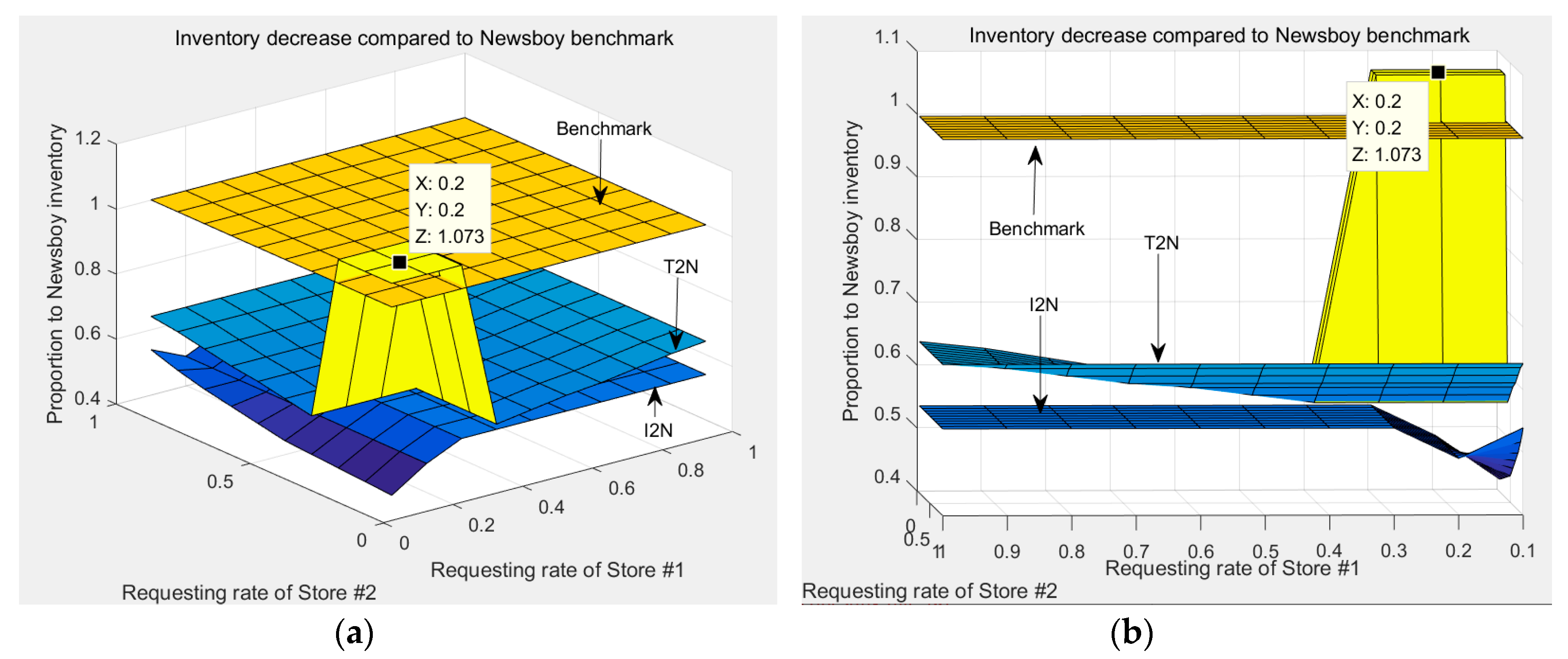
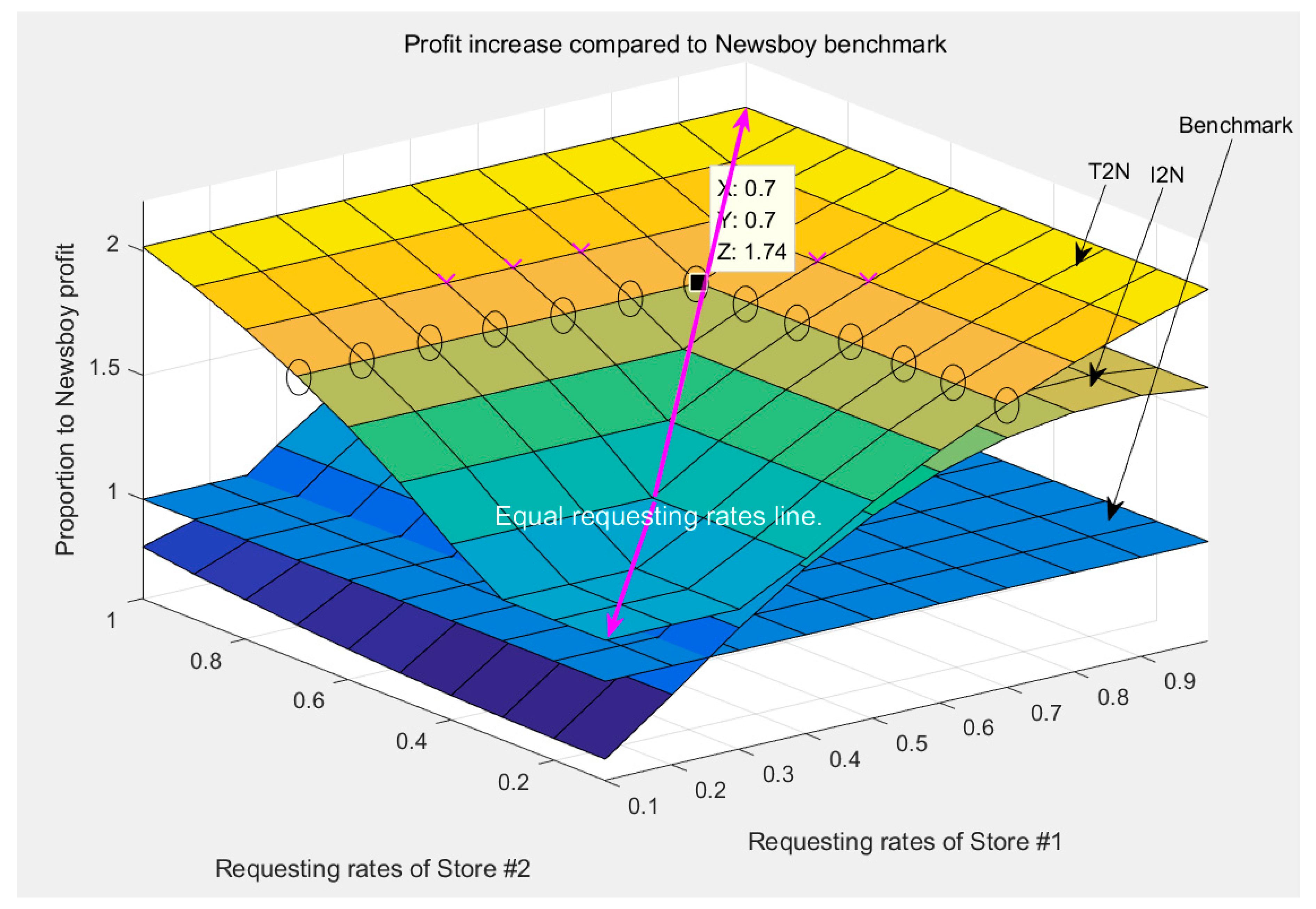
4.2. Impact of Request Rate

Figure 2 compares the performances of our model when the two stores face the same request rates. Figure 3 and Figure 4 compare the performances of our model when the two stores face different request rates, where 100 pairs are carefully examined.

From panel (a) in Figure 2, we can see that improvement is observed for all the request rates, where the total profit in the green lines corresponds to the third scenario, and is also observed in 8 out of 10 individual cases in the orange lines. With no transshipment when adopting the newsvendor model, there is little coordination of the supply chain. There is significant improvement in total cost with the increase of request rate. Given this, the request rate could be used as an indicator of the levels of coordination. However, in panel (b), only when request rates are greater than 0.6 can we conclude that our model outperforms the full transshipment model. Similar conclusions are found when the two stores hold different request rates, as in Figure 3 and Figure 4.

When facing different request rates, there are 100 combinations in our model, as shown in the 3D plot, and the benchmark is expanded into a plane with a constant value of 1. Perfect symmetry can also be found in Figure 3 panel (a). By rotating Figure 3 panel (a), we have a side view, from where the quantitative relationships are clear. Similar conclusions can be found in Figure 4. One possible explanation is that full transshipment represents close cooperation of the two stores and lower request rates in our model cannot match that advantage. However, by incorporating the random switching mechanism of the customer, our model surpasses the full transshipment as request rate increases. Furthermore, the optimal inventory levels in Figure 5, Figure 6 and Figure 7 verify our conclusion.

In panel (a) of Figure 5, individual maximization holds the lowest levels of inventory for the majority of the cases, however, it is an extreme case when the two stores stay at the two ends of the demand distribution. With our model, we observe that improvement occurs for all the request rates. Although the total inventory levels are greater than that of newsvendor for the lower request rate, the quantity decreases quickly to less than 60 percent of the benchmark when request rates are greater than 0.4, which implies significant decrease in inventory levels. Similar findings in panel (b) further confirm the judgement that lateral transshipment with partial request and random switching in decentralized systems outperform the newsvendor model and full transshipment model.

Besides that, the most interesting finding is shown in Figure 8, a revamp of Figure 3 panel (a) for the ease of understanding. The pink arrow connects all the combinations where the two stores hold the same request rate. It is clear that the maximum profit is determined only by the larger request rate, caeteris paribus. For example, the maximum profits for the combinations of $(0.7,{\psi }_2)$, ${\psi }_2\le 0.7$ and $({\psi }_1,0.7)$, ${\psi }_1\le 0.7$ are the same, i.e., 74% increase as circled by the ovals in Figure 8. If request rates can be used to measure the cooperation level, then the result implies that, provided that one party is willing to cooperate, the total value of the supply chain can be improved, and the improvement is determined by the requesting level. The logic is similar to the global trades between different countries, where rejecting international cooperation by imposing a heavy tariff does not help to improve the total welfare.

However, cooperation should be bilateral for long-term relationship development and unilateral benefit or loss will be temporary in the game between the counterparties. A similar analysis can be conducted in Figure 4 panel (a). In the next subsection, we study the relationships between optimal inventory levels and switching rates, as done in Section 4.2.

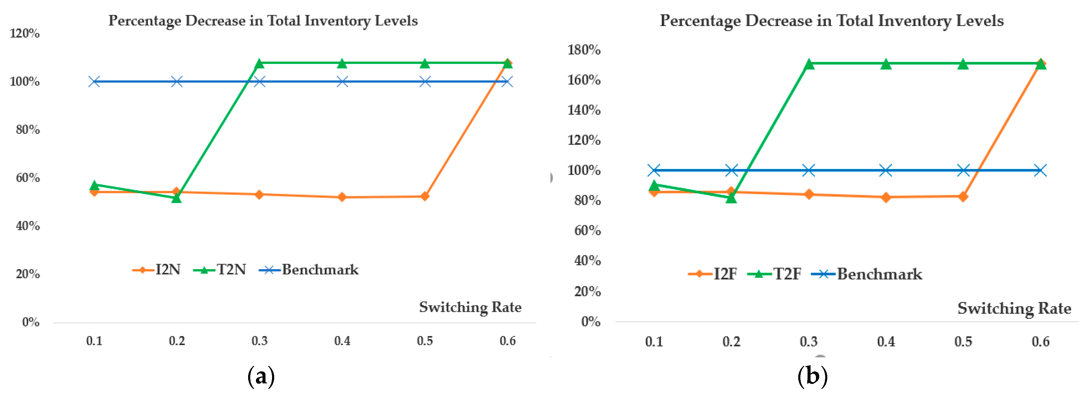
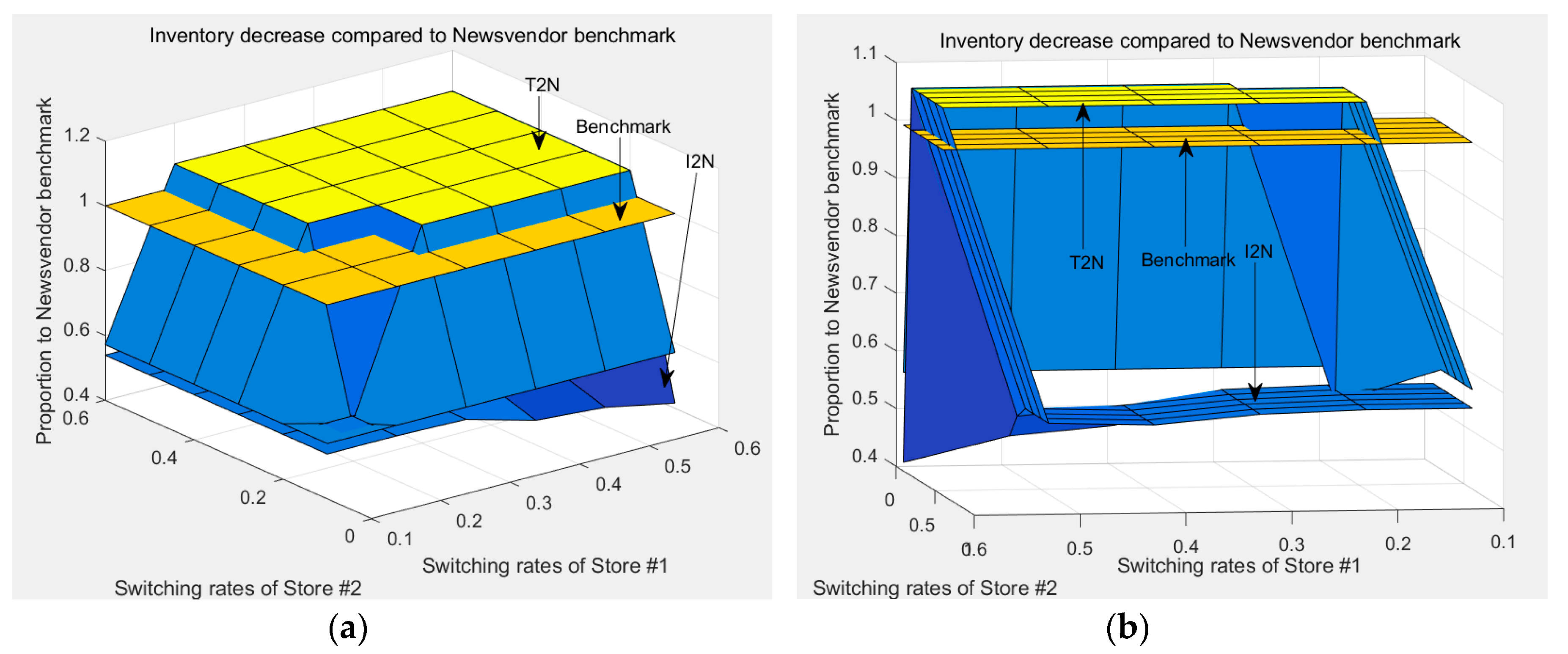
4.3. Impact of Random Switching Rate

Figure 9 compares the performances of our model when the two stores face the same switching rates. Figure 10 and Figure 11 compare the performances of our model when two stores face different switching rates, where 36 pairs are carefully examined.

The conclusions here are very different from those of Section 4.2. From Figure 9 panel (a) and (b), it can be observed that, with switching rate increasing, individual store profit declines significantly, while the total profit stays stable. In panel (a), the total profits are greater than the benchmark values, while in panel (b), the profits are lower than the benchmark values. The results from asymmetric combinations confirm the finding, as can be seen in Figure 10; Figure 11.

Figure 12, Figure 13 and Figure 14 show that total inventory levels rise quickly above the benchmark, indicating increasing carrying costs. Even though we optimize the total profit, the figures show that the maximum profits and total inventory levels decline when switching rates increase, as the cooperation from request rates is countervailed. In the proactive model developed by Zhao and Atkins [29], they consider transshipment and switching as “market-driven” and “customer driven”, which are mutually exclusive alternatives to retailers.

As a possible explanation, we conjecture that the phenomenon may be attributed to the competing mechanism. When there is a higher probability that non-local customers will switch, the stores will replenish more than they need to meet the switched demand. If there is no coordination mechanism between the competing stores, each of them will replenish much more than needed, resulting in suboptimality for the supply chain. Although this paper constructs the model under decentralized systems with reactive transshipment, the findings that switching rate may become detrimental to the retailers and to the supply chain might be worth noting when designing a sustainable supply chain.

As shown in Figure 15, this paper investigates the impact of asymmetric switching rates. There is perfect symmetry around the equal switching rate line, connected by the pink double-arrow line. However, the maximum profits are determined by the lower switching rate, which means switching rate acts against request rate. In Li et al. [32]’s centralized model, the profitability has positive relationships with both request rate and switching rate. To some extent, we may take both parameters as indicators of liquidity of materials and money, and higher values indicate better liquidity. The two indicators function the same way to increase or decrease the value of the supply chain under centralized setting, while in our model, the two indicators work against each other.

4.4. Managerial Insights

It is not always good to have tools reinforcing each other in the presence of uncertainty of business environment. When positive about the future, the manager can increase the investment and vice versa. Countervailing indicators act as hedges to each other, which will help us survive hard times, such as the long-lasting period of the COVID-19 pandemic. The result provides great help for retailers to take proper action. Practically, when faced with the increasing loss of customers and increasing request rates from competitors, the managers often turn down the request. However, the model suggests that a higher request rate will hedge the higher switching rate. The managers should not only accept the request, but also strengthen the virtual “export”. On one hand, the “export” will lead to temporary net revenues; on the other hand, customers may switch back when stuck in long lines waiting for replenishment from competing retailers.

Completely decentralized systems may be rare in an organized entity, but the situations are very common for retailers serving different brands. Our model is developed under the simplest form, but in reality, there may be many competing retailers selling more than one commodity at the same time. Besides materials and cash flows, information has been playing more and more important roles. For example, if the retailer has advanced information on customer switching rate in our model, optimization could be done in advance to maximize the profit.

5. Conclusions

5.1. Concluding Remarks

As growing attention is paid to environmental and social sustainability, the traditional definition of sustainability has been changed. However, the unexpected COVID-19 pandemic has struck the global supply chains dramatically, causing great damage to tens of thousands of lives, due to the lack of medical protections or the shortage of food. Globalization has united the world to be a centralized system, which has greatly advanced with close cooperation. However, COVID-19 exposes the global supply chain to great vulnerability and teach us a lesson to keep a certain level of independence. Inspired by both practice and Li et al. [32], this paper studies the lateral transshipment and replenishment decisions under decentralized system, where the two stores make independent decisions. The setting is common in practice, as centralized systems do not always work well, due to implicit costs from coordination failure, systems efficiency, and the sustainability of the supply chain. Decentralized systems may be inferior to centralized systems theoretically, but may perform better under extreme circumstances because of the intrinsic hedging function, specifically, countervailing effects in maximizing the profit in our model. This paper derives the unique and optimal transshipment quantities and calculates the maximum profit, assuming uniform distribution for the random variables. Numerical experiments demonstrate the positive relationship between optimal profit and request rate, and the negative relationship between optimal profit and switching rate. Contrary to the intuitive belief that retailers should turn down the request from competitors, the result promotes encouraging close cooperation, i.e., higher request rate to increase the added value to the supply chain.

5.2. Theoretical Contributions

To the best of our knowledge, most decentralized lateral transshipment models assume fixed request rates and switching rates. This paper studies optimal decisions given the uncertainty of customer behavior. The theoretical contributions are as two-fold: (1) this paper introduces random variables to study customer behavior, closing a gap in decentralized lateral transshipment literature. (2) This paper studies the impact of request rate and switching rate, providing practical suggestions to managers.

5.3. Research Limitations and Future Directions

When combined with random variables, the derivation of analytical solutions becomes far more complicated. This paper investigates a supply chain with only two nodes and one product, which is very simple compared to practice. This paper can be further extended in several aspects. To better simulate practice, we intend to increase the number of decision makers, and take strategic customers into consideration. As new retailing format and omnichannel retailing become popular, the shopping mode also changes. Future extensions can also combine omnichannel with online shopping.

References

1. Galanakis, C.M. The Food Systems in the Era of the Coronavirus (COVID-19) Pandemic Crisis. Foods 2020, 9, 523. [Google Scholar] [CrossRef] [PubMed]
2. Martin, W.; Glauber, J.B. Trade policy and food security. In COVID-19 and Trade Policy: Why Turning Inward Won’t Work, 1st ed.; Richard, E.B., Simon, J.E., Eds.; Centre for Economic Policy Research: 33 Great Sutton Street, London, UK, 2020; pp. 89–101. [Google Scholar]
3. Heiland, I.; Ulltveit-Moe, K.H. An Unintended Crisis in Sea Transportation due to COVID-19 Restrictions. In COVID-19 and Trade Policy: Why Turning Inward Won’t Work, 1st ed.; Richard, E.B., Simon, J.E., Eds.; Centre for Economic Policy Research: 33 Great Sutton Street, London, UK, 2020; pp. 151–163. [Google Scholar]
4. Sanchez-Caballero, S.; Selles, M.A. An Efficient COVID-19 Prediction Model Validated with the Cases of China, Italy, and Spain: Total or Partial Lockdowns? J. Clin. Med. 2020, 9, 1547. [Google Scholar] [CrossRef] [PubMed]
5. Pirouz, B.; Haghshenas, S.S.; Haghshenas, S.S.; Piro, P. Investigating a serious challenge in the sustainable development process: Analysis of confirmed cases of COVID-19 (new type of Coronavirus) through a binary classification using artificial intelligence and regression analysis. Sustainability 2020, 12, 2427. [Google Scholar] [CrossRef] [Green Version]
6. Clemente-Suárez, V.J.; Hormeño-Holgado, V.; Jiménez, M.; Benitez-Agudelo, J.C.; Navarro-Jiménez, E.; Perez-Palencia, N.; Maestre-Serrano, R.; Laborde-Cárdenas, C.C.; Tornero-Aguilera, J.F. Dynamics of Population Immunity Due to the Herd Effect in the COVID-19 Pandemic. Vaccines 2020, 8, 236. [Google Scholar]
7. Kot, S. Sustainable supply chain management in small and medium enterprises. Sustainability 2018, 10, 1058. [Google Scholar] [CrossRef] [Green Version]
8. Rezaee, Z. Supply chain management and business sustainability synergy: A theoretical and integrated perspective. Sustainability 2018, 10, 275. [Google Scholar] [CrossRef] [Green Version]
9. Zhang, W.; Zhang, X.; Zhang, M.; Li, W. How to Coordinate Economic, Logistics and Ecological Environment? Evidences from 30 Provinces and Cities in China. Sustainability 2020, 12, 1058. [Google Scholar] [CrossRef] [Green Version]
10. Bian, J.; Liao, Y.; Wang, Y.; Tao, F. Analysis of Firm CSR Strategies. Eur. J. Oper. Res. 2020. [Google Scholar] [CrossRef]
11. Koberg, E.; Longoni, A. A systematic review of sustainable supply chain management in global supply chains. J. Clean. Prod. 2019, 207, 1084–1098. [Google Scholar] [CrossRef]
12. Yawar, S.; Seuring, S. Management of Social Issues in Supply Chains: A Literature Review Exploring Social Issues, Actions and Performance Outcomes. J. Bus. Ethics. 2017, 141, 621–643. [Google Scholar] [CrossRef]
13. Kot, S.; Haque, A.U.; Kozlovski, E. Strategic SCM’s Mediating Effect on the Sustainable Operations: Multinational Perspective. Organizacija 2019, 52, 219–235. [Google Scholar] [CrossRef] [Green Version]
14. Li, J.; Liao, Y.; Shi, V.; Chen, X. Supplier encroachment strategy in the presence of retail strategic inventory: Centralization or decentralization? Omega. (forthcoming). [CrossRef]
15. Cheng, W.; Appolloni, A.; D’Amato, A.; Zhu, Q. Green Public Procurement, missing concepts and future trends—A critical review. J. Clean. Prod. 2018, 176, 1084–1098. [Google Scholar] [CrossRef]
16. Brammer, S.; Walker, H. Sustainable procurement in the public sector: An international comparative study. Int. J. Operations Prod. Manag. 2011, 31, 309–316. [Google Scholar] [CrossRef]
17. Paterson, C.; Kiesmüller, G.; Teunter, R.; Glazebrook, K. Inventory models with lateral transshipments: A review. Eur. J. Oper. Res. 2010, 210, 125–136. [Google Scholar] [CrossRef] [Green Version]
18. Huang, X. A Review on Policies and Supply Chain Relationships under Inventory Transshipment. Bull. Stat. Oper. Res. 2013, 29, 21–42. [Google Scholar]
19. Rudi, N.; Kapur, S.; Pyke, D.F. A Two-Location Inventory Model with Transshipment and Local Decision Making. Manag. Sci. 2001, 47, 1668–1680. [Google Scholar] [CrossRef] [Green Version]
20. Anupindi, R.; Bassok, Y.; Zemel, E. A General Framework for the Study of Decentralized Distribution Systems *. M&Som-Manuf. Serv. Op. 2001, 3, 349–368. [Google Scholar]
21. Granot, D.; Sosic, G. A three-stage model for a decentralized distribution system of retailers. Oper. Res. 2003, 51, 771–784. [Google Scholar] [CrossRef]
22. Sosic, G. Transshipment of inventories among retailers: Myopic vs. farsighted stability. Manag. Sci. 2006, 52, 1493–1508. [Google Scholar] [CrossRef] [Green Version]
23. Rong, Y.; Lawrence, V.; Sun, Y. Inventory sharing under decentralized preventive transshipments. Nav. Res. Log. 2010, 57, 540–562. [Google Scholar] [CrossRef]
24. Zhao, F.; Wu, D.; Liang, L.; Dolgui, A. Lateral inventory transshipment problem in online-to-offline supply chain. Int. J. Prod. Res. 2016, 54, 1951–1963. [Google Scholar] [CrossRef]
25. Yan, X.; Zhao, H. Decentralized inventory sharing with asymmetric information. Oper. Res. 2011, 59, 1528–1538. [Google Scholar] [CrossRef]
26. Krishnan, K.; Rao, V. Inventory control in N warehouses. J. Ind. Eng. 1965, 16, 212–215. [Google Scholar]
27. Robinson, L.W. Optimal and Approximate Policies in Multiperiod, Multilocation Inventory Models with Transshipments. Oper. Res. 1990, 38, 278–295. [Google Scholar] [CrossRef]
28. Herer, Y.; Rashit, A. Lateral stock transshipment in a two-location inventory system with fixed or joint replenishment costs. Nav. Res. Log. 1999, 46, 525–548. [Google Scholar] [CrossRef]
29. Wee, K.; Dada, M. Optimal policies for transshipping inventory in a retail network. Manag. Sci. 2005, 51, 1519–1533. [Google Scholar] [CrossRef]
30. Hu, X.; Duenyas, I.; Kapuscinski, R. Optimal joint inventory and transshipment under uncertain capacity. Oper. Res. 2008, 56, 881–897. [Google Scholar] [CrossRef] [Green Version]
31. Zhao, H.; Ryan, J.; Deshpande, V. Optimal dynamic production and inventory transshipment policies for a two-location make-to-stock system. Oper. Res. 2008, 56, 400–410. [Google Scholar] [CrossRef]
32. Li, Y.; Liao, Y.; Hu, X.; Shen, W. Lateral transshipment with partial request and random switching. Omega 2019, 102134. [Google Scholar] [CrossRef]
33. Lippman, P.; McCardle, K. The Competitive Newsboy. Oper. Res. 1997, 45, 54–56. [Google Scholar] [CrossRef]
34. Anupindi, R.; Bassok, Y. Centralization of stocks: Retailers vs. Manufacturer. Manag. Sci. 1999, 45, 178–191. [Google Scholar] [CrossRef]
35. Zhao, X.; Atkins, D. Transshipment between competing retailers. IIE Trans. 2009, 41, 665–676. [Google Scholar] [CrossRef]
36. Jiang, L.; Anupindi, R. Customer-driven vs. retailer-driven search: Channel performance and implications. M&Som-Manuf. Serv. Op. 2010, 12, 102–119. [Google Scholar]
37. Comez, N.; Stecke, K.; Cakanyildirim, M. In-season transshipments among competitive retailers. M&Som-Manuf. Serv. Op. 2012, 14, 290–300. [Google Scholar]
38. Liao, Y.; Shen, W.; Hu, X.; Yang, S. Optimal responses to stockouts: Lateral transshipment versus emergency order policies. Omega 2014, 49, 79–92. [Google Scholar] [CrossRef]
39. Corsten, D.; Gruen, T. Stock-outs cause walkouts. Harvard Bus. Rev. 2004, 82, 26–28. [Google Scholar]
40. Hu, X.; Duenyas, I.; Kapuscinski, R. Existence of coordinating transshipment prices in a two-location inventory model. Manag. Sci. 2007, 53, 1289–1302. [Google Scholar] [CrossRef]
Figure 1. The structure of the streams of lateral transshipment by Paterson et al. [17] in 2001.
Sustainability 12 05081 g001
Figure 2. Percentage increase in total profits of the two stores as the request rate increases, with fixed switching rate set as 0.1 for both stores. (a) The comparison between our model with traditional newsvendor model. (b) The comparison between our model with full transshipment model without customer switching.
Sustainability 12 05081 g002
Figure 3. Percentage increase in total profits of the two stores as the request rate increases. (a) The front view of the profit comparison between our model with traditional newsvendor model. (b) The side view of the Figure 3 panel (a). Figure 3 is correspondent with Figure 2 panel (a).
Sustainability 12 05081 g003
Figure 4. Percentage increase in total profits of the two stores as the request rate increases. (a) The front view of the profit comparison between our model with full transshipment model. (b) The side view of the profit comparison between our model with full transshipment model. Figure 4 is correspondent with Figure 2 panel (b).
Sustainability 12 05081 g004
Figure 5. Percentage decrease in total inventory of the two stores as the request rate increases, with fixed switching rate of 0.1 for both stores. (a) The comparison between our model with traditional newsvendor model. (b) The comparison between our model with full transshipment model without customer switching.
Sustainability 12 05081 g005
Figure 6. Percentage decrease in total inventory levels of the two stores as the request rate increases. (a) The front view of the inventory level comparison between our model with traditional newsvendor model. (b) The side view of the Figure 6 panel (a). Figure 6 is correspondent with Figure 5 panel (a).
Sustainability 12 05081 g006
Figure 7. Percentage decrease in total inventory levels of the two stores as the request rate increases. (a) The front view of the inventory level comparison between our model with traditional newsvendor model. (b) The side view of the Figure 7 panel (a). Figure 7 is correspondent with Figure 5 panel (b).
Sustainability 12 05081 g007
Figure 8. Percentage increase in total profit compared to the traditional newsvendor model.
Sustainability 12 05081 g008
Figure 9. Percentage increase in total profits of the two stores as the switching rate increases, with fixed request rate of 0.5 for both stores. (a) The comparison between our model with traditional newsvendor model. (b) The comparison between our model with full transshipment model without customer switching.
Sustainability 12 05081 g009
Figure 10. Percentage increase in total profits of the two stores along as the switching rate increases. (a) The front view of the profit comparison between our model with traditional newsvendor model. (b) The side view of the Figure 10 panel (a). Figure 10 is correspondent with Figure 9 panel (a).
Sustainability 12 05081 g010
Figure 11. Percentage increase in total profits of the two stores as the switching rate increases. (a) The front view of the profit comparison between our model with full transshipment model. (b) The side view of the Figure 11 panel (a). Figure 10 is correspondent with Figure 9 panel (b).
Sustainability 12 05081 g011
Figure 12. Percentage decrease in total inventory of the two stores as the switching rate increases, with fixed request rate set as 0.5 for both stores. (a) The comparison between our model with traditional newsvendor model. (b) The comparison between our model with full transshipment model without customer switching.
Sustainability 12 05081 g012
Figure 13. Percentage decrease in total inventory levels of the two stores as the switching rate increases. (a) The front view of the inventory level comparison between our model with traditional newsvendor model. (b) The side view of the Figure 13 panel (a). Figure 13 is correspondent with Figure 12 panel (a).
Sustainability 12 05081 g013
Figure 14. Percentage decrease in total inventory levels of the two stores as the switching rate increases. (a) The front view of the inventory level comparison between our model with full transshipment model. (b) The side view of the Figure 14 panel (a). Figure 14 is correspondent with Figure 12 panel (b).
Sustainability 12 05081 g014
Figure 15. Percentage increase in total profit compared to traditional newsvendor model.
Sustainability 12 05081 g015