The Three-Parameter Classification Model of Seasonal Fluctuations in the Croatian Nautical Port System


Faculty of Maritime Studies, University of Split, Split 21000, Croatia
*
Author to whom correspondence should be addressed.
Sustainability 2020, 12(12), 5079; https://doi.org/10.3390/su12125079
Submission received: 21 May 2020
/
Revised: 18 June 2020
/
Accepted: 19 June 2020
/
Published: 22 June 2020
(This article belongs to the Section Economic and Business Aspects of Sustainability)
Abstract
:This paper aims to investigate the seasonal fluctuations in recreational boating demand in the Croatian Nautical Port System from 1998 to 2018. The number of vessels in transit is used as an organizational performance indicator of seasonal fluctuations. This research paper proposes a three-parameter model for the classification and sub-classification of each month during a nautical season by the variations in demand. To develop the model, the authors propose statistical measures: an average, a spread ratio coefficient, and a correlation coefficient. The proposed Three-Parameter Classification Model enables more efficient market demand analysis in the long run. The results of the research show differences in demand intensity across a nautical year and conform to a seasonal character of nautical sport and recreation in the Croatian Nautical Port System (CNPS). The results are confirmed by conducting ANOVA analysis on variables (p < 0.00001), and t-test statistics on classification clusters (p < 0.016).
1. Introduction
Recreational boating and nautical tourism present one of the most significant segments of maritime transport and one of the dominant tourist products of Croatia [1,2,3,4,5,6]. Nautical tourism plays a significant role in job creation and growth in the blue economy [7], and it has substantial qualities for socio-economic development [8]. Sariisik [9] points out that yacht tourism is one of the most developing niche tourism sectors around the world. In the Republic of Croatia, recreational boating and nautical tourism generate considerable economic growth and social welfare in the coastal and island zones. The strategic goal of positioning Croatia as the most significant nautical destination in Europe and on the Mediterranean can significantly impact the development of the recreational boating and growth of the maritime economy [1]. Nautical tourism is crucial for the sustainability of many coastal and island areas dependent on the tourism sector, especially in the areas where the sun and beach tourist products dominate [8,10]. Moreno and Otamendi [10] point out that nautical tourism is an attractive tool for the development of communities in the Mediterranean, at local, regional, and national levels. This sector enables active business for at least 180–210 days per year and allows a higher return on invested capital compared to the other types of tourism [6].
Croatia is seen as one of the most desirable destinations for recreational boating/yachting in the Mediterranean, and Ioannidis [11] highlights that it has become the top yachting destination worldwide in the last two decades. Within the attractive natural environment and ecological preservation, Croatia builds a favorable market position on the well-developed nautical infrastructure for recreational boating [1,3,6,12].
Nautical ports are specialized ports providing basic and additional services to boat owners, crew, and other maritime tourists. The basic service for recreational boaters is berthing (docking and mooring). Berthing services in nautical ports are classified by Moreno et al. into the leading group of activities in nautical tourism [10], and nautical ports in Croatia provide services mainly in response to nautical tourism demand [5]. Luković [13] classifies nautical ports as one of the main parts of nautical tourism, along with charter and cruising services. A nautical port provides transit and permanent (year-round) berths for the recreational vessels. The vessels provide nautical tourists with transport, accommodation, recreation, and leisure [14]. According to the Croatian nautical tourism statistics [15,16,17], vessels for entertainment, sport, and recreation are classified as motor yachts, sailboats, and other vessels. A motor yacht is a vessel equipped with an engine; a sailboat is a vessel of which the main power is the wind; and other vessels are boats three meters long or more, or less than three meters long if they are equipped with an engine [15,16,17].
The activities of nautical ports and recreational boating make this tourism sector multifunctional, emphasizing its strong maritime component [13,14,18]. In the Republic of Croatia, nautical ports are divided into four categories: the anchorage, mooring, land marina, and marina [15,16,17]. These ports are a vital part of the economy of maritime and tourism-oriented countries and contribute to the development of related industries and the social-cultural well-being of many marine areas [6,10,12,19,20]. Jugović et al. [6] stress that investors achieve a higher rate of return on equity (ROE) by investing in nautical ports, especially marinas, compared to investments in other segments of tourism. The construction of nautical ports has shaped the landscape of the Adriatic Sea [10,12]. However, it should be emphasized that recreational boating and nautical tourism can have many adverse environmental, social, and economic effects [10,21,22].
In the last few decades, recreational boating and nautical tourism have become more popular and have shown significant growth rates [22] in many destinations worldwide (e.g., the Mediterranean region, China, India, and the Middle East).
Despite its significance, there is a lack of scientific research and comprehensive studies of the recreational boating industry [6,10,14,19,20]. However, the sustainability of the sector and its environmental-social-economic effects must be considered systematically [22]. Therefore, this paper aims to investigate the seasonality of recreational boating demand in nautical ports over the year, as one of the crucial problems to be studied concerning sustainability issues. Croatian nautical ports present a valuable sample for the research due to several reasons. Firstly, there is available long-term official data for the Croatian nautical ports [15,16,17], providing a solid basis for the analysis.
Furthermore, Croatia is a new rising star in the well-established nautical tourism market in the Mediterranean [10], with a robust strategic intention to win the leading competitive position. The global popularity of Croatia as an attractive recreational boating (sailing, yachting, mega-yachting, cruising) country has been significantly rising [4,10,11,22,23]. Croatia’s well developed, long coastline accounts for almost one-quarter of the European part of the Mediterranean coast, and with its 1246 islands, islets, and rocks, is an internationally recognized tourist destination [5,22,24]. The length of the Croatian coast is 6.3 thousand kilometers, out of which 30% is on the mainland and 70% is on islands [5].
The number of vessels in transit in the Croatian nautical ports is seasonal, with 83% recorded during the summer months [5]. Croatia is a typical example of a mature tourist destination that is dominated by one product (the sun and the sea) with a highly seasonal business period [3]. Kožić et al. [21] stress that seasonality is considered one of the most important features of contemporary tourism, and has a particularly strong impact on Croatia as a receptive tourist destination country.
Seasonal concentration is highlighted as one of the main problems facing mature tourist destinations [25]. De Cantis et al. [26] highlight seasonal variations in tourism demand as one of the main distinctive features of tourism-related phenomena.
In the literature, the problem of seasonality in tourism is viewed from different perspectives. In most cases, seasonality is perceived as the emergence in a given destination of a systematic pattern of tourist flows during the year [25]. Systematic fluctuations in tourist flow over the year, according to Higham [27], characterize the vast majority of destinations. Tourist flow over the year tends to be concentrated in a relatively short period [28,29], particularly during the summer months when the flow exhibits the peak [27]. It is observed that seasonal fluctuations are a periodic function composed of alternating ascending and descending values during the year [26]. Seasonality may be expressed in terms of different indicators [25], such as a number of visitors, traffic, employment [26], and other indicators of reference.
Recreational boating is subject to seasonal fluctuations due to various factors; the most noticeable are climatic conditions, changes in the socio-cultural environment, and the economic and geopolitical situation. Traditional tourism models of sun and beach are based on tourist visits limited to the summer season (i.e., June to September). This is partially due to a strong dependence of the model on the local weather conditions, and partially on the tradition of general long breaks from work during the summer period (firms, schools, etc.) [30,31]. Seasonality threats have been identified as one of the main challenges ahead for maritime and coastal tourism in Europe [7], and are perceived as one of the six factors relevant for a marina [30] and nautical port management on the strategic and operational level. Fluctuations in demand for marina services and facilities vary depending on the part of the season in the year [9]. Seasonal fluctuations in nautical demand also affect the business operations of Croatian nautical ports [4,5,32].
It has to be highlighted that seasonal oscillations in recreational boating demand are one of the critical factors of the sector’s sustainability. The imbalance in the distribution of the tourist flow during the year has various negative impacts on the social, environmental, and economic sustainability of tourist destinations [9,18,25,27,28,29].
Seasonal variations of tourism demand are the central theme in the tourism literature, as much as in the field of policy decision making for a destination [26]. In addition, seasonality is recognized as a barrier to sustainable tourism development and often to operational and economic viability [27]. Although the problem of seasonality in nautical demand has been identified in Croatian strategic plans [1,2,3], the model of seasonal variations has not yet been systematically developed in terms of mathematical models. Furthermore, it is argued that research related to nautical tourism is scarce when compared with the figures of actual and expected economic growth of the activity [8]. There is limited data on nautical demand, Moreno and Otamendi point out [10], despite the availability of official statistics provided by governments at the state and regional levels.
In available scientific research on nautical ports and recreational boating, different sustainability aspects of the industry have been analyzed in several countries (e.g., Croatia, Greece, Italy, Spain, and Turkey). Moreno and Otamendi [10] state that the largest number of studies on nautical tourism has been conducted in Croatia, Greece, and Turkey. The nautical tourism is studied in terms of its impact on the marine environment, local communities, and economies [14]. In their study, Jugović et al. [6] have explored the possibilities and limitations of the development of nautical ports in Croatia. The authors proposed a model of nautical tourism port sustainable development using a linear programming method, and analysis of the organizational macro-environmental factors (PESTELI analysis). Favro et al. [33] also proposed a model of sustainable development and competitiveness of Adriatic nautical ports. Gračan et al. [18] investigated the current situation of Croatian nautical tourism, focusing on the potential for its development. Other available studies analyzed customer segmentation of the marina market and marinas as destinations in Turkey [19], the current situation and managerial conditions of yachting tourism in Turkey [9], the impact of yachting on the economy in Greece [34], residents’ perceptions on recreational boating in Italy [14], spatial analysis of recreational boating in Spain [23], the main factors of nautical tourism development in Spain [10], the effects of climatic conditions on nautical demand in Spain [8], sustainability challenges related to the relationship between environmental and economic aspects on the sample of marinas in Spain [22], and more. In addition, Jovanovic et al. [35] analyzed the constraining factors of nautical tourism in Serbia. In these studies, the problem of seasonality in the industry has been identified but has not been explored yet. Although the majority of these studies highlighted the issue of seasonality, it has not yet, however, been explored systematically.
Since nautical tourism is a relevant strategic product for Croatian socio-economic development and its positioning on the global market, investigation of the seasonal dynamics in nautical demand is necessary. Additionally, for mature tourist destinations such as Croatia, it is predictable that most of their medium and long-term development and consolidation strategies would include a problem of seasonality concentration as one of their main policy goals [25].
Seasonal variations in tourism demand have been studied from many perspectives [26], mostly in economic terms or with a focus on particular destinations [8,28,29,36].
It is evident [36] that seasonality can be investigated quantitatively and qualitatively. Time-series techniques, econometric models, and artificial intelligence-based algorithms belong to the quantitative group of methods. It was concluded [36,37] that all described forecast models and techniques do improve forecasting (have pros and cons), but there is no clear evidence that any model can outperform the other models. Therefore, this paper focuses on finding variables to “catch” the local patterns of data that are suitable to research seasonality patterns. The seasonality measures used in the available literature are seasonal ratio, seasonal index, seasonal range, seasonal peak, coefficient of variation, and Gini and Theil indexes [21,26,28].
The most common approach to analyze seasonality in tourism relies on the estimation of tourism demand by looking at tourist flows received in a destination, usually measured by the number of visitors or the number of nights spent at a particular destination [28,29,36,38]. In the literature [21,39], there are no generally accepted criteria and standards for measuring seasonality. The number of recreational boats is used in quantifying recreational boating and measuring nautical demand by researchers [10]. Although the phenomena of seasonality in tourism attract a lot of attention in the literature, it has still not been sufficiently researched [21,39].
This paper investigates the fluctuations in demand on the example of the Croatian Nautical Port System (CNPS) from 1998 to 2018 to determine seasonal oscillations in the observed period over a year. The number of vessels in transit in the research is used as the indicator of seasonal fluctuations in nautical demand. The model proposed in this paper consists of the three-parameter classification measures that are: average number of vessels in transit, a spread ratio, and a correlational matrix. The variable average number of vessels in transit describes the level of seasonal concentration; the variable spread ratio describes seasonal fluctuation; and the correlational matrix describes the seasonal pattern. The results of the research were verified using ANOVA and t-test methods. The proposed Three-Parameter Classification Model with selected parameters was tested and presented using the K-means unsupervised learning method. To confirm the selection of parameters in the proposed model, classification of nautical season, in-season (S), and off-season (OS), was confirmed using the t-test statistics.
2. Materials and Methods
The subject of this paper is to monitor the seasonal fluctuations in nautical demand. The main variable used is the number of vessels in transit (ViT); hence, the monthly distribution throughout the year of this variable is the main indicator of seasonality in nautical demand [28]. Concerning the previously mentioned research problem of seasonal oscillations, the following hypotheses can be defined: (1) there is a relationship between months and the fluctuations in nautical demand in the long run; (2) a nautical year can be divided into two parts, an in-season (S) one and an off-season (OS) one, and (3) the in-season part of the nautical year can further be subdivided. Nautical demand could be managed more effectively across in-seasons (S) and off-seasons (OS) if there is a clearer understanding of the concentrations of demand [29].
The goals of this paper are: to identify seasonal oscillations in recreational demand for nautical berths in transit, to establish dynamics for demand over a nautical year, to classify months over a nautical year by the demand intensity, and to create the Three-Parameter Classification Model of seasonal oscillations.
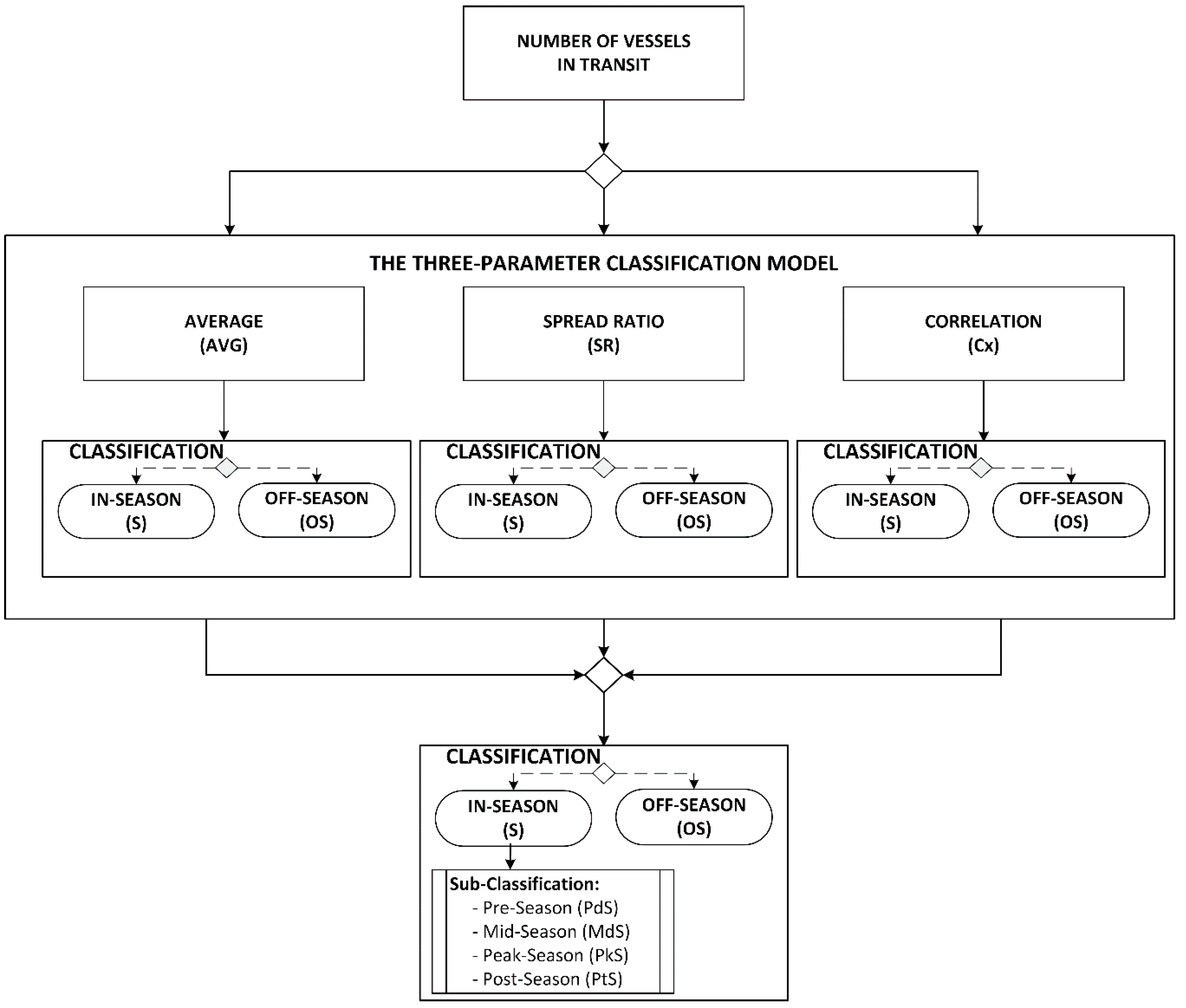
Standard statistical metrics such as expectation or the average value (AVG), standard deviation (STD), standard error (SE), and correlation coefficient (Cx) are used to study random variables. The Three-Parameter Classification Model of seasonality with the classification method has been presented in Figure 1.
From Figure 1, it can be seen that the number of vessels is an input variable in the Three-Parameter Classification Model of seasonal fluctuations. The output variables of the model block calculate a correlation, an average, and a spread ratio coefficient. The output variables are the input variables for a classification block, where the process of classification is performed. The classification process is divided into two clusters: in-season, and off-season. Every coefficient obtained from operations mentioned above is assigned either an in-season (S) or an off-season (OS) tag. That means every month has three classifier tags; a final classification for the observed month is obtained by counting assigned tags.
In the following section, mathematical foundations used in this research paper, together with their associated references, will be presented. If the random variables are considered, a vector notation can be used to describe them as follows:
where represents the month random variables with 21 data samples obtained from 1998 to 2018.
Standard statistical metrics, such as expectation or the average value, standard deviation, standard error, and correlation coefficient, are used to study random variables. The average value of the random variable x or the expectation are represented by the equation [40]:
where represents the expectation of a random variable , and N is the number of measurement samples. The standard deviation of the random variable is described with the following equation [40,41]:
where σx represents the standard deviation of the random variable . Another statistical metric used in the analysis is the standard error, SE. The standard error is defined using the following equation [41]:
where represents a standard deviation of variable , and N represents a number of measurements. Another measure that is defined is the spread ratio (SR). The spread ratio is the ratio between standard error and the sample average, as in Equation (5). It shows the spread of the population average.
The transformation of coordinates from one coordinate system to another one is shown by the equation [41]
where and are transformed coordinates of random variables and .
The statistical metric used to quantify the similarity and/or dependence among variables, and is the correlation coefficient between random variables. The correlation coefficient is calculated from the following equation [41]:
where represents the correlation coefficient, N is the number of measurements, and and represent the standard deviations of the random variables and . Furthermore, for the analysis purpose, a model matrix A is created using the following equation:
where vectors are of random independent variables, together with Equation (8), transformed into the correlation matrix Cx into the equation
The example from Equation (7), the correlation matrix has dimensions (12 × 12), as follows:
The correlation matrix shows the correlations between the variables. Finally, a trend or moving average operation on raw data needs to be performed in order to be able to get correlations between months. There are a lot of moving average algorithms available to perform the smoothing, such as a simple moving average (SMA), a weighted moving average (WMA), an exponential moving average (EMA), and an exponential weighted moving average (EWMA). An equation to perform moving average (SMA) filtering on data and to smooth data following equation is defined [40]:
where denotes the moving-average filtering of a vector x. A moving-average filter slides a window of length () along the data and computes averages of the data contained in the window size.
3. Results
Data is collected from the Croatian Bureau of Statistics (CBS), referring to the capacity and turnover of nautical ports (marina, anchorage, land marina, mooring) [15,16,17]. To investigate seasonal oscillations of nautical demand, this paper analyzes the data referring to the number of sport and recreational vessels in transit for a period of 21 years (from 1998 to 2018) as shown in Table 1.
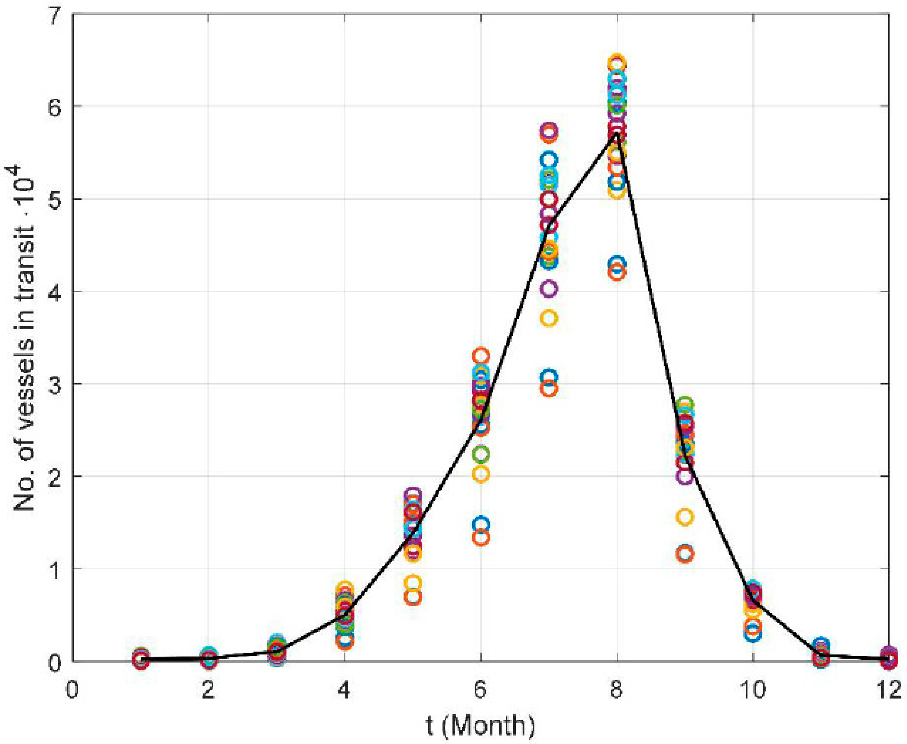
Table 1 shows the obtained data of the number of vessels in transit from 1998 to 2018 during the twelve months. The table shows a total of 252 obtained data. The data can be observed vertically, i.e., yearly, and horizontally, i.e., monthly. If the table is observed monthly, then data can be represented as a 12 by 21 matrix; otherwise, the data can be represented with a 21 by 12 matrix. Due to the fact that the research topic is to investigate the seasonal fluctuations in nautical demand, data can be processed monthly. To gain further insight into the data, Figure 1 shows the graphical representation of vessels in transit (ordinate) in the months (abscise).
Twenty-one circles (Figure 2) represent the number of vessels in transit from 1998 to 2018 for each month in a nautical year. The solid black line represents the curve obtained by taking the average value for the months. Considering the average line from January to August, there is an exponential rise in the number of vessels (approx.), and from August to December, there is an exponential decrease in the number of vessels in transit. August is the month with the highest number of vessels in transit, and therefore it is the peak month of the nautical season. Thus, in the study, August could be taken as a reference point for the in-season period. Contrary, it is evident that January, February, November, and December are months with the lowest average number of vessels in transit, which could be classified as an off-season period of a nautical year. January is the month with the lowest number of vessels in transit over the year; therefore it is a reference point for the off-season period. Furthermore, to create the Three-Parameter Classification Model of seasonality, it is necessary to apply statistical analysis of data such as average, standard deviation, standard error, spread ratio, and percentage of total averages (Table 2).
From Table 2, the statistical measure of the average, standard deviation, standard error, spread ratio, the minimal and maximal number of vessels, and a total sum percentage on average of each month are obtained. From the average values, it is evident that the months from May to September have one or two orders greater values than the other months. For example, in August, there are, on average, 57,166 vessels in transit. The minimal number of vessels in 21 years was 42,067, and the maximal number of vessels was 57,403. In June, there are 47,064 vessels in transit, with 29,499 and 57,403 as the minimum and maximum values for the vessels. In January, on average, there are 243 vessels in transit, which lies between 25 and 642 vessels. The statistical parameter average (AVG) defines the first parameter of the Tree-Parameter Classification Model necessary to determine seasonal fluctuations in demand. The spread ratio coefficient, SR, that constitutes the second parameter of the model, shows that months from April to October have lower SRs than the other months. Additionally, it can be seen (Table 2) that the AVG values for every month come from different population distribution sources. Furthermore, the SE (standard error) parameter shows the deviation of calculated AVG from the population AVG. Taking the ratio between SE and AVG for every month gives another independent variable (defined as SR) to create the second classification parameter of the model. The SR variable “catches” the local patterns in each month, i.e., shows how much (as a percentage) we can expect that the sample average value could change in the observed year (variations in the observed month). The spread ratio coefficient, SR, that constitutes the second parameter of the model, shows that it is evident that the months from April to October have lower SRs than the other months.
However, it should be noted that changes in demand, i.e., the number of vessels in transit (ViT), in the off-season months compared to the in-season months is significantly lower. The values for January are min 25, max 642, and AVG 243, and for August min 42,067; max 64,707; and AVG 57,166, as reference point months. Although the parameter SR depends on the AVG parameter, it is observed that in the in-season part of the year, it varies less than in the off-season part.
Therefore, the problem of variations in the SR parameter over the observed period does not change the determined seasonal pattern of the nautical year. It can be noticed that the proposed Three-Parameter Classification Model represents a good starting point for conducting further research on seasonality phenomena.
ANOVA analysis [40,41] has been performed on months to justify using parameter AVG as the parameter of the proposed model, as it is shown in Table 3.
Table 3 shows an ANOVA analysis of obtained monthly averages. ANOVA analysis was performed in the Microsoft Excel 2019 application. The H0 hypothesis would be that all AVGs come from the same population, and the H1 hypothesis would be that all AVGs do not come from the same population. From the table, for p-value, it is evident that the AVG values for all months do not come from the same population, and therefore the H0 hypothesis is rejected. That means the parameter AVG is acceptable as an independent variable for classification as the first parameter of the Three-Parameter Classification Model.
A graphical presentation of the variable number of vessels in transit over the twelve months is presented in Figure 3.
Raw data are designated with blue circles (Figure 3). Then a trend analysis is performed using a simple moving average (SMA) algorithm to smooth data and to prepare data for performing a correlation algorithm. A five-point window length has been chosen in the moving average algorithm. The period of five years is long enough to show a seasonal pattern and trend in nautical demand. For example, the global economic crisis was in 2008, and Croatia became a member of the EU in 2013, which yields five years [1,2,3,31]. The graphical representations (Figure 3) are of different shapes. For example, from the trend analysis, in January (1st month), from 1998 to 2005, the number of vessels is constant, or there is a small rise. From 2005 to 2008, there is a rise in the number of vessels in transit. From 2009 to 2018, there is a constant small decrease in the number of vessels in transit. On the other hand, in September (9th month), from 1998 to 2018, there is a rise in the function trend. From 2009 to 2012, there is a small stagnation or decrease in the trend.
The third parameter of the model is obtained from the full correlation matrix (Table 4). To form the correlation matrix, using Equations (7), (9), and (10), raw data are presented separately for all twelve months over a period of 21 years. Then a trend analysis is performed using Equation (11) by a moving average algorithm with a five-point window length.
In Table 4, a full correlation matrix is calculated. Horizontal and vertical fields present months. The correlation coefficient value in intersections between row and column fields with the same month is one (i.e., 100%, Table 4). A correlation coefficient on the intersection between the second row and first column determines a correlation coefficient between the January and February functions. Alternatively, a correlation coefficient is obtained by performing a correlation between the February and January functions. Therefore, correlation coefficients and are the same, i.e., That means a correlation matrix has the same values above and below the main diagonal.
4. Discussion
Studying the parameters, mean, spread ratio, and correlation coefficients from the correlation matrix on the seasonal character of recreational boating demand, conclusions can be drawn as follows. The analysis of the average parameter shows that the months from May to September have an order of magnitude greater values than the average values in the other months. These months are characterized as in-season months, whereas the other months are characterized as off-season months. In the spread ratio parameter, the months from April to October are characterized as in-season months and the other months are characterized as off-season months. The boating season lasts from April to October [30]. From the third parameter of the model, the correlation matrix (1st column), it can be observed that January, February, March, April, November, and December (Table 4) have very strong correlations that fall into the off-season period. Contrary, August (8th column) has a very strong correlation with months from May to July and a strong correlation with September and October. Months from May to October are considered as in-season months. The 4th row shows that April strongly correlates with all months except with September and October. Table 5 summarizes the previous discussion.
All three parameters have defined criteria to assign months as in-season or off-season, so it is possible to make a classification and sub-classification of the months in a nautical year. According to the proposed model (Table 5), a nautical year can be divided as in-season (S) from April to October, and off-season (OS) from January to March, as well as November and December. Furthermore, the in-season part consists of the pre-season (PdS), mid-season (MdS), peak-season (PkS), and post-season (PtS). Additionally, a definite conclusion cannot be drawn as to whether to classify April as an in-season or off-season month. From the first parameter, it is clear that April falls in the off-season part since it has almost the same number of vessels in transit as October. From the second parameter, it is evident that April can be classified either as in-season or as off-season month. From the third parameter, April correlates well with all months, so using the correlation parameter, a clear conclusion cannot be drawn. Furthermore, an ANOVA analysis has been performed to justify the usage of proposed variables in building the Three-Parameter Classification Model. First, taking into account all three variables (AVG, SR, and Cx), the following statistical measures are obtained: F = 7.08, Fcrit = 3.284, and p = 0.002764 * (with α set to 0.05). The derived measures show that the p-parameter is significant, which confirms there are no hidden correlations between variables in building the model. Next, a standard t-test is performed on clusters in-season (S), and off-season (OS), which is summarized in Table 6.
Table 6 shows t-test analysis performed on variables AVG, SR, and Cx. The analysis is performed for two cases. In the first case, the OS cluster includes April, so the S cluster contains May, July, June, August, September, and October, and the OS cluster consists of the remaining months. In the second case, April is included in the S cluster, and then the t-test is performed. The table shows that for all proposed variables, parameter p (one-tail or two-tail) is significant, which implies the relevance of the two-cluster classification.
The classification and sub-classification procedure of the proposed model have been compared by automatic classification (k-means algorithm). Figure 4 shows the two-stage classification and sub-classification of the nautical season using the k-means classification algorithm with the proposed parameters, i.e., AVG, SR, and Cx.
From the left view of Figure 4, it can be observed there are three clusters (black dotted-line circles). The first cluster consists of two months, June and August, the second cluster consists of five months, April, May, July, September, and October. The third cluster consists of four months, January, February, March, and December. In contrast to these three clusters, the k-means algorithm classified the months into the two groups, the in-season and the off-season cluster. The algorithm classifies months from May to September as in-season (S) months (red dots), and classifies the other months as off-season (OS) months (blue dots).
Furthermore, the algorithm classifies April and October as off-season (OS) months, which is an area between the in-season (S) and off-season (OS) areas. On the contrary, the proposed Three-Parameter Classification Model classifies October is as in-season (S) month. From the data, it can be seen that out of three parameters in the model, an AVG parameter classifies October as an OS month, while SR and Cx parameters classify it as an S month. Therefore, it can be observed an additional analysis of October should be conducted. At the same time, looking at the proposed model, April could be classified either as an S or OS month, and the same observation for October can be drawn. So, performing a k-means algorithm for the second time on the off-season cluster (blue dots from the left figure) separates April and October (green dots) from the rest of the months, as shown in Figure 4 right.
Although this paper focuses on the seasonal characteristics of recreational boating demand for transit berths in the Croatian Nautical Port System (CNPS), the proposed model could be used as a control and monitoring measure in the seasonal analysis of any nautical port or other maritime/tourism organization facing a diverse concentration of demand over the year. This model could be applied in any other nautical destination as long as sufficiently disaggregated data are available [17].
Compared to other well-established countries in the Mediterranean nautical tourism market, Croatia is a relatively new competitor [10], seeking to reach the position of the market leader in the region [1,2,3], and developing policies that could foster sustainable business and economy [10]. The Mediterranean, which is a very desirable destination for recreational boating, attracts many investors, especially in the eastern region. Thus, Paker and Ceren [19] state that Croatia has become, along with other East-Mediterranean countries (e.g., Montenegro, and Greece), a strong competitor to West-Mediterranean countries (e.g., France, Italy, and Spain). Recreational boating is perceived as one of the most propulsive types of tourism and has recorded the highest development rates in the Croatian economy [6,10,12]. Jugović et al. [6] point out that the existing models and plans related to the development of nautical tourism ports do not provide systematic qualitative and quantitative growth.
5. Conclusions
This paper aimed to investigate the seasonality of the recreational boating demand in nautical ports over the year, as one of the crucial problems to be studied concerning the sustainability issues of the sector.
The results of this research show that the input variable ViT is suitable for studying seasonality fluctuations in nautical demand.
The research on seasonal variations depends on the selection of the parameters which contain hidden and visible information on seasonality. The Tree-Parameter Classification Model is created by choosing the following parameters: average (AVG), spread ratio (SR), and correlation matrix (Cx). The results show that out of all investigated variables, the chosen three variables (AVG, SR, and Cx) contain the local patterns that are suitable to research and determine seasonality patterns. The selected three variables are independent among themselves (proved with ANOVA). The AVG variable shows the sample mean values of ViT every month over 21 years (from 1998 to 2018). The SR variable determines the local patterns of each month, i.e., it shows how much change could be expected in the sample average value. The Cx variable shows correlations between months over the year. The proposed model is created on the example of the Croatian nautical ports.
The proposed model classifies a nautical year into two main periods: in-season (months from May to October) and off-season (January to March, and November and December). Furthermore, the in-season period is classified into pre-season (May), mid-season (June and September), peak-season (July and August), and post-season (October).
Also, there is the question of the month of April. According to the proposed model, it could be placed either in the off-season or in the in-season period (cluster). Based on the circumstances of the particular nautical year, further investigation of the pre-season period is recommended to classify April.
The model could be used in practical applications, which is an additional contribution to the research. According to the results of the study, the proposed Three-Parameter Classification Model could broadly be used as an analytical framework in developing strategic plans for countries with a strong maritime and tourist orientation (e.g., Croatia, Montenegro, Greece, and Turkey). The proposed model could notably be used as a scientific application in creating seasonal strategies.
Further research should include more variables that can affect organizational performance and enable the development of a more robust model.
Author Contributions
Conceptualization, E.M. and J.Š.; methodology, E.M., J.Š., and M.K.; software, J.Š.; validation, E.M., J.Š. and M.K.; formal analysis, E.M. and M.K.; investigation, E.M.; writing—original draft preparation, E.M., J.Š. and M.K.; visualization, E.M., J.Š. and M.K. All authors have read and agreed to the published version of the manuscript.
Funding
This research received no external funding.
Conflicts of Interest
The authors declare no conflict of interest.
References
- Ministry of Sea, Transport and Infrastructure. Maritime Development and Integrated Maritime Policy Strategy of the Republic Of Croatia for the Period from 2014 to 2020. Zagreb. 2014. (OG 93/14). Available online: http://www.csamarenostrum.hr/userfiles/files/Nacion%20zakon%20engl/MDIMPSRC.pdf (accessed on 19 June 2020).
- Ministry of Sea, Transport and Infrastructure; Ministry of Tourism. Nautical tourism development strategy of the Republic of Croatia 2009–2019. Zagreb; 2008. Available online: https://mmpi.gov.hr/UserDocsImages/arhiva/Strategija%20razvoja%20nautickog%20turizma%20ENGL%201.pdf (accessed on 21 June 2020).
- The Government of the Republic of Croatia. Tourism Development Strategy of the Republic of Croatia until 2020. Republic Of Croatia; Ministry Of Tourism. Zagreb. 2013. (Official Gazette, No. 55/2013). Available online: https://mint.gov.hr/UserDocsImages/arhiva/Tourism_development_strategy_2020.pdf (accessed on 21 June 2020).
- Kovačić, M.; Gračan, D.; Jugović, A. The scenario method of nautical tourism development—a case study of Croatia. Pomorstvo 2015, 29, 125–132. [Google Scholar]
- Marušić, Z.; Ivandic, N.; Horak, S. Nautical Tourism within TSA Framework: Case of Croatia. In Proceedings of the 13th Global Forum on Tourism Statistics, Nara, Japan, 17–18 November 2014. [Google Scholar]
- Jugović, A.; Kovačić, M.; Hadžić, A. Sustainable development model for nautical tourism ports. Tour. Hosp. Manag. 2011, 17, 175–186. [Google Scholar]
- European Commission. Directorate-General for Maritime Affairs and Fisheries: Assessment of the Impact of Business Development Improvements around Nautical Tourism; Final report; European Union: Brussels, Belgium, 2017; ISBN 978-92-79-67732-8. [Google Scholar]
- Lam-González, Y.E.; Suárez-Rojas, C.; León, C.J. Factors Constraining International Growth in Nautical Tourism Firms. Sustainability 2019, 11, 6846. [Google Scholar] [CrossRef] [Green Version]
- Sariisik, M.; Turkayb, O.; Akov, O. How to manage yacht tourism in Turkey: A SWOT analysis and related strategies. In Proceedings of the 7th International Strategic Management Conference, Paris, France, 30 June–2 July 2011; Volume 24, pp. 1014–10257. [Google Scholar]
- Moreno, M.J.; Otamendi, F.J. Fostering Nautical Tourism in the Balearic Islands. Sustainability 2017, 9, 2215. [Google Scholar] [CrossRef] [Green Version]
- Ioannidis, S.A.K. An overview of Yachting Tourism and its role in the development of coastal areas of Croatia. J. Hosp. Tour. Issues 2019, 1, 30–43. [Google Scholar]
- Kovacic, M.; Favro, S.; Mezak, V. Construction of Nautical Tourism Ports as an Incentive to Local Development. Environ. Eng. Manag. J. 2016, 15, 395–403. [Google Scholar]
- Lukovic, T. (Ed.) Nautical Tourism; CAB International: Croydon, UK, 2013. [Google Scholar]
- Gon, M.; Osti, L.; Pechlaner, H. Leisure boat tourism: Residents’ attitudes towards nautical tourism development. Tour. Rev. 2016, 71, 180–191. [Google Scholar] [CrossRef]
- Croatian Bureau of Statistics. First Release (2010–2018): Nautical Tourism Capacity and Turnover of Ports; Croatian Bureau of Statistics: Zagreb, Croatia, 2019; ISSN 1330-0350. [Google Scholar]
- Croatian Bureau of Statistics. First Release (2003–2009): Nautical Tourism Capacity and Turnover of Ports; Croatian Bureau of Statistics: Zagreb, Croatia, 2010; ISSN 1334-0565. [Google Scholar]
- Croatian Bureau of Statistics. First Release (1998–2002): Nautical Tourism Capacity and Turnover of Ports; Croatian Bureau of Statistics: Zagreb, Croatia, 2003; ISSN 1330-0350. [Google Scholar]
- Gračan, D.; Gregorić, M.; Martinić, T. Nautical tourism in Croatia: Current situation and outlook. In Proceedings of the Tourism & Hospitality Industry, Opatija, Hrvatska, 28–29 April 2016; pp. 66–79. [Google Scholar]
- Paker, N.; Vural, C.A. Customer segmentation for marinas: Evaluating marinas as destinations. Tour. Manag. 2016, 56, 156–171. [Google Scholar] [CrossRef]
- Raviv, A.; Yedidia, S.; Weber, T.Y. Strategic planning for increasing profitability: The case of marina industry. EuroMed. J. Bus. 2009, 4, 200–214. [Google Scholar] [CrossRef]
- Kožić, I.; Krešić, D.; Boranić-Živoder, S. Analiza sezonalnosti turizma u Hrvatskoj primjenom metode Gini koeficijenta. Ekonomski Pregled 2013, 64, 159–182. [Google Scholar]
- Martin Rojo, I. Economic development versus environmental sustainability: The case of tourist marinas in Andalusia. Eur. J. Tour. Res. 2009, 2, 162–177. [Google Scholar]
- Balaguer, P.; Diedrich, A.; Sardá, R.; Fuster, M.; Cañellas, B.; Tintoré, J. Spatial analysis of recreational boating as a first key step for marine spatial planning in Mallorca (Balearic Islands, Spain). Ocean Coast Manag 2011, 54, 241–249. [Google Scholar] [CrossRef]
- Kovačić, M.; Favro, S.; Staftić, D. Comparative analysis of Croatian and Mediterranean nautical tourism ports. In Proceedings of the 2nd International Scientific Conference, Advances in Hospitality and Tourism Marketing and Management Conference, Corfu, Greece, 31 May–3 June 2012; pp. 1–7. [Google Scholar]
- Duro, J.A. Seasonality of hotel demand in the main Spanish provinces: Measurements and decomposition exercises. Tour. Manag. 2016, 52, 52–63. [Google Scholar] [CrossRef] [Green Version]
- De Cantis, S.; Ferrante, M.; Vaccina, F. Seasonal pattern and amplitude—A logical framework to analyse seasonality in tourism: an application to bed occupancy in Sicilian hotels. Tour. Econ. 2011, 17, 655–675. [Google Scholar] [CrossRef]
- Higham, J.; Hinch, T. Tourism, sport, and seasons: The challenges and potential of overcoming seasonality in the sport and tourism sectors. Tour. Manag. 2002, 23, 175–185. [Google Scholar] [CrossRef]
- Fernández-Morales, A. Tourism Mobility in Time and Seasonality in Tourism. RIEDS 2017, 35–52. Available online: https://www.semanticscholar.org/paper/Tourism-mobility-in-time-and-seasonality-in-tourism-Morales/b0b6802c191050e414bd4add9bbb7dd1faf4faa8 (accessed on 19 June 2020).
- Fernández-Morales, A.; Cisneros-Martínez, J.D.; McCabe, S. Seasonal concentration of tourism demand: Decomposition analysis and marketing implications. Tour. Manag. 2016, 56, 172–190. [Google Scholar] [CrossRef]
- European Commission. Study on Specific Challenges for Sustainable Development of Coastal and Maritime Tourism in Europe; Final Report; European Union: Brussels, Belgium, 2016; ISBN 978-92-9202-190-0. [Google Scholar]
- ECORYS. Study in Support of Policy Measures for Maritime and Coastal Tourism at EU Level; Final Report; European Commission: Brussels, Belgium, 2013. [Google Scholar]
- Kovačić, M.; Gržetić, Z.; Bosković, D. Nautical tourism in fostering the sustainable development: A case study of Croatia’s coast and Island. Tourismos 2011, 6, 221–232. [Google Scholar]
- Favro, S.; Gržetić, Z.; Kovačić, M. Towards sustainable yachting in Croatian traditional island ports. Environ. Eng. Manag. J. 2010, 9, 787–794. [Google Scholar] [CrossRef]
- Diakomihalis, M.N.; Lagos, D.G. Estimation of the economic impacts of yachting in Greece via the tourism satellite account. Tour. Econ. 2008, 14, 871–887. [Google Scholar] [CrossRef]
- Jovanovic, T.; Dragin, A.; Armenski, T.; Pavic, D.; Davidovic, N. What demotivates the tourist? Constraining factors of nautical tourism. J. Trav. Tour. Mar. 2013, 30, 858–872. [Google Scholar] [CrossRef]
- Song, H.; Li, G. Tourism demand modelling and forecasting—A review of Recent research. Tour. Manag. 2008, 29, 203–220. [Google Scholar] [CrossRef] [Green Version]
- Song, H.; Witt, S.F.; Wu, D.C. An Empirical Study of Forecast Combination in Tourism. J. Hosp. Tour. Res. 2009, 1, 3–29. [Google Scholar] [CrossRef] [Green Version]
- Lundtorp, S. Measuring tourism seasonality. In Seasonality in Tourism; Baum, T., Lundtorp, S., Eds.; Pergamon: Oxford, UK, 2001. [Google Scholar]
- Koenig-Lewis, N.; Bischoff, E.E. Seasonality research: the state of the art. Int. J. Tour. Res. 2005, 7, 201–219. [Google Scholar] [CrossRef]
- Strang, G. Linear Algebra and Learning from Data; Wellesley-Cambridge Press: Wellesley, MA, USA, 2019. [Google Scholar]
- Pavli&ć, I. Statistička Teorija i Primjena; Tehnička knjiga Zagreb: Zagreb, Yugoslavia, 1988. [Google Scholar]
Figure 1.
The Three-Parameter Classification Model of seasonal fluctuations with the classification method.
Figure 1.
The Three-Parameter Classification Model of seasonal fluctuations with the classification method.

Figure 2.
Graphical presentation of the number of vessels in transit vs. months.

Figure 3.
Graphical presentation of the number of vessels in transit through months over the years.
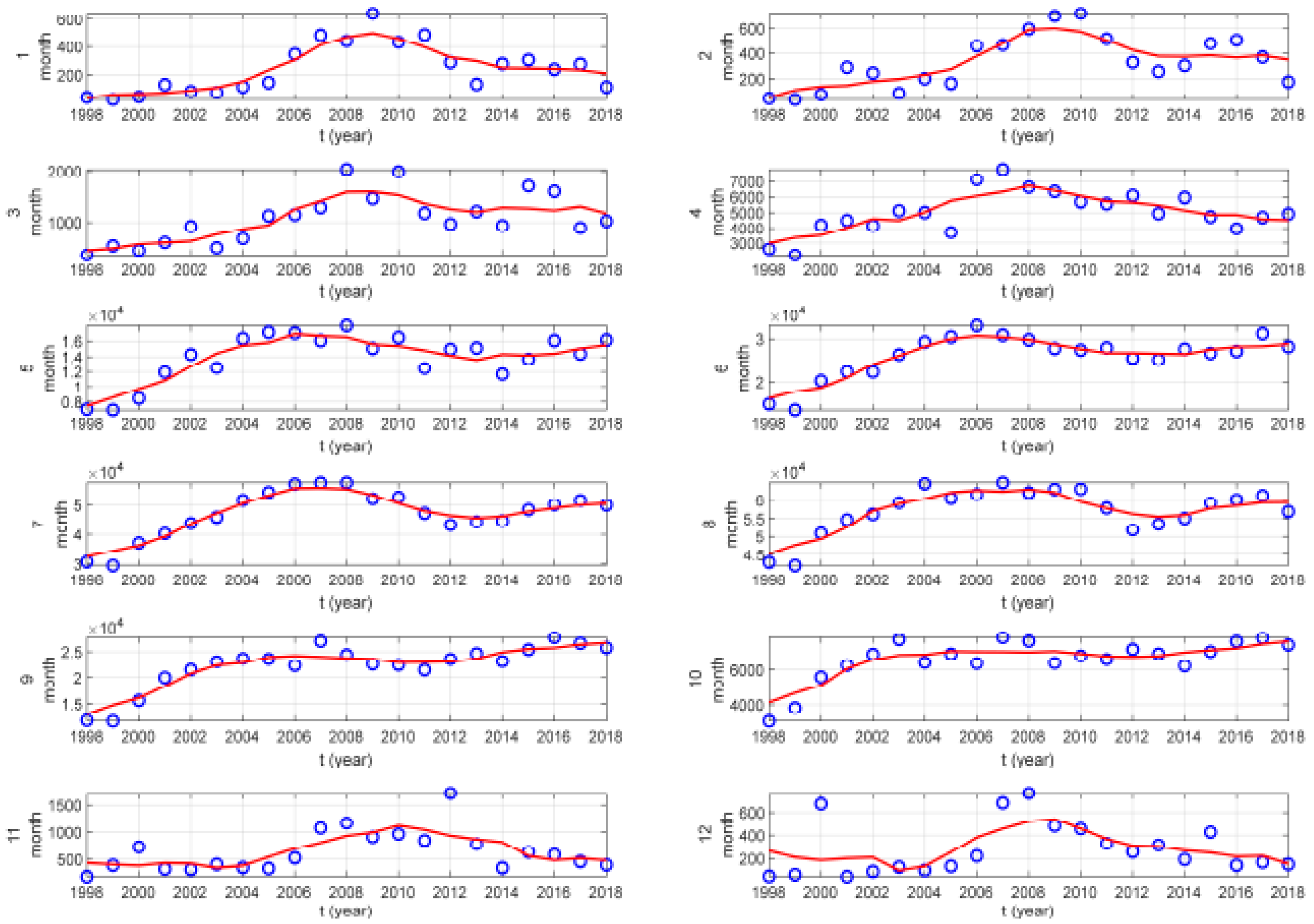
Figure 4.
Classification and sub-classification of the nautical season using a k-means algorithm.


Table 1.
The number of vessels in transit (ViT) from 1998 to the 2018 year categorized in twelve months.
Table 1.
The number of vessels in transit (ViT) from 1998 to the 2018 year categorized in twelve months.
| Vessels in Transit (ViT) | |||||||||||
|---|---|---|---|---|---|---|---|---|---|---|---|
| Y/M | 1998 | 1999 | 2000 | 2001 | 2002 | 2003 | 2004 | 2005 | 2006 | 2007 | 2008 |
| I | 40 | 25 | 44 | 130 | 82 | 75 | 115 | 145 | 346 | 483 | 441 |
| II | 44 | 35 | 73 | 288 | 243 | 84 | 199 | 162 | 458 | 466 | 595 |
| III | 336 | 525 | 432 | 594 | 918 | 486 | 674 | 1127 | 1148 | 1286 | 2035 |
| IV | 2587 | 2182 | 4194 | 4499 | 4164 | 5119 | 5006 | 3719 | 7130 | 7808 | 6637 |
| V | 7033 | 6944 | 8460 | 11924 | 14292 | 12523 | 16303 | 17108 | 17011 | 16051 | 17951 |
| VI | 14782 | 13410 | 20264 | 22411 | 22352 | 26441 | 29300 | 30441 | 32994 | 30838 | 29805 |
| VII | 30697 | 29499 | 37086 | 40270 | 43772 | 45835 | 51576 | 54206 | 56922 | 57367 | 57403 |
| VIII | 42924 | 42067 | 50906 | 54638 | 56125 | 59314 | 64421 | 60430 | 61553 | 64707 | 61992 |
| IX | 11728 | 11578 | 15617 | 19992 | 21516 | 23065 | 23659 | 23585 | 22346 | 27020 | 24397 |
| X | 3037 | 3812 | 5580 | 6257 | 6896 | 7746 | 6418 | 6911 | 6372 | 7866 | 7657 |
| XI | 191 | 394 | 722 | 327 | 316 | 409 | 352 | 337 | 525 | 1074 | 1169 |
| XII | 51 | 65 | 674 | 48 | 91 | 128 | 101 | 135 | 221 | 682 | 767 |
| Vessels in Transit (ViT) | |||||||||||
| Y/M | 2009 | 2010 | 2011 | 2012 | 2013 | 2014 | 2015 | 2016 | 2017 | 2018 | |
| I | 642 | 433 | 486 | 287 | 133 | 277 | 305 | 238 | 275 | 114 | |
| II | 702 | 721 | 514 | 328 | 255 | 303 | 478 | 504 | 369 | 174 | |
| III | 1459 | 1990 | 1175 | 965 | 1209 | 933 | 1704 | 1598 | 890 | 1025 | |
| IV | 6356 | 5686 | 5562 | 6092 | 4939 | 5955 | 4735 | 3959 | 4695 | 4918 | |
| V | 15058 | 16434 | 12456 | 14957 | 15128 | 11666 | 13670 | 16058 | 14366 | 16136 | |
| VI | 27832 | 27492 | 28002 | 25591 | 25260 | 27730 | 26759 | 27220 | 31207 | 28249 | |
| VII | 52034 | 52556 | 47173 | 43262 | 44280 | 44595 | 48380 | 50032 | 51494 | 49919 | |
| VIII | 62901 | 63005 | 57808 | 51845 | 53396 | 55024 | 59205 | 60101 | 61241 | 56898 | |
| IX | 22602 | 22452 | 21486 | 23547 | 24648 | 23148 | 25399 | 27743 | 26618 | 25763 | |
| X | 6392 | 6801 | 6605 | 7181 | 6916 | 6229 | 7052 | 7638 | 7838 | 7441 | |
| XI | 905 | 961 | 842 | 1720 | 776 | 346 | 629 | 581 | 461 | 400 | |
| XII | 482 | 457 | 328 | 255 | 314 | 192 | 427 | 143 | 169 | 151 | |
Table 2.
Statistical measures as seasonal indicators in nautical demand.
| Month (M). | Min | Max | Average [AVG] | Standard Deviation [STD] | Standard Error [SE] | Spread Ratio SR [%] |
|---|---|---|---|---|---|---|
| I | 25 | 642 | 243 | 176.03 | 38.41 | 15.77 |
| II | 35 | 721 | 333 | 207.91 | 45.37 | 13.62 |
| III | 336 | 2035 | 1071 | 487.37 | 106.35 | 9.92 |
| IV | 2182 | 7808 | 5044 | 1379.58 | 301.05 | 5.97 |
| V | 6944 | 17951 | 13882 | 3203.55 | 699.07 | 5.04 |
| VI | 13410 | 32994 | 26113 | 5041.39 | 1100.12 | 4.21 |
| VII | 29499 | 57403 | 47064 | 7866.26 | 1716.56 | 3.65 |
| VIII | 42067 | 64707 | 57166 | 6279.89 | 1370.39 | 2.40 |
| IX | 11578 | 27743 | 22281 | 4396.12 | 959.31 | 4.31 |
| X | 3037 | 7866 | 6602 | 1226.97 | 267.75 | 4.06 |
| XI | 191 | 1169 | 606 | 292.78 | 63.89 | 10.53 |
| XII | 48 | 767 | 251 | 205.89 | 44.93 | 17.89 |
Table 3.
ANOVA analysis performed on months.
| Source of Variation | SS | df | MS | F | p-Value | F crit |
|---|---|---|---|---|---|---|
| Between Months | 9 × 10¹⁰ | 11 | 8 × 10⁹ | 600.98 | 9 × 10−168 ** | 1.8287 |
| Within Months | 3 × 10⁹ | 240 | 1 × 10⁷ | |||
| Total | 9 × 10¹⁰ | 251 |
Note: ** significant (p < 0.01), where SS is the sum of squares, df is a degree of freedom, MS is a mean square parameter, F is the parameter for f-statistics (obtained as the ratio between the mean of the sum of squares between months (MSSB) and the mean of the sum of squares within months (MSSW), p is the probability parameter (α = 0.05), F crit is the critical parameter for F-statistics.
Table 4.
A full correlation matrix, , with coefficients between the months.
| Mo. | I | II | III | IV | V | VI | VII | VIII | IX | X | XI | XII |
|---|---|---|---|---|---|---|---|---|---|---|---|---|
| I | 100 | 98.09 | 94.53 | 91.87 | 73.85 | 72.18 | 76.03 | 69.38 | 60.16 | 59.65 | 97.78 | 98.32 |
| II | 98.09 | 100 | 97.97 | 88.49 | 76.73 | 75.33 | 77.10 | 71.42 | 69.30 | 68.30 | 94.90 | 94.37 |
| III | 94.53 | 97.97 | 100 | 86.17 | 81.34 | 81.38 | 81.12 | 74.49 | 78.70 | 75.45 | 89.81 | 90.84 |
| IV | 91.87 | 88.49 | 86.17 | 100 | 86.70 | 84.84 | 88.26 | 84.94 | 67.35 | 70.33 | 88.27 | 92.50 |
| V | 73.85 | 76.73 | 81.34 | 86.70 | 100 | 98.88 | 98.56 | 97.78 | 89.77 | 92.23 | 64.18 | 71.05 |
| VI | 72.18 | 75.33 | 81.38 | 84.84 | 98.88 | 100 | 97.99 | 96.71 | 92.90 | 93.78 | 61.60 | 69.13 |
| VII | 76.03 | 77.10 | 81.12 | 88.26 | 98.56 | 97.99 | 100 | 98.46 | 85.35 | 87.77 | 64.99 | 75.07 |
| VIII | 69.38 | 71.42 | 74.49 | 84.94 | 97.78 | 96.71 | 98.46 | 100 | 84.72 | 89.64 | 57.99 | 67.96 |
| IX | 60.16 | 69.30 | 78.70 | 67.35 | 89.77 | 92.90 | 85.35 | 84.72 | 100 | 98.03 | 50.12 | 53.50 |
| X | 59.65 | 68.30 | 75.45 | 70.33 | 92.23 | 93.78 | 87.77 | 89.64 | 98.03 | 100 | 49.75 | 53.18 |
| XI | 97.78 | 94.90 | 89.81 | 88.27 | 64.18 | 61.60 | 64.99 | 57.99 | 50.12 | 49.75 | 100 | 96.49 |
| XII | 98.32 | 94.37 | 90.84 | 92.50 | 71.05 | 69.13 | 75.07 | 67.96 | 53.50 | 53.18 | 96.49 | 100 |
Table 5.
Classification and sub-classification of the nautical season with the Three-Parameter Classification Model.
Table 5.
Classification and sub-classification of the nautical season with the Three-Parameter Classification Model.
| Three-Parameters | Months | |||||||||||
|---|---|---|---|---|---|---|---|---|---|---|---|---|
| I | II | III | IV | V | VI | VII | VIII | IX | X | XI | XII | |
| AVG | OS | OS | OS | OS | S | S | S | S | S | OS | OS | OS |
| SR | OS | OS | OS | S | S | S | S | S | S | S | OS | OS |
| Cx | OS | OS | OS | OS/S | S | S | S | S | S | S | OS | OS |
| Classification | OS | OS | OS | ? | S | S | S | S | S | S | OS | OS |
| Sub Class. | OS | OS | OS | ? | PdS | MdS | PkS | PkS | MdS | PtS | OS | OS |
Table 6.
Two cluster t-test statistics.
| Cluster 1 | Cluster 2 | Cluster 1 | Cluster 2 | |||
|---|---|---|---|---|---|---|
| Classification | OS | S | OS | S | ||
| Month (M) | 1, 2, 3, 4, 11, 12 | 5, 6, 7, 8, 9,10 | 1, 2, 3, 11, 12 | 4, 5, 6, 7, 8, 9, 10 | ||
| Variables | SR | AVG | Cx | SR | AVG | Cx |
| t Stat | −3.448 | 4.620 | −5.403 | −3.307 | 5.919 | −6.670 |
| P(T ≤ t) one-tail | 0.009 | 0.003 | 0.000 | 0.008 | 0.001 | 0.000 |
| t Critical one-tail | 2.015 | 2.015 | 1.833 | 1.943 | 2.015 | 1.833 |
| P(T ≤ t) two-tail | 0.018 | 0.006 | 0.000 | 0.016 | 0.002 | 0.000 |
| t Critical two-tail | 2.571 | 2.571 | 2.262 | 2.447 | 2.571 | 2.262 |
| α = 0.05 | ||||||
© 2020 by the authors. Licensee MDPI, Basel, Switzerland. This article is an open access article distributed under the terms and conditions of the Creative Commons Attribution (CC BY) license (http://creativecommons.org/licenses/by/4.0/).
Share and Cite
MDPI and ACS Style
Marušić, E.; Šoda, J.; Krčum, M. The Three-Parameter Classification Model of Seasonal Fluctuations in the Croatian Nautical Port System. Sustainability 2020, 12, 5079. https://doi.org/10.3390/su12125079
AMA Style
Marušić E, Šoda J, Krčum M. The Three-Parameter Classification Model of Seasonal Fluctuations in the Croatian Nautical Port System. Sustainability. 2020; 12(12):5079. https://doi.org/10.3390/su12125079
Chicago/Turabian StyleMarušić, Eli, Joško Šoda, and Maja Krčum. 2020. "The Three-Parameter Classification Model of Seasonal Fluctuations in the Croatian Nautical Port System" Sustainability 12, no. 12: 5079. https://doi.org/10.3390/su12125079
Note that from the first issue of 2016, this journal uses article numbers instead of page numbers. See further details here.