Remote Sensing Applications for Monitoring Terrestrial Protected Areas: Progress in the Last Decade

Abstract

Terrestrial protected areas (PAs) play an essential role in maintaining biodiversity and ecological processes worldwide, and the monitoring of PAs is a useful tool in assessing the effectiveness of PA management. Advanced remote sensing technologies have been increasingly used for mapping and monitoring the dynamics of PAs. We review the advances in remote sensing-based approaches for monitoring terrestrial PAs in the last decade and identify four types of studies in this field: land use & land cover and vegetation community classification, vegetation structure quantification, natural disturbance monitoring, and land use & land cover and vegetation dynamic analysis. We systematically discuss the satellite data and methods used for monitoring PAs for the four research objectives. Moreover, we summarize the approaches used in the different types of studies. The following suggestions are provided for future studies: (1) development of remote sensing frameworks for local PA monitoring worldwide; (2) comprehensive utilization of multisource remote sensing data; (3) improving methods to investigate the details of PA dynamics; (4) discovering the driving forces and providing measures for PA management. Overall, the integration of remote sensing data and advanced processing methods can support PA management and decision-making procedures.

1. Introduction

Protected areas (PAs) are keystones for maintaining biodiversity and ecological processes, and have been recognized as critical elements to achieve the objectives of the Convention on Biological Diversity (CBD) and the Sustainable Development Goals (SDGs) [1]. Due to environmental degradation resulting from anthropogenic influences and climate change, the number of PAs has increased significantly over the last few decades worldwide, reaching 248,330 in March 2020 [2]. According to the Protected Planet Live Report 2020 [3], the area of terrestrial PAs has slightly increased from 14.7% in 2016 to 15.1% in 2020, and the area of marine PAs has increased faster from 10.2% to 17.2% in national waters; therefore, the National Aichi target #11 commitments of 17% and 10% coverage for terrestrial and marine PAs, respectively, are likely to be achieved by 2020. Compared with the rapid progress in marine PAs, the designation of terrestrial PAs is lagging behind, and there is greater concern about qualitative evaluation elements, such as representativeness [4], connectivity [5], and management effectiveness [6,7], rather than the number of areas being designated as legal PAs [8,9,10].

Currently, many PAs are ‘paper parks’ and face serious threats [11,12] due to a lack of management and no implementation of the protection plan [13,14]. This situation is largely attributed to conflicts between the demands of local community imposed on PAs and strict protection management policies [15]. PAs are experiencing widespread degradation, downsizing, and degazettement (PADDD) events in some countries [16,17]. Apart from reducing the extent of PAs, PADDD events can also accelerate biodiversity loss and impede conservation efforts. However, it is challenging to trace these events using traditional means due to poor documentation and inadequate resources and monitoring activities in PAs [10]. The SDGs, as well as other projects, have been used to assess the effectiveness of the establishment and management of PAs [18]. Monitoring remains a key priority for the assessment of PA management [9], including the evaluation of the performance of conservation management practices and the measures of dealing with human disturbances and global climate change in the future to ensure habitat and species preservation.

In consideration of the local economic development, PAs are usually designated in remote and low accessibility sites [19], which prevents the use of traditional monitoring methods of PAs [20], such as ground patrols, observing from watchtowers, or field-based inventories, because these methods are costly and labor- and time-consuming. In contrast, remote sensing monitoring is less costly, time-consuming, and labor-intensive and more objective than field-based approaches. Extensive historical archives and multiple resolutions have provided the capability to extract long-term changes in landscape composition and function of PAs continuously from the 1970s at multiple scales. Due to a significant increase in multisource remotely sensed data and machine learning techniques [21] in recent decades, remote sensing has developed rapidly and has become an important tool for the management and monitoring of PAs in time and space [22,23]. Gillespie et al. [24] pointed out that the spaceborne remote sensing monitoring of PAs has primarily focused on forest ecosystems and land use and land cover (LULC) changes in and around PAs using time-series data in the past. Due to the relatively coarse resolution of remote sensing data in the past few decades, studies have focused either on regional or global scales [12,24,25]. However, the methods used to analyze different ecosystems and communities may vary widely, and the drivers for LULC changes and the PA management results are often time- and location-specific; therefore, local data linking human activities and strategies are needed [10].

Natural resource managers require information on local conditions in individual PAs under their management to adopt conservation strategies [26]. Reviews on this topic have been conducted from a global perspective [22,23,24,27,28]. For example, Wang et al. [22] reviewed state-of-the-art remote sensing technologies and discussed the challenges of remote sensing applications for PAs. Duan et al. [23] presented a bibliometric analysis of remote sensing research on PAs from 1991 to 2018. A review from a local perspective can provide details about major concerns and monitoring methods of PAs in various conditions, as well as information on site-specific PA management. Therefore, we conducted a systematic review of the methods used for remote sensing monitoring of individual terrestrial PAs worldwide to provide answers to the following questions:

• What are the ecosystems and topics of concern for researchers and PA managers that have been investigated using remote sensing?
• What are the preferred satellite datasets used for PA monitoring?
• What are the methods best suited for different objectives and ecosystems?
• What are the improvements required in future studies considering current remote sensing approaches?

First, we present quantitative statistics to answer research questions 1 and 2. Second, we conduct a systematic literature review to answer research question 3. Finally, we synthesize the results of the systematic review to address research question 4.

2. Systematic Literature Review

2.1. Database Search

We searched the literature in the ISI Web of Science database (available online: http://www.webofknowledge.com, accessed on 18 March 2020), focusing on the monitoring, management, and mapping studies of terrestrial PAs using remote sensing technologies. The following search string was used:

TS = (protected area OR national park * OR nature reserve *) AND TS = (remote sensing OR remotely sensed OR satellite *) AND TS = (monitoring OR management OR mapping) NOT TS = (marine) NOT TS = (global or national) AND SU = (environmental science and ecology OR forestry OR science technology). We refined the search by focusing on studies from the last decade (2010–2020) and excluded review articles, providing an initial result of 1327. (TS = Topic search, including title, abstract, author, and keywords; SU = research direction; Asterisk (*) = A wildcard for any type, number, or character.)

Then, we browsed the titles and abstracts of these studies to exclude studies that were not relevant to our review (e.g., research at a global or national scale or using remote sensing to guide fieldwork, marine, or crop research, which was irrelevant to terrestrial PAs, and other environmental studies that did not fit our objectives). We downloaded the full text of the selected studies using the following criteria and finally obtained 94 studies for our systematic review:

• The study area must be an officially designated PA with a spatially explicit boundary and a description of the PA in the paper;
• Since our focus was on individual PAs, comparative analyses between several PAs or studies of ecological corridor development between PAs were not considered;
• The method must be (semi-)automatic; therefore, we did not consider studies that used solely visual interpretation of remote sensing data;
• The research has provided insights into PA management; some experimental studies with advanced methods but limited to several small plots were not included in our review.

2.2. Information Extraction and Analysis

For each study in the collection, we extracted several attributes for analysis (

Table 1. Information extracted from the literature.

Attribute	Abbreviation	Description
PA name	-	The designated name of the PA.
Country	-	The location of the PA.
Latitude/longitude	-	Location of the PA; obtained from the study area description or, if not provided, we used Google Maps or Wikipedia to define the approximate location.
Research objectives	LVC, VSQ, NDM, LVD	The main objectives of the research: LULC/Vegetation classification (L/VC), vegetation structure quantification (VSQ), natural disturbance monitoring (NDM), and LULC/Vegetation dynamics.
Method or model	-	The method or model used for monitoring PAs to achieve the research objectives.
Remote sensing data	-	The remote sensing datasets used in the research.
Spatial resolution	C, M, H, VH, Fusion	The spatial resolution used in the study: coarse (C): ≥100 m; moderate (M): 10–100 m; high (H): 1–10 m; very high (VH): <1 m; if different datasets were integrated, “Fusion” was used.
Temporal resolution	SD, MD, D, VD	The temporal resolution of the analysis: SD: single date; MD: multidate (more than one image but less than annual; often used to represent different periods; D: dense date (annual data); VD: very dense date (intra-annual data).
Spectral resolution	SI, Multi, Hyper, SAR, LiDAR, Fusion	The spectral resolution used in the study: SI (single VI or band), Multi (multispectral VIs or bands), Hyper (hyperspectral bands), SAR (Synthetic Aperture Radar), LiDAR (Light detection and ranging); if different datasets were integrated, “Fusion” was used.
VI	-	VIs used in the studies, such as normalized difference vegetation index (NDVI), enhanced vegetation index (EVI), soil-adjusted vegetation index (SAVI), normalized burn ratio (NBR).

). Specifically, we focused on the name, location, and ecosystem of the PAs. We classified the studies into four categories based on the main research objectives. (1) LULC and vegetation community classification (LVC), i.e., the identification of major LULC, vegetation types, and extraction of key species, focusing on the application of advanced algorithms and multisource data to improve the accuracy of classification. (2) Vegetation structure quantification (VSQ), which is a crucial aspect of forest resource monitoring and PA management. (3) Natural disturbance monitoring (NDM), i.e., monitoring the extent, severity, and frequency of natural disturbances. (4) LULC and vegetation dynamic analysis (LVD), which refers to the dynamic analysis of LULC and vegetation health using classified images of LULC or time-series vegetation index (VI) products in and around a PA. This method is most commonly used for evaluating management effectiveness. We then recorded the method/model and data used in the given domain. The spatial, temporal, and spectral properties of the datasets were evaluated to summarize the satellite data used in the different studies. A detailed description of the properties is listed in Table 1.

After extracting the information from each study in the analysis, we plotted the spatiotemporal distribution of the individual PAs based on the biome classification map of Olson et al. (2001) [29]. If there was no description of latitude or longitude, we obtained the location information from Google Maps or Wikipedia. We created a statistical summary of all the sensor attributes used in the studies grouped by four types of studies.

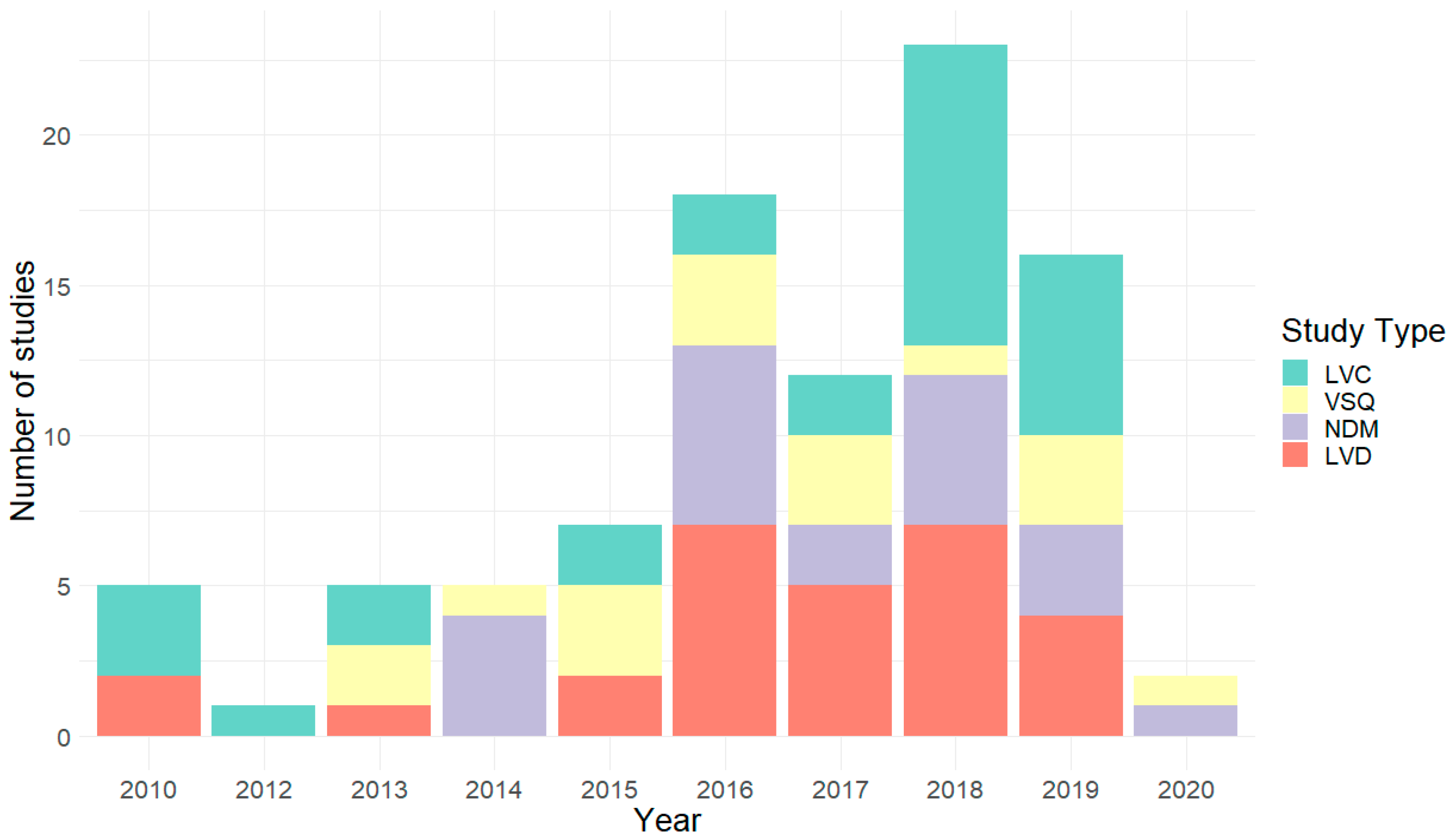
2.3. Results of the Systematic Review

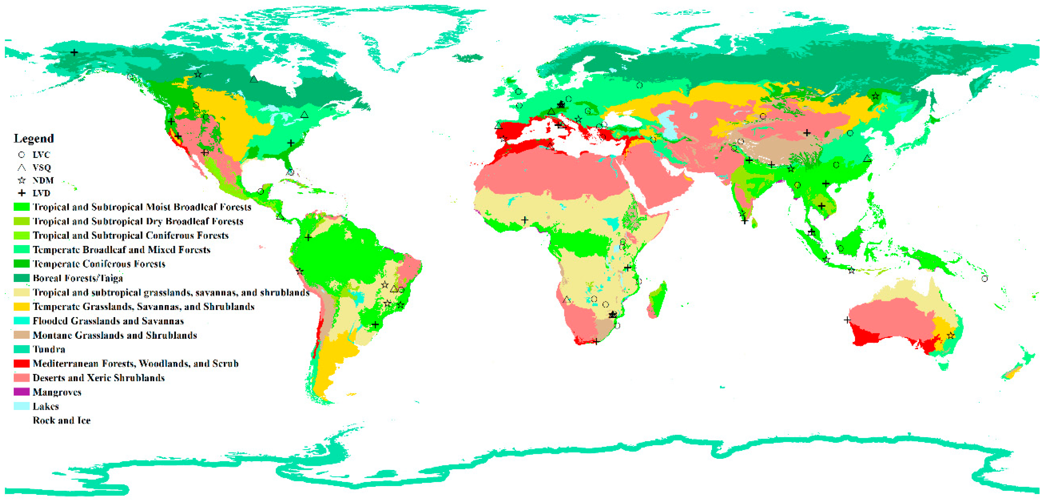
2.3.1. The Spatial Distribution of the Reviewed PAs

There are 76 PAs that were analyzed using remote sensing in our review. The Bavarian Forest National Park (BFNP, with 8 studies) in Germany and Kruger National Park (KNP, with 6 studies) in South Africa ranked first and second in terms of number of studies (Figure 1, based on [29]). The proportion of studies was similar in Europe (25.5%), Asia (25.5%), Africa (19.1%), and North America (18.1%), whereas South America (8.5%) had relatively fewer studies on this topic (Figure 1;

Table 2. The number of studies in the biomes. We classified 3 studies in Turkey and Russia into Europe to simplify the statistics.

Code	Biome	Number of Studies
		Africa	Asia	Europe	North America	Oceania	South America	Total
1	Tropical and Subtropical Moist Broadleaf Forests	3	11	0	1	1	5	21
2	Tropical and Subtropical Dry Broadleaf Forests	0	2	0	0	0	0	2
3	Tropical and Subtropical Coniferous Forests	0	0	0	0	0	0	0
4	Temperate Broadleaf and Mixed Forests	0	3	19	2	0	0	24
5	Temperate Coniferous Forests	0	2	2	4	0	0	8
6	Boreal Forests/Taiga	0	0	0	2	0	0	2
7	Tropical and Subtropical Grasslands, Savannas, and Shrublands	12	0	0	0	0	3	15
8	Temperate Grasslands, Savannas, and Shrublands	0	0	0	0	1	0	1
9	Flooded Grasslands and Savannas	0	0	0	3	0	0	3
10	Montane Grasslands and Shrublands	1	2	0	0	0	0	3
11	Tundra	0	0	0	1	0	0	1
12	Mediterranean Forests, Woodlands, and Scrub	2	0	3	0	1	0	6
13	Deserts and Xeric Shrublands	0	1	0	2	0	0	3
14	Mangroves	0	2	0	1	0	0	3
99	Rock and Ice	0	1	0	1	0	0	2
Total		18	24	24	17	3	8	94

). Research in Europe concentrated primarily on temperate forest biomes (21 studies), with few studies in the Mediterranean biome (3 studies). Studies in Asia had an emphasis on tropical and subtropical forest biomes (13 studies) and fewer on temperate biomes (5 studies), montane environments (2 studies), and other biomes. Studies in Africa focused on savanna biomes (12 studies). Research conducted in North America concentrated on tropical and subtropical forests/grassland biomes (8 studies). Only three studies were located in Oceania (3.2%) (Figure 1; Table 2). As shown in Figure 2, the number of studies increased over time, with the largest number of studies in the last five years. Studies on LVC and LVD in the PAs were dominant, representing 30% of all studies respectively.

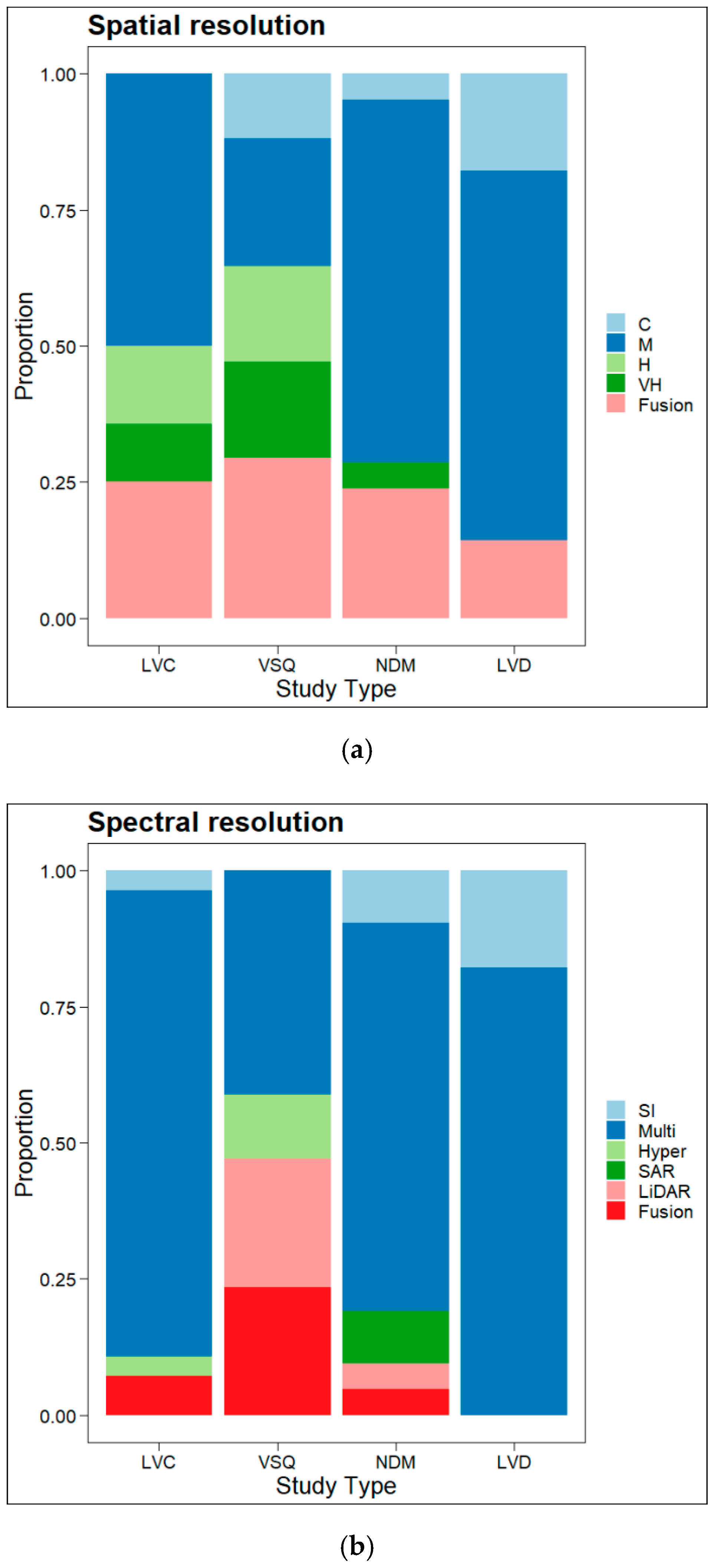
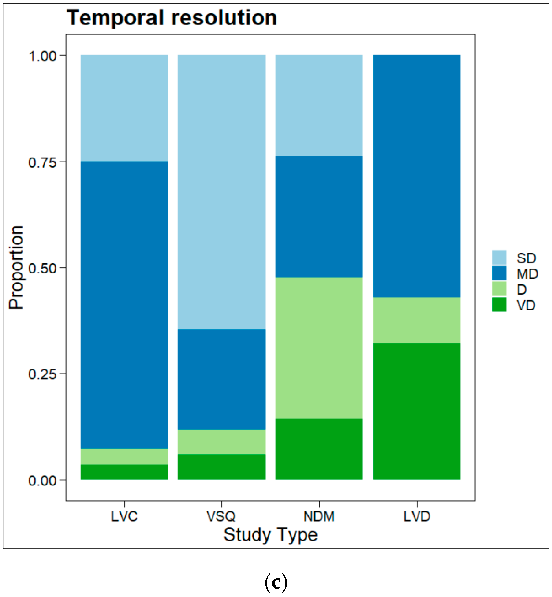
2.3.2. Remote Sensing Data Source

Various types of satellite data were used to monitor PAs (

Table 3. Remote sensing data used to monitor protected areas (PAs).

Remote Sensing Data	Pixel Size (m)	Study Type	Number of Studies	Examples
Coarse spatial resolution
MODIS (MOD09Q1, MOD10A1, MOD10A2, MOD13Q1, MOD15A2, MCD12Q2, MCD45A1, MYD14A2)	250, 500, 1000	LVC, VSQ, NDM, LVD	16	[31,32,33,34]
NOAA (AVHRR)	1000, 8000	LVC, VSQ	2	[35]
SPOT-Vegetation	1000	LVD	1	[36]
Moderate spatial resolution
Landsat (MSS, TM, ETM+, and OLI)	15, 30, 60, 80	LVC, VSQ, NDM, LVD	58	[37,38,39,40]
IRS (LISS III)	23.5	NDM, LVD	2	[41]
Resourcesat-2	23.5	NDM, LVD	2	[42]
EOS (ASTER)	15	LVC, VSQ, LVD	4	[43]
SPOT 2,4,5,6	5, 6, 10, 20	LVC, NDM, LVD	6	[44,45]
Sentinel-2	10	LVC, VSQ, LVD	5	[46]
High spatial resolution
IKONOS	4	LVC, LVD	2	[47]
RapidEye	5	VSQ, NDM, LVD	4	[48]
Hyperspectral
AVIRIS	10	LVC	1	[49]
HyMap	4	VSQ	1	[50]
APEX (Airborne Prism Experiment)	2, 3.35	LVC, VSQ	2	[51]
Very high spatial resolution
GeoEye-1	0.5	LVC, VSQ	2	[52]
WorldView-2	0.5, 2	LVC, VSQ, NDM	8	[53]
Airborne camera imagery (UCX, CIR orthophotos)	0.1524, 0.2, 0.305, 0.4, 0.5, 1	LVC, VSQ, NDM	6	[54,55]
SAR
Sentinel-1	10	NDM	1	[56]
PALSAR	30	VSQ, NDM	2	[57]
JERS-1	12	VSQ	1	[58]
TanDEM-X(TDX)	12	VSQ	2	[59]
LiDAR
ALS (Airborne laser scanning)	-	LVC, VSQ, NDM	7	[60,61,62]

). Moderate-resolution data were widely used (52%), and Landsat images were the most ubiquitous data (92.2%) due to their open access, appropriate spatial resolution, and long-term historical archive dating back to the 1970s. Apart from Landsat images, multispectral 10-m resolution Sentinel data, which have been available since 2015, were a common data type. Sentinel data have improved the classification accuracy, and their parameters are similar to those of Landsat data [30]. Since the emergence of commercial satellites, the spatial resolution gap between satellite images and aerial photographs has decreased; the proportions of high-resolution (e.g., RapidEye, Hymap, APEX) and very high-resolution (e.g., GeoEye-1, WorldView-2, LiDAR) data were 8% and 8.3%, respectively, in the reviewed studies. Very high spatial resolution satellite data, such as WorldView-2, provide sufficient detail for PA monitoring. A total of 8.6% of the studies used coarse-resolution data, and 87.5% of the studies used MODIS data for monitoring PAs with large extents, e.g., Etosha National Park in Namibia (22,270 km²), and KNP in South Africa (19,485 km²). In addition, studies that used a fusion of different resolution data comprised 23.1%.

Coarse data (i.e., MODIS) were most used in LVD and VSQ studies, and the MOD13Q1 product was used frequently (6 studies) since it provides two primary vegetation layers. Moderate and fusion data were used equally in studies of all topics, and high/very high-resolution data were mostly used to achieve accurate classification or perform quantification of vegetation structure (Figure 3a). For example, high-resolution imagery (aerial photography or satellite imagery such as WorldView-2) was preferred for detailed and accurate wetland mapping since it is difficult to discriminate between different wetland grass communities due to their composition, spatial heterogeneity, and limited spectral separability [63].

Most studies in our review used multispectral (or multiple VIs) data (68.6%), and the likely reason is that spectral information is important for identifying vegetation characteristics. Sirin et al. [45] compared land cover classifications of Meschera National Park obtained from Spot-5, Spot-6, Landsat-7, Landsat-8, and Sentinel-2 satellite data. The use of Sentinel-2 provided the highest accuracy (97.14%), whereas the Spot-6 (and Spot-7) data were inadequate due to the lack of a shortwave infrared (SWIR) band. This result indicated that spectral resolution is more important than spatial resolution for classifying peatlands. Various VIs have been established using remotely sensed data since there is a strong relationship between spectral reflectance and vegetation parameters. The NDVI was the most common VI in studies that used a single VI (9.2%); the reason is that the NDVI is regarded as a proxy of vegetation greenness. The majority of hyperspectral and LiDAR data were used in VSQ studies because these data types provide detailed information on the spectral and structural dynamics of vegetation. Although many studies have demonstrated that SAR sensors have the ability to penetrate vegetation canopies, SAR data were rarely used due to the interpretation complexity and relatively low spatial resolution.

Regarding temporal resolution, multidate data were used most frequently in our review (44.3%), followed by single-date data (28.4%), very dense data (14%), and dense data. Most of the VSQ studies used single-date data (64.7%), whereas LVC and LVD studies used predominantly multitemporal data, with proportions of 67.9% and 57.1%, respectively. This result shows that PA managers and scientists that are analyzing vegetation dynamics prefer multidate comparisons. Dense data were used almost equally for all study types, and very dense data (Landsat or MODIS time series products) were primarily used to detect trends in vegetation phenology but were used less in the other study types.

3. Current Approaches Used for Remote Sensing Monitoring of PAs

3.1. LULC and Vegetation Community Classification

The accurate classification of LULC and vegetation community types is important to maintain the ecological integrity and biodiversity of PAs; therefore, classification maps represent a baseline for the assessment of conservation management [64]. Many studies used traditional classification methods such as the maximum likelihood (ML) supervised algorithm or unsupervised ISODATA method to classify images to conduct PA change analysis in different landscapes (i.e., forests [20,65,66,67,68], wetlands [69,70], and glaciers [71,72]), differentiate savanna vegetation zones [73], or produce a mask for keystone species extraction [74]. Multiple endmember spectral mixture analysis (MESMA) was also used to distinguish vegetation species in a complex structure background. For example, Fairweather et al. [49] used MESMA to compare ASTER and AVIRIS imagery for the discrimination of soil, grass/forb, and sagebrush in Yellowstone National Park. The result showed that the use of readily available ASTER data with the MESMA method was most suitable for the accurate monitoring of large, semi-arid regions.

Machine learning classifiers are widely used in remote sensing due to the recent developments of advanced algorithms [75]. Compared with traditional parameterization methods, machine learning algorithms are more suitable for certain applications because they can handle large volumes of complex data over wide areas efficiently and accurately [76]. Commonly used machine learning classification methods in remote sensing include random forest (RF), support vector machine (SVM), decision tree (DT), and artificial neural network (ANN) methods [75].

RF was the most popular algorithm in our review (

Table 4. Machine learning algorithms used in our review.

Machine Learning Algorithms	Study Type	Number of Studies	Examples
RF	LVC, VSQ, NDM	20	[44,80]
SVM	LVC, NDM	7	[46]
ANN	LVC, NDM	5	[51]
DT	LVC	4	[63]

), because of the high accuracy and the ability to determine the relative importance of the predictor variables in the model [77]. For example, Chapman et al. [78] classified upland moorlands in the Peak District National Park in England into seven dominant land-cover classes using the RF algorithm and color and infrared aerial photographs. Herrero et al. [35] found out that the RF classifier was the best method for distinguishing African savannas in Chobe National Park in Botswana, which has a highly heterogeneous mixture of woody and herbaceous vegetation. Wendelberger et al. [53] observed that bi-seasonal data were more effective than single-season data to differentiate coastal plant communities in Everglades National Park. The authors combined bi-seasonal WorldView-2 multispectral data with LiDAR elevation data and used an RF classifier to map three mangrove and four adjacent plant communities, resulting in overall accuracy (OA) of 86%. Bassa et al. [79] compared RF and oblique random forest (oRF) algorithms for the classification of LULC classes in a highly heterogeneous PA using WorldView-2 image data. Both algorithms provided high classification accuracies (>80%), and although the oRF method resulted in higher accuracy (86.7%) than the RF method, there was no statistical difference between the two classifiers.

The ANN algorithm provides higher classification accuracy than other remote sensing image classification techniques, especially when the features are spatially complex, or the dataset has non-normal statistical distributions [63]. However, the large computational requirements limit its use compared to other better-known algorithms, such as RF and SVM [81]. For example, the ANN classifier was used for tree-species classification combined with high-resolution (3.35 m) APEX hyperspectral images (the bands are in the visible and near-infrared (VNIR) spectral region) for the classification of Karkonoski National Park in Poland; a median OA of 87% [51] was obtained.

The extent and characteristics of the landscape matrix are important factors affecting the accuracy of LULC classification and vegetation community mapping, and there is no single best classifier that can handle all conditions because the ground features may differ in different ecosystems. Many comparative studies were conducted to assess multiple classifiers. For example, Szantoi et al. [63] applied traditional (i.e., the ML method) and machine learning classifiers (i.e., the DT and ANN methods) for the mapping of heterogeneous wetland plant communities in Everglades National Park using airborne high spatial resolution data. NDVI and texture features were obtained, and the results demonstrated that the ANN classification accuracy was the highest (82.04%) under several conditions, and the texture features significantly improved the classification accuracy. Rapinel et al. [46] compared Sentinel-2 time-series and single-date datasets using SVM and RF classifiers for discriminating plant communities in wet grasslands. The results showed that the date had a greater influence than the spectral band on the classification accuracy; the SVM classifier slightly outperformed the RF classifier (Δ = 0.07 in OA). Rather than comparing the accuracy of machine learning algorithms, Bai et al. [31] input the LULC classification results of three different classifiers (ML, ANN, and SVM) into an ensemble classifier for the classification of the Mount Wutai World Heritage Area.

Open-access platforms that provide global-scale earth observation data storage and a user-friendly interface have seen increased use in remote sensing research since they have high processing capacity (e.g., Google Earth Engine (GEE) [82]) [35,64,80]. Tsai et al. [64] used the cloud-based GEE platform and different Landsat composite images to compare the performance of the RF and DT algorithms for LULC and vegetation classification in the Fanjingshan National Nature Reserve. The classification product generated using the RF classifier with seasonal composite images yielded the most stable and most consistent high-accuracy maps (with the highest accuracy of 77%) of the mountainous forested areas that are often obscured by clouds. Shores et al. [74] demonstrated that temporal information is more important than spatial information for mapping huckleberry ecosystems in Glacier National Park. The study exploited the seasonal leaf color changes using 1-m resolution National Agricultural Imagery Program (NAIP) imagery and multitemporal Landsat imagery; the RF classifier provided high accuracy.

Object-based image analysis (OBIA) methods incorporate spatial neighborhood properties into the classification process, thus minimizing sensor limitations and producing a more accurate representation of landscape patterns than pixel-based methods [43]. Recently, OBIA was widely used in combination with machine learning classifiers to extract forest information, such as DT [83], SVM [84,85], and RF [60]. In these studies, both spectral and textural features were used to improve the accuracy of OBIA classification. For example, Xofis and Poirazidis [83] used OBIA and classification and regression trees (CART) approaches to map land cover change in the Dadia-Lefkimi-Soufli Forest National Park. The OA of the mapping products increased from 73% for single-use very high resolution (VHR) images (GeoEye) to 89% for the combination of VHR images and Landsat-5 images. Gonzalez et al. [60] combined LiDAR with high-resolution spectral data and used OBIA and an RF classifier for landcover classification in the BFNP; high accuracy (with an OA of 86.6%) was obtained in the absence of field survey data. Although shadows are often treated as unwanted noise and are masked in most remote sensing research, they can be useful in OBIA classification. For example, Carter and van Leeuwen [54] developed an automatical mapping tool for the detection of individual saguaros using shadow signatures and fine-resolution digital aerial imagery.

3.2. Vegetation Structure Quantification

Forest structural and functional variables, such as tree height (TH), canopy closure (CC), basal area (BA), diameter at breast height (DBH), stand volume (SV), aboveground biomass (AGB), and leaf area index (LAI), are considered reliable and repeatable indicators for understanding the health and function of forest ecosystems and their response to global climate change. Spatial information on forest structure is a crucial element of forest inventory and is used as a proxy of carbon stock and fluxes [86], and also provides a baseline for the sustainable and sound management of PAs. Optical remote sensing data are widely used to derive vegetation structure characteristics using physically based radiation transfer models (RTMs) or empirical statistical models [87]. Atzberger et al. [50] illustrated the disadvantages and advantages of the physical and empirical models using the airborne hyperspectral HyMap instrument for estimating LAI. A comparative analysis was conducted among four different retrieval methods (two RTM inversion methods and two statistical modeling methods) for mapping Mediterranean grasslands in Majella National Park, Italy.

Empirical regression models were commonly used in the reviewed studies to model the relationship between the in-situ measurements of vegetation structure variables and spectral VIs [88] or spectral data combined with textural features [48,52]. For example, Czerwinski et al. [88] used an empirical statistical method based on a VI derived from Landsat 5 TM image time series and field measurements. Forest changes were mapped in Gatineau Park, Québec, and it was found that the Tasseled Cap Wetness (TCW) was the most robust index. Dube et al. [38] used Landsat-8 derived VIs and RF regression to assess the spatiotemporal seasonal LAI dynamics (dry and wet seasons) as a proxy for rangeland conditions and productivity in KNP.

Texture information is an increasingly important aspect of remotely sensed data analysis, as mentioned above. Gomes and Maillard [48] modeled the regeneration process of Cerrado vegetation based on multiple regression analysis. A RapidEye image mosaic and textural features derived from the grey-level co-occurrence matrix (GLCM) were used to estimate the age, CC, and TH of the vegetation. Van Coillie et al. [52] modeled critical forest structural attributes, such as the crown diameter (CD), SV, and TH, using a GeoEye-1 image within an OBIA framework and derived the composition of the Acacia tortilis population in Bou-Hedma National Park in South Tunisia. The population of A. tortilis was characterized by an irregular structure, and it was confirmed that the species had suffered from regressive population dynamics. Fatehi et al. [87] estimated the forest structural attributes, including CC, BA, and SV, in heterogeneous alpine ecosystems in the Swiss National Park using APEX data in combination with simple and stepwise multiple regression models.

MODIS vegetation products have been widely used to retrieve vegetation composition. Tsalyuk et al. [32] analyzed time-series data of four MODIS vegetation products (NDVI, EVI, LAI, and the fraction of photosynthetically active radiation (FPAR)) in Etosha National Park. Multiyear partial least-squares regression (PLSR) models were created to predict the density, cover, and biomass of the dominant savanna vegetation forms (grass, shrubs, and trees) based on extensive field data. The results showed that the EVI produced the best model for grass and shrub cover, and NDVI was the best predictor of tree density and cover, whereas FPAR was the best predictor of biomass. Vaz et al. [89] used the EVI in the MOD13Q1 product for describing seasonal vegetation changes in Peneda-Gerês National Park, Portugal. Ibrahim et al. [90] developed a remote sensing model that included linear, logarithmic, and polynomial regressions to retrieve woody cover in African savanna based on the NDVI and soil-adjusted vegetation index (SAVI) derived from MODIS data and field data from 28 sites in KNP. A comparison of the results of several products indicated that the LiDAR/SAR data were more accurate for the estimation of woody cover than the other data.

Many uncertainties exist when field measurements of the ecosystem characteristics and optical remote sensing data are used for the estimation of forest structural parameters [91]. In contrast, the detail and accuracy of the three-dimensional (3D) representation of the forest structure at multiple scales have significantly improved with the use of airborne and spaceborne stereo viewing capability, interferometric SAR, and LiDAR. SAR imagery is suitable for wetland monitoring since the radar backscatter signal is highly sensitive to the wetland biophysical parameters. Lucas et al. [58] retrieved comprehensive information on the biophysical properties of mangroves (forest age, CC, TH, and AGB) from spaceborne optical and SAR data to obtain a better understanding of the vegetation dynamics in a managed setting in the Matang Mangrove Forest Reserve (MMFR). Combining optical images with SAR images, Huang et al. [92] developed a set of models, including curve estimation, linear regression with multiple variables, and back-propagation neural network (BPNN) modeling, for estimating AGB in Xixi National Wetland Park in Hangzhou in China. The results showed that the SAR models generally had better accuracy than the optical models, and the BPNN models achieved the highest accuracy among all models.

LiDAR has higher spatial resolution than optical and radar data and is a powerful technology for measuring and mapping AGB stocks and other forest structure parameters, despite the expensive acquisition cost [90,93]. For example, LiDAR datasets have been used to verify physically based models to obtain AGB [94] and have been integrated with conventional allometric equations to simplify the quantification [95] and monitoring [59] of AGB and assess the temporal and spatial patterns of treefall [61] or deadwood [96] in PAs. Fernandez-Landa et al. [95] evaluated new methodologies to obtain spatially explicit LiDAR biomass inventories based on local and general plot-aggregate allometry and confirmed that the general plot-aggregate methodology was an easier approach to obtain BA through LiDAR top-of-canopy height data since BA was the only field measurement required. Treefall datasets were identified and mapped using canopy height and shape obtained from multiyear LiDAR data using a crown segmentation approach. Environmental data, elephant density, and fire regime maps were used as potentially explanatory variables to describe treefall rates quantitatively in KNP using an RF model [61].

3.3. Natural Disturbance Monitoring

Natural disturbances, such as wildfire, insects, diseases, windthrow, and flooding, are recognized as major drivers of global change in terrestrial ecosystems. Therefore, the accurate monitoring of the disturbance type, size, and impact over large areas is becoming increasingly important [57]. Remote sensing has been used extensively for forest disturbance owing to its long-term data archive and near real-time ability to detect changes.

3.3.1. Wildfire Disturbances

Wildfire is one of the greatest challenges in PA management due to its impact on the environment, i.e., greenhouse gas emissions, acceleration of ecosystem degradation, and wildlife extinction. Exaggerated by global climate change, devastating wildfires have become more frequent in recent years and will intensify in the future [97]. An analysis of fire disturbances can provide additional information for PA management. Munyati and Sinthumule [98] used panchromatic aerial photographs and SPOT images for detecting fire and elephant damage that caused changes in woody cover in KNP. Satish and Reddy [41] compared the fire frequency between the core area and buffer zone of Silent Valley National Park and correlated fire frequency with the topography, climate, and road and settlement density from 1973 to 2014. It was found that fire prevention measures in the national park reduced the occurrence of fires in the core area, demonstrating the effectiveness of park management. On the other hand, proponents of the view that fire harms biodiversity and threatens cultural heritage are in favor of fire suppression, which may aggravate social conflicts and cause high fire rates. Batista et al. [99] compared the fire regimes of areas in Canastra National Park in southeast Brazil managed with and without fire suppression using 16-year Landsat imagery. The monitoring of fire disturbances in PAs using remote sensing techniques has mainly focused on pre-fire prediction and post-fire evaluation of fire regimes, as described by the fire extent, intensity, and frequency.

Preventive action is effective for wildfire management. GIS and remote sensing data were used to create fire susceptibility (or vulnerability) maps in several PAs [100,101]. The methods and techniques for susceptibility mapping can be classified into three groups: probabilistic, statistical, and machine learning methods [101,102]. Probabilistic methods simulate and predict the potential behavior of forest fires using mathematical functions and equations. The most important tasks are the selection and weights of the variables used in the equations. Amalina et al. [103] used land cover, VI, moisture index, surface temperature, and the distance from roads, rivers, settlements, paddy fields, dryland farms, and plantations as variables and conducted an analysis based on the concept of the fire triangle. The authors compared two equations; one equation had a high weight (90%) for the human factor, and the other equation had a 90% weight for natural factors. The results showed that one of the natural factors (availability of fuel material) had a significant influence on triggering the occurrence of forest fires caused by human activity in the Way Kambas National Park, especially in the dry seasons. Mukti et al. [100] used similar factors (landcover, spectral index, and terrain data) and an empirical equation to evaluate the influence of fires in Alas Purwo National Park. Gigovic et al. [101] synthesized fire inventory data derived from satellite images, a historic fire database, and field surveys to improve the accuracy of fire susceptibility evaluations. The authors compared the results of forest fire susceptibility maps obtained from supervised and versatile machine learning algorithms (SVM and RF) and an ensemble model in Tara National Park, Serbia. The results demonstrated that the ensemble model using the Bayesian average had the best performance, followed by the RF algorithm.

It is important to understand the historical fire regimes of PAs to predict fire trends [104]. MODIS fire products were utilized for assessing fire trends at large scales. For example, All et al. [105] used MODIS fire products (MYD14A2 and MCD45A1) for analyzing the patterns in fire occurrence, seasonality, and spatial distribution from 2002 to 2014 and assessed the relationships between temperature, precipitation, and fire activity in Huascarán National Park. Burned area extraction is a common task in fire regime studies, and fine spatial resolution data (e.g., Landsat or Sentinel) enable the accurate delineation of small and patchy fires, which cannot be detected by MODIS. Different methods were proposed to enhance and detect burned areas and minimize spectral confusion [106]. Spectral indices derived from Landsat images were frequently used to detect land cover changes by comparing the spectral characteristics before and after fire occurrence [39,107]. Costa dos Santos et al. [39] evaluated the potential of using a multitemporal NDVI and NBR analysis to extract the fire extent. The limitations included the presence of clouds and topographic shadows in the images and the revision time of the satellite data. Kato et al. [107] addressed these problems by using composite time-series Landsat images and the GEE platform to mitigate cloud and shadow effects and quantified the trends in fire size and frequency in Wood Buffalo National Park.

Furthermore, visual interpretation methods are often better suited for the detection and delineation of burned areas than automatic procedures, which often confuse burned areas with other elements of the landscape with similar spectral patterns, such as water, cloud shadows, or topographical features [41,99]. Daldegan et al. [108] obtained low accuracy for a supervised classification approach for burned area mapping in the Serra Tombador Natural Reserve and its surroundings using several Landsat TM images acquired in the dry season between 2001 and 2010. The authors adopted a post-classification method using expert visual interpretation to determine the spatial patterns of fire recurrence in different land cover classes.

The spatial distribution of vegetation recovery dynamics after fire disturbances is essential for developing management measures that promote the transformation and ecological restoration of burned areas [109]. Fang et al. [110] mapped the LAI and tree sapling abundance (TSA) after a wildfire in the Huzhong National Natural Reserve using Landsat and WorldView-2 imagery and an RF model to assess the relative importance and causal mechanisms of the spatial controls and their effects on tree sapling recovery; it was concluded that mitigating wildfire severity and size may increase forest resilience to wildfire damage. However, large areas of dense regrowth after a fire can pose a significant fire risk to the PA, which is of particular concern to PA managers both in the short- and long-term. Gordon et al. [62] used airborne LiDAR data for measuring post-fire mid-story vegetation regrowth and investigated the effect of fire severity on the regrowth amount and spatial pattern following the wildfire using linear mixed-effects models in Warrumbungle National Park, Australia.

3.3.2. Flood Disturbances

Flooding is considered the most damaging natural hazard in the rainy season and has adversely affected biodiversity and ecosystem functions in some PAs. Diaz-Delgado et al. [111] presented a semi-automatic procedure to discriminate seasonally flooded areas in the shallow temporary marshes of Doñana National Park in Spain. The historical spatial and temporal patterns of flooding events and the hydroperiods were reconstructed using radiometrically normalized long time-series Landsat images (1974–2014). Ghosh et al. [112] used Landsat-8 OLI for water extent mapping and SARAL/AltiKa for water level mapping in Kaziranga National Park during one of the most devastating floods of 2016. Because of the low availability of cloud-free optical data sets during the monsoon season, SAR data were preferred for detecting inundated areas and provided reliable information during a flood event due to their all-weather, all-day, and near real-time capabilities and the ability to penetrate vegetation canopies. For example, Borah et al. [56] analyzed the spatiotemporal flood inundation in Kaziranga National Park and surroundings using C-band Sentinel-1 data and unsupervised classification during the monsoon season of 2017.

3.3.3. Forest Insect Disturbances

The central European forests are less threatened by abiotic natural hazards, such as wildfire and floods, but European spruce bark beetle infestations pose a serious risk to forest health [113,114]. Numerous remote sensing techniques have been used to monitor and assess bark beetle-caused tree mortality, the impact of defoliators, and tree declines in forest ecosystems of the BFNP in Germany, including the use of multitemporal Landsat/SPOT imagery [44,113], aerial color-infrared photography [55], high-resolution satellite imagery [33], and SAR imagery [57].

Latifi et al. [44] combined multidate Landsat and SPOT data to map the spatial characteristics of bark beetle infestations; an OA of 80% was achieved using the RF method and the original reflectance data. Latifi et al. [113] subsequently refined this approach by including digital elevation models and using OBIA with RF to map the forest mortality classes over 11 years in the BFNP. A window-independent context segmentation (WICS) of the color-infrared aerial photos was proposed for the yearly monitoring of deadwood areas in the BFNP; a time-effective and accurate classification was obtained [55].

The remote sensing community has become increasingly interested in fusing spatial and temporal features of different image datasets and generating composite data with fine resolution. Latifi et al. [33] applied a flexible spatiotemporal data fusion (FSDAF) approach for blending MODIS and RapidEye reflectance and created eight-day composites of synthetic RapidEye-like NDVI data for identifying Norway spruce mortality caused by bark beetles. Stych et al. [115] evaluated the usefulness of very high spatial resolution images (WorldView-2) and moderate spatial resolution images (Landsat 8 OLI) to identify forests infested by bark beetle outbreaks from satellite data using SVM and ANN in Sumava National Park. The SVM was considered the best method and achieved the highest OA (86%) with WorldView-2 data. Tanase et al. [57] used L-band PALSAR images and a simple mapping approach based on thresholds to detect insect outbreaks and windthrow events. The backscatter value of the SAR data was used to delineate areas affected by insect outbreaks in the early stage; however, the use of backscatter change values alone was limited because it could be confused with other factors (e.g., fire, logging); therefore, ancillary information might be needed to determine the disturbance agent.

3.4. LULC and Vegetation Dynamic Analysis

Free access to remote sensing time-series images has allowed for novel methods of mapping and monitoring of dynamic phenomena, thereby increasing the number of studies of LULC change detection and monitoring the status of natural vegetation in PAs. Dynamic information on the vegetation status in and around PAs is crucial to assess management performance because it supports the assessment of habitat suitability, biodiversity, and vegetation productivity [36].

3.4.1. Spatial and Temporal LULC Change Detection

LULC dynamics of PAs have become a key issue in many disciplines, such as forestry, agriculture, environmental science, geology, and hydrology. Many researchers have evaluated the effectiveness of PAs using multiperiod remote sensing data, such as describing LULC changes in PAs, comparing LULC changes inside and outside of PAs. In many cases, areas outside PAs are often heavily influenced by human activities [116,117], and the results of studies have provided suggestions for PA management. Within the past three decades, numerous change detection techniques using satellite imagery have been developed and applied, including post-classification comparison (PCC) [84,116], principal component analysis (PCA) [118], and VI differencing [30].

PCC was most frequently used in PA monitoring, especially in developing countries due to the constraints on data availability and processing ability [42,84,119]. PCC is considered an efficient approach for the detection of large areas of change because multiperiod images are compared, and data normalization is not required since images of different dates are classified separately. This approach minimizes the difficulties in change detection associated with the analysis of images acquired at different times of the year, or from different sensors. For example, Rui Mucova et al. [84] compared forest loss in Quirimbas National Park in Africa using five classified Landsat TM images from 1979 to 2017 and proposed mitigation and management suggestions. Some studies compared landscape metrics and LULC dynamics before and after the establishment of PAs to analyze the driving forces of disturbance [116,120], demonstrate the effectiveness of the establishment and management of PAs [121], or conduct conservation planning [70,119]. For example, Vorovencii [67] used several classified Landsat satellite images and six landscape metrics to quantify forest fragmentation in the pre- (1986–2002) and post-establishment (2002–2016) periods, inside and around Apuseni Natural Park, Romania. The results showed that forests have suffered from continuous loss due to fragmentation.

The reliability of PCC depends on the classification accuracy of the individual images because the error of the comparison images equals approximately the product of the classification errors of the individual images. However, a classification that is based solely on spectral information is often not sufficiently accurate and is unable to describe LULC change in the research area accurately. Therefore, machine learning algorithms, coupled with various predictors, were used to improve the accuracy (as described in Section 3.1.). A major challenge in PCC is the acquisition of reliable training data for historical images; commonly used methods to obtain training points are the use of high-resolution spaceborne data (e.g., WorldView-1 or Google Earth images [37,119]), combined with field survey data. Scharsich et al. [117] did not have field data for a study in Matobo National Park, Zimbabwe and proposed a change-vector analysis to find pixels that remained unchanged over time as training points for the RF classifier. Another disadvantage of PCCs is that gradual and subtle ecosystem changes cannot be detected. There are many advanced algorithms based on Landsat imagery capable of capturing both gradual and abrupt changes, such as Landsat-based detection of Trends in Disturbance and Recovery (LandTrender), Vegetation Change Tracker (VCT), and Continuous Change Detection and Classification (CCDC) [122]. However, these algorithms have not been used for PA monitoring in the studies we reviewed.

Some studies focused on the prediction of LULC change based on PCC. Bozkaya et al. [123] evaluated the capability of a stochastic Markov (St-Markov) model and cellular automata Markov (CA-Markov) model for simulating LULC change in the Igneada PA. The results showed that the CA-Markov model provided more reliable information than the St-Markov model. Roy and Rathore [124] generated future LULC trends using the CA-Markov and agent-based LULC-SaarS models for management planning in Corbett National Park in India. Some researchers used regression modeling to investigate the relationship between LULC change and the driving factors to predict future trends. For example, Htun et al. [20] examined the factors influencing deforestation and forest degradation changes over time in the Popa Mountain Park in Myanmar. Multinomial logistic regression was used; the forest cover change maps derived from Landsat images were the dependent variables, and spatial and biophysical factors (elevation, slope, aspect, distance from villages, roads, and the park’s circular road) were the independent variables. The relationships between land cover change and its driving factors can be very complex and are often non-linear. Therefore, Khoi and Murayama [125] predicted areas vulnerable to forest conversion in the Tam Dao National Park using remote sensing data and a model consisting of a multilayer perceptron neural network and a Markov chain (MLPNN-M) model.

Several studies have highlighted the importance of participatory approaches, which provide a narrative perspective grounded in the experiences and concerns of residents, to understand the relationships between the driving forces and the patterns of LULC change and target management efforts [47,65]. For example, Sassen et al. [65] used a combination of satellite image analyses and surveys of the local inhabitants, including village meetings with semi-structured discussions to understand the drivers of forest cover change in Mount Elgon National Park from 1973 to 2009. Garrard et al. [47] evaluated LULC changes that occurred during 1992–2011 in Sagarmatha National Park by combining multitemporal satellite imagery and sociological information gathered from local interviews and workshops to determine the underlying driving processes.

3.4.2. Estimation of Vegetation Health Dynamics

Long-term trends in vegetation loss (browning) or improvement (greening) are important for assessing conservation strategy implementation in PAs. Vegetation health dynamics can be mapped through continuous monitoring of vegetation phenology using time-series remote sensing data to identify the dominant spatiotemporal patterns occurring in PAs. VI trend analysis is a common method to characterize the changes in vegetation health. The most commonly used VI is NDVI, which is widely used in studies of vegetation health and productivity and can detect greening trends over time by month or by season. For example, Herrero et al. [35] conducted an NDVI analysis based on monthly AVHRR NDVI data to determine the long-term trends of the landscape in Chobe National Park in Botswana during 1982–2011. Davies et al. [126] determined the spatial and temporal extent of historical changes in vegetation patterns in the Phnom Kulen National Park by comparing NDVI and EVI obtained from two calibration methods (relative radiometric normalization and RTM) that were used to convert Landsat L1 level images to surface reflectance. The EVI was more resilient to residual atmospheric effects than the NDVI. In addition, a normalized difference moisture index (NDMI) time series was used to quantify clearcutting events and early forest recovery times in the mangrove ecosystem of the MMFR using annual Landsat time series [40]. Van Dongen et al. [127] used the cumulative sum of the Landsat time-series i35 index in combination with field-based measurements and obtained a comprehensive change image that showed the impact of destocking on the vegetation cover of Dirk Hartog Island.

Since natural hazards, such as wildfires or persistent drought, often change the appearance of vegetation, thereby affecting the statistical distribution, nonparametric Mann–Kendall and Theil–Sen tests were used to determine the significance of the greening trends obtained from MODIS products [128] and Landsat-derived NDVI time-series data [129,130]. Zurita-Milla et al. [36] used a nonparametric unsupervised self-organizing map and Sammon’s projection method to create 13 years of ten-day NDVI composites from SPOT-Vegetation NDVI time-series data to characterize the dominant phenological states of KNP. Senf et al. [131] integrated the advantages of the fine temporal resolution of MODIS and the medium spatial resolution of Landsat images to develop a new Bayesian hierarchical modeling approach for estimating the spatial and temporal variations in the spring phenology of broad-leaved forests in the BFNP using all available Landsat time-series images.

Additionally, the Breaks for Additive Season and Trend (BFAST) algorithm is highly resilient to noise and missing data (i.e., low data availability or cloud cover) and can produce sub-annual information on vegetation trends; MODIS data are often used as the input. Murillo-Sandoval et al. [132] applied BFAST to the MODIS-based multi-angle implementation of atmospheric correction and used all available Landsat images to monitor short-term forest disturbances and long-term trends in the cloud-prone Picachos National Park in the Colombian Andes during 2001–2015. Murillo-Sandoval et al. [133] used the BFAST Monitor algorithm and dense Landsat time-series data for detecting sub-annual forest cover disturbances and integrated an RF classifier for characterizing the drivers of the conversion to pasture, agriculture, and non-stand replacing disturbance (i.e., thinning). The limitations of the BFAST algorithm included an inability to identify multiple, sequential disturbances in a given pixel over the time-series and determine the causal linkages between specific drivers.

Our understanding of how climate drives vegetation dynamics has evolved rapidly with the help of remote sensing datasets and statistical analyses. Remote sensing data, in conjunction with weather data, have been used to determine the response of PA landscapes to climate change. Satellite observations from coarse-resolution sensors (i.e., MODIS and AVHRR) have been widely used to study the impacts of climate anomalies on vegetation phenology. For example, Norman et al. [34] used MODIS NDVI time-series data and a regression model to ascertain the environmental gradients (i.e., topography, forest cover type, disturbances, and temperature and precipitation within and between seasons) of the variations in spring and autumn timing from 2000 to 2015 in Great Smoky Mountains National Park, USA. Wallace et al. [134] created a suite of Climate Landscape Response phenometrics based on the strong correlation between the precipitation data of the Parameter-Elevation Regressions on Independent Slopes Model (PRISM) and MODIS NDVI composites using a simple linear regression model to predict the greenness of invasive buffelgrass in the dryland areas of Saguaro National Park.

Some studies have focused on the relationship between snow phenology and vegetation change and have found that the vegetation greening timing and snow cover duration had important influences on the ecological functions. MODIS time series products can be used to monitor vegetation and snow phenology. For example, O’Leary et al. [135] used MODIS data (MCD12Q2) to assess the influence of snowmelt timing and elevation on five phenology metrics (green-up, maximum greenness, senescence, dormancy, and growing season length) in Crater Lake National Park from 2001 to 2012. Swanson [128] combined MODIS NDVI composites (eMODIS), MODIS Terra Snow Cover Daily data (MOD10A1), and long-term weather records and observed that the average snow-off and green-up dates occurred about 6 days earlier over 80 years. In contrast, a slight increase in persistent snow cover was observed in Karakoram National Park during 2001–2010 from MODIS snow data (MOD10A2); enhanced glacier preservation occurred in the ablation areas due to longer-lasting snow cover and stronger accumulation at higher altitudes [72].

4. Challenges and Future Work

The development of remote sensing instruments and analysis methods has provided an opportunity for advanced studies on PA monitoring to provide meaningful insights. Further research is expected to focus on the following topics.

4.1. Development of Remote Sensing Frameworks for Local PA Monitoring Worldwide

Remote sensing monitoring at the global scale is insufficient to provide details on the protection level of and threats to specific PAs. The use of remote sensing for PA monitoring has substantially increased; however, some areas are still lacking remote sensing monitoring, particularly developing countries (such as Africa) where ground-truth data are sparse. Only three studies were found in Australia due to the limited criteria and database used in our research, which excluded plot-based studies [136]. Regular monitoring of entire PAs relies largely on field monitoring by PA management agencies [137] or consists of participatory monitoring and evaluation [138]. Nevertheless, expanding the search across multiple databases [23], such as Google Scholar and Scopus, will reduce omissions of studies. There is a need to leverage PA monitoring worldwide, and the remote sensing framework should be extended to most of the PAs to determine the level of protection. The challenge is to integrate appropriate data and methodologies best suited for the local ecosystems into an efficient, transferable, and continuous monitoring framework [31,32,54,80,139], which provides a baseline for evaluating the effectiveness of PA management practices and conservation strategies to achieve international conservation goals.

4.2. Comprehensive Utilization of Multisource Remote Sensing Data

Free and open-source remote sensing data (especially Landsat and Sentinel) remain an important data source for PA monitoring. Higher spatial resolution is needed [68] because it affects the accuracy of the land-use classification and the identification of sensitive species, especially in small areas with high spatial heterogeneity [32,63]. SAR imagery is suitable for wetland monitoring [58] and flood mapping [56], and multitemporal LiDAR data can be extensively used to quantify vegetation structural dynamics [59,62]. The synergy of multisource data, such as multispatial data [85] and active and passive [60] data, can compensate for the shortages of single-date data and improve the accuracy of feature extraction, especially in remote and extensive PAs. As mentioned above, in the reviewed studies, temporal information had a greater influence than spatial [74] and spectral [46] information for determining rapid or seasonal changes; therefore, we should make use of dense data in future studies [46,57]. In addition, the integration of multisource data can be facilitated by freely available cloud platforms, such as GEE (https://earthengine.google.com/), the Application for Extracting and Exploring Analysis Ready Samples (AppEEARS) (https://lpdaacsvc.cr.usgs.gov/appeears/), the Sentinel EO browser (https://apps.sentinel-hub.com/eo-browser), the System For Earth Observations, Data Access, Processing and Analysis For Land Monitoring (SEPAL) (https://sepal.io/process), and free analytical tools such as eHabitat and IMPACT, which are designed specifically for PAs and have low technical barriers to the extraction of useful information from remote sensing datasets [139]. Additionally, imagery from low-cost and flexible unmanned aerial vehicles with very high spatial resolution can be valuable for retrieving or validating land cover types and vegetation parameters [30,58,85] from moderate-resolution or SAR data. These data can be uploaded to platforms such as OpenAerialMap (https://map.openaerialmap.org/) for public and broad use [58].

4.3. Improving Methods to Assess the Details of PA Dynamics

Significant advances in remote sensing technologies suitable for PA monitoring have been made in the last decade. For example, classification research has changed from using a single classifier to the integration of different classifiers [31,83] and the comparative study of multiple machine learning classifiers [46,63,64]. Machine learning algorithms, such as RF and SVM, have become popularized recently; however, the selection and combination of different variables [37,38,60,74,110] (e.g., spectral bands, VIs, texture features, and topographic attributes) in the model to avoid multicollinearity and to enhance the accuracy of the extracted information remain challenging. Deep-learning algorithms may be helpful for processing high-dimensional hyperspectral remote sensing data [51]. Furthermore, advanced change detection algorithms are rarely used for individual PA analysis [129,133], although they can capture details of landscape change and can determine the drivers of specific events from dense time-series data. Advanced algorithms such as LandTrender [140], VCT [141], or CCDC [142], which have been implemented in GEE [143], should be used more extensively to determine subtle changes and even obtain near real-time information for identifying potential risks at the early stage in future studies.

Appropriate methods and algorithms were chosen for different ecosystems and objectives in our review. PCC was considered efficient for change detection because of its simplicity and intuitiveness, but there are limitations due to the lack of reliable training data for historical images [37,119]. In addition, identifying and collecting sufficient ground training samples remains a significant challenge, especially in PAs dominated by extensive forests [46,51,64]. The change-vector analysis [117], which was mentioned in Section 3.4.1, is not a suitable method when built-up areas are present in intact forest. The studies in our review mostly used very high resolution imagery as reference data for selecting training and validation samples; however, PA managers are familiar with local conditions, perform regular ground-based monitoring, and are concerned about the dynamics of PAs under different pressures [84]. The following measures can be considered to address this issue: integrating very high resolution data with the trajectory information from time-series Landsat archives and expert knowledge of PA managers and local residents; developing stable ground-based sampling networks [144] focused on ecologically vulnerable areas and performing consistent monitoring; and encouraging visitors to participate in science observation plans [134] in the future.

4.4. Discovering the Driving Forces and Providing Measures for PA Management

Quantitative information on the trends in LULC [80,118], vegetation health [30], forest fragmentation pattern [67], and the characteristics of disturbances [41,99,107] in PAs or a comparison between areas with different management strategies allows for estimating the efficiency of the PA management strategy. For example, a decrease in the vegetated area and an increase in human settlements indicates the failure of conservation efforts [84], whereas an increasing trend of forest cover and a decrease in agricultural land use suggests that the PA is well protected [117]. A major challenge is how to provide valuable insights into site-specific PA management through the interpretation of remote sensing images rather than just describe the symptoms [42]. Remote sensing has the potential to identify the complex drivers of change in human-nature coupled systems, which is generally induced by human activities (including human settlements [66], urbanization [31], excessive tourism [35], mining [85], logging [67], agriculture expansion [37], grazing [127], and hunting [124]) and natural disturbances (including climate variabilities such as droughts [101] and sea-level rise [53], as well as species invasions [118] and megafauna roaming [61,98]). The analysis of remote sensing data alone has limits for discovering accurate and reliable information on the driving forces that threaten ecosystems and for proposing countermeasures for PAs. A broader interdisciplinary approach is suggested with the help of essential information that covers both natural and socioeconomic dynamics, such as climate data [105,130,134] (e.g., precipitation, temperature), population and dispersal pattern of fauna [85,96], resident population [20,37], GDP [130], agricultural calendar [118], and government strategies [117,118].

Some of these data can be obtained from conservation authorities [118], field-based biodiversity surveys [85], or literature analyses [120]. In contrast, many socioeconomic data (such as population census and GDP) are often based on administrative districts, and data at the local level are unavailable inside the PA boundary. Thus, there is a need to conduct local observations. Social studies can be integrated using interviews with the local population [47,84] or semi-structured questionnaires [65,120], which provide information on the experiences and concerns of residents and PA managers that is crucial in understanding the linkages between the driving forces and the outcomes derived from remote sensing observations [47]. The management effort of PAs is another challenge and should focus on three topics: implementing and enforcing laws (e.g., prohibiting destructive activities [67] such as illegal mining and deforestation), communicating and cooperating with the local community (e.g., awareness campaigns [67], community empowerment [68]), and providing regional planning suggestions for PA management (e.g., delineation of hierarchical functional zones [120], identifying priority areas for protection actions [108], creating ecological corridors [84], establishing more botanical reserves [119], reforestation [30], and prescribed burning practices [99]).

5. Conclusions

We conducted a systematic review of the literature on remote sensing monitoring of individual PAs and found that this topic has become increasingly important worldwide, and specific methods and sensors are particularly useful for certain research objectives. It is necessary to improve the integration of remote sensing technology with PA management efforts and use these methods actively for biodiversity conservation. We identified several challenges in the current stage. Future studies should focus on utilizing multisource data, advanced technologies, and field-based investigation to develop a continuous monitoring framework that integrates multi-interdisciplinary knowledge, especially local knowledge, to identify the driving forces of change and provide comprehensive information for PA management and decision-making. The use of remote sensing as an efficient tool for evaluating the progress of implementing international conservation commitments and achieving sustainable development of PAs is highly promising.

References

1. Protected Areas: About. Available online: https://www.iucn.org/theme/protected-areas/about (accessed on 18 March 2020).
2. Protected Areas Map of the World. Available online: https://www.protectedplanet.net (accessed on 18 March 2020).
3. Protected Planet Live Report 2020. Available online: https://livereport.protectedplanet.net (accessed on 18 March 2020).
4. Neugarten, R.A.; Moull, K.; Martinez, N.A.; Andriamaro, L.; Bernard, C.; Bonham, C.; Cano, C.A.; Ceotto, P.; Cutter, P.; Farrell, T.A.; et al. Trends in protected area representation of biodiversity and ecosystem services in five tropical countries. Ecosyst. Serv. 2020, 42, 101078. [Google Scholar] [CrossRef]
5. Diniz, M.F.; Cushman, S.A.; Machado, R.B.; Júnior, P.D.M. Landscape connectivity modeling from the perspective of animal dispersal. Landsc. Ecol. 2019, 35, 41–58. [Google Scholar] [CrossRef]
6. Coad, L.; Leverington, F.; Knights, K.; Geldmann, J.; Eassom, A.; Kapos, V.; Kingston, N.; De Lima, M.; Zamora, C.; Cuardros, I.; et al. Measuring impact of protected area management interventions: Current and future use of the global database of protected area management effectiveness. Philos. Trans. R. Soc. B Biol. Sci. 2015, 370, 20140281. [Google Scholar] [CrossRef] [PubMed]
7. Bowker, J.N.; Vos, A.; Ament, J.M.; Cumming, G. Effectiveness of Africa’s tropical protected areas for maintaining forest cover. Conserv. Biol. 2017, 31, 559–569. [Google Scholar] [CrossRef] [PubMed]
8. Lewis, E.; MacSharry, B.; Juffe-Bignoli, D.; Harris, N.; Burrows, G.; Kingston, N.; Burgess, N.D. Dynamics in the global protected-area estate since 2004. Conserv. Biol. 2018, 33, 570–579. [Google Scholar] [CrossRef] [PubMed]
9. Dudley, N.; Hockings, M.; Stolton, S.; Amend, T.; Badola, R.; Bianco, M.; Chettri, N.; Cook, C.; Day, J.C.; Dearden, P.; et al. Priorities for protected area research. Parks 2018, 24, 35–50. [Google Scholar] [CrossRef]
10. Maxwell, S.L.; Cazalis, V.; Dudley, N.; Hoffmann, M.; Rodrigues, A.S.; Stolton, S.; Visconti, P.; Woodley, S.; Maron, M.; Strassburg, B.; et al. Area-based conservation in the 21st Century. Preprints 2020. [Google Scholar] [CrossRef] [Green Version]
11. Threats Classification Scheme (Version 3.2). Available online: https://www.iucnredlist.org/resources/threat-classification-scheme (accessed on 18 March 2020).
12. Schulze, K.; Knights, K.; Coad, L.; Geldmann, J.; Leverington, F.; Eassom, A.; Marr, M.; Butchart, S.H.M.; Hockings, M.; Burgess, N.; et al. An assessment of threats to terrestrial protected areas. Conserv. Lett. 2018, 11. [Google Scholar] [CrossRef] [Green Version]
13. Qin, S.; Kroner, R.E.G.; Cook, C.N.; Tesfaw, A.T.; Braybrook, R.; Rodriguez, C.M.; Poelking, C.; Mascia, M.B. Protected area downgrading, downsizing, and degazettement as a threat to iconic protected areas. Conserv. Biol. 2019, 33, 1275–1285. [Google Scholar] [CrossRef] [Green Version]
14. Cook, C.N.; Valkan, R.S.; Mascia, M.B.; McGeoch, M.A. Quantifying the extent of protected-area downgrading, downsizing, and degazettement in Australia. Conserv. Biol. 2017, 31, 1039–1052. [Google Scholar] [CrossRef]
15. Singh, M.; Evans, D.; Chevance, J.-B.; Tan, B.S.; Wiggins, N.; Kong, L.; Sakhoeun, S. Evaluating the ability of community-protected forests in Cambodia to prevent deforestation and degradation using temporal remote sensing data. Ecol. Evol. 2018, 8, 10175–10191. [Google Scholar] [CrossRef] [Green Version]
16. Mascia, M.B.; Pailler, S.; Krithivasan, R.; Roshchanka, V.; Burns, D.; Mlotha, M.J.; Murray, D.R.; Peng, N. Protected area downgrading, downsizing, and degazettement (PADDD) in Africa, Asia, and Latin America and the Caribbean, 1900–2010. Biol. Conserv. 2014, 169, 355–361. [Google Scholar] [CrossRef]
17. Pack, S.M.; Ferreira, M.N.; Krithivasan, R.; Murrow, J.; Bernard, E.; Mascia, M.B. Protected area downgrading, downsizing, and degazettement (PADDD) in the Amazon. Biol. Conserv. 2016, 197, 32–39. [Google Scholar] [CrossRef]
18. Mondal, P.; McDermid, S.S.; Qadir, A. A reporting framework for Sustainable Development Goal 15: Multi-scale monitoring of forest degradation using MODIS, Landsat and Sentinel data. Remote Sens. Environ. 2020, 237, 111592. [Google Scholar] [CrossRef]
19. Venter, O.; Fuller, R.; Segan, D.B.; Carwardine, J.; Brooks, T.M.; Butchart, S.H.M.; Di Marco, M.; Iwamura, T.; Joseph, L.; O’Grady, D.; et al. Targeting global protected area expansion for imperiled biodiversity. PLoS Biol. 2014, 12, e1001891. [Google Scholar] [CrossRef] [Green Version]
20. Htun, N.Z.; Mizoue, N.; Yoshida, S. Changes in Determinants of deforestation and forest degradation in Popa Mountain Park, Central Myanmar. Environ. Manag. 2012, 51, 423–434. [Google Scholar] [CrossRef]
21. Lary, D.; Alavi, A.H.; Gandomi, A.H.; Walker, A.L. Machine learning in geosciences and remote sensing. Geosci. Front. 2016, 7, 3–10. [Google Scholar] [CrossRef] [Green Version]
22. Wang, Y.; Lu, Z.; Sheng, Y.; Zhou, Y. Remote sensing applications in monitoring of protected areas. Remote Sens. 2020, 12, 1370. [Google Scholar] [CrossRef]
23. Duan, P.; Wang, Y.; Yin, P. Remote sensing applications in monitoring of protected areas: A bibliometric analysis. Remote Sens. 2020, 12, 772. [Google Scholar] [CrossRef] [Green Version]
24. Gillespie, T.W.; Willis, K.S.; Ostermann-Kelm, S. Spaceborne remote sensing of the world’s protected areas. Prog. Phys. Geogr. 2014, 39, 388–404. [Google Scholar] [CrossRef]
25. Murray, N.J.; Keith, D.A.; Bland, L.M.; Ferrari, R.; Lyons, M.; Lucas, R.; Pettorelli, N.; Nicholson, E. The role of satellite remote sensing in structured ecosystem risk assessments. Sci. Total Environ. 2018, 619, 249–257. [Google Scholar] [CrossRef] [PubMed] [Green Version]
26. Hockings, M.; Phillips, A. How well are we doing? Some thoughts on the effectiveness of protected areas. Parks 1999, 9, 5–14. [Google Scholar]
27. Nagendra, H.; Lucas, R.; Honrado, J.P.; Jongman, R.H.G.; Tarantino, C.; Adamo, M.; Mairota, P. Remote sensing for conservation monitoring: Assessing protected areas, habitat extent, habitat condition, species diversity, and threats. Ecol. Indic. 2013, 33, 45–59. [Google Scholar] [CrossRef]
28. Kuenzer, C.; Ottinger, M.; Wegmann, M.; Guo, H.; Wang, C.; Zhang, J.; Dech, S.; Wikelski, M. Earth observation satellite sensors for biodiversity monitoring: Potentials and bottlenecks. Int. J. Remote Sens. 2014, 35, 6599–6647. [Google Scholar] [CrossRef] [Green Version]
29. Olson, D.M.; Dinerstein, E.; Wikramanayake, E.; Burgess, N.; Powell, G.V.N.; Underwood, E.C.; D’Amico, J.A.; Itoua, I.; Strand, H.E.; Morrison, J.C.; et al. Terrestrial ecoregions of the world: A new map of life on earth: A new global map of terrestrial ecoregions provides an innovative tool for conserving biodiversity. Bioscience 2001, 51, 933–938. [Google Scholar] [CrossRef]
30. Recanatesi, F.; Giuliani, C.; Ripa, M.N. Monitoring mediterranean oak decline in a peri-urban protected area using the NDVI and Sentinel-2 images: The case study of Castelporziano State Natural Reserve. Sustainability 2018, 10, 3308. [Google Scholar] [CrossRef] [Green Version]
31. Bai, X.; Du, P.; Guo, S.; Zhang, P.; Lin, C.; Tang, P.; Zhang, C. Monitoring land cover change and disturbance of the Mount Wutai World Cultural Landscape Heritage Protected Area, based on remote sensing time-series images from 1987 to 2018. Remote Sens. 2019, 11, 1332. [Google Scholar] [CrossRef] [Green Version]
32. Tsalyuk, M.; Kelly, M.; Getz, W.M. Improving the prediction of African savanna vegetation variables using time series of MODIS products. ISPRS J. Photogramm. Remote Sens. 2017, 131, 77–91. [Google Scholar] [CrossRef] [Green Version]
33. Latifi, H.; Dahms, T.; Beudert, B.; Heurich, M.; Kübert, C.; Dech, S. Synthetic RapidEye data used for the detection of area-based spruce tree mortality induced by bark beetles. GIS Remote Sens. 2018, 55, 1–21. [Google Scholar] [CrossRef]
34. Norman, S.P.; Hargrove, W.W.; Christie, W.M. Spring and autumn phenological variability across environmental gradients of Great Smoky Mountains National Park, USA. Remote Sens. 2017, 9, 407. [Google Scholar] [CrossRef] [Green Version]
35. Herrero, H.; Southworth, J.; Bunting, E. Utilizing multiple lines of evidence to determine landscape degradation within protected area landscapes: A case study of Chobe National Park, Botswana from 1982 to 2011. Remote Sens. 2016, 8, 623. [Google Scholar] [CrossRef] [Green Version]
36. Zurita-Milla, R.; Van Gijsel, J.A.E.; Hamm, N.A.S.; Augustijn, P.W.M.; Vrieling, A. Exploring spatiotemporal phenological patterns and trajectories using self-organizing maps. IEEE Trans. Geosci. Remote Sens. 2012, 51, 1914–1921. [Google Scholar] [CrossRef]
37. Scharsich, V.; Otieno, D.O.; Bogner, C. Climbing up the hills: Expansion of agriculture around the Ruma National Park, Kenya. Int. J. Remote Sens. 2019, 40, 6720–6736. [Google Scholar] [CrossRef]
38. Dube, T.; Pandit, S.; Shoko, C.; Ramoelo, A.; Mazvimavi, D.; Dalu, T. Numerical assessments of leaf area index in Tropical Savanna Rangelands, South Africa Using Landsat 8 OLI derived metrics and in-situ measurements. Remote Sens. 2019, 11, 829. [Google Scholar] [CrossRef] [Green Version]
39. Dos Santos, J.F.C.; Romeiro, J.M.N.; De Assis, J.B.; Torres, F.T.P.; Gleriani, J.M. Potentials and limitations of remote fire monitoring in protected areas. Sci. Total Environ. 2018, 616, 1347–1355. [Google Scholar] [CrossRef] [PubMed]
40. Otero, V.; Van De Kerchove, R.; Satyanarayana, B.; Mohd-Lokman, H.; Lucas, R.; Dahdouh-Guebas, F. An analysis of the early regeneration of mangrove forests using Landsat time series in the Matang Mangrove Forest Reserve, Peninsular Malaysia. Remote Sens. 2019, 11, 774. [Google Scholar] [CrossRef] [Green Version]
41. Satish, K.V.; Reddy, C.S. Long term monitoring of forest fires in Silent Valley National Park, Western Ghats, India using remote sensing data. J. Indian Soc. Remote Sens. 2015, 44, 207–215. [Google Scholar] [CrossRef]
42. Dutta, K.; Reddy, C.S.; Sharma, S.; Jha, C.S. Quantification and monitoring of forest cover changes in agasthyamalai biosphere reserve, Western Ghats, India (1920–2012). Curr. Sci. 2016, 110, 508. [Google Scholar] [CrossRef]
43. Esbah, H.; Deniz, B.; Kara, B.; Kesgin, B. Analyzing landscape changes in the Bafa Lake Nature Park of Turkey using remote sensing and landscape structure metrics. Environ. Monit. Assess. 2009, 165, 617–632. [Google Scholar] [CrossRef]
44. Latifi, H.; Schumann, B.; Kautz, M.; Dech, S. Spatial characterization of bark beetle infestations by a multidate synergy of SPOT and Landsat imagery. Environ. Monit. Assess. 2013, 186, 441–456. [Google Scholar] [CrossRef]
45. Сирин, А.А.; Medvedeva, M.; Maslov, A.; Vozbrannaya, A. Assessing the land and vegetation cover of abandoned fire hazardous and rewetted peatlands: Comparing different multispectral satellite data. Land 2018, 7, 71. [Google Scholar] [CrossRef] [Green Version]
46. Rapinel, S.; Mony, C.; Lecoq, L.; Clément, B.; Thomas, A.; Hubert-Moy, L. Evaluation of Sentinel-2 time-series for mapping floodplain grassland plant communities. Remote Sens. Environ. 2019, 223, 115–129. [Google Scholar] [CrossRef]
47. Garrard, R.; Kohler, T.; Price, M.F.; Byers, A.C.; Sherpa, A.R.; Maharjan, G.R. Land use and land cover change in Sagarmatha National Park, a world heritage site in the Himalayas of Eastern Nepal. Mt. Res. Dev. 2016, 36, 299–310. [Google Scholar] [CrossRef]
48. Gomes, M.F.; Maillard, P. Using spectral and textural features from RapidEye images to estimate age and structural parameters of Cerrado vegetation. Int. J. Remote Sens. 2015, 36, 3058–3076. [Google Scholar] [CrossRef]
49. Fairweather, S.; Potter, C.; Crabtree, R.; Li, S. A comparison of multispectral ASTER and hyperspectral AVIRIS multiple endmember spectral mixture analysis for sagebrush and herbaceous cover in Yellowstone. Photogramm. Eng. Remote Sens. 2012, 78, 23–33. [Google Scholar] [CrossRef]
50. Atzberger, C.; Darvishzadeh, R.; Immitzer, M.; Schlerf, M.; Skidmore, A.; Le Maire, G. Comparative analysis of different retrieval methods for mapping grassland leaf area index using airborne imaging spectroscopy. Int. J. Appl. Earth Obs. Geoinf. 2015, 43, 19–31. [Google Scholar] [CrossRef] [Green Version]
51. Raczko, E.; Zagajewski, B. Tree species classification of the UNESCO man and the biosphere Karkonoski National Park (Poland) using artificial neural networks and APEX Hyperspectral images. Remote Sens. 2018, 10, 1111. [Google Scholar] [CrossRef] [Green Version]
52. Van Coillie, F.; Delaplace, K.; Gabriels, D.; De Smet, K.; Ouessar, M.; Belgacem, A.O.; Taamallah, H.; De Wulf, R.R. Monotemporal assessment of the population structure of Acacia tortilis (Forssk.) Hayne ssp. raddiana (Savi) Brenan in Bou Hedma National Park, Tunisia: A terrestrial and remote sensing approach. J. Arid Environ. 2016, 129, 80–92. [Google Scholar] [CrossRef]
53. Wendelberger, K.S.; Gann, D.; Richards, J.H. Using Bi-seasonal worldview-2 multi-spectral data and supervised random forest classification to map coastal plant communities in Everglades National Park. Sensors 2018, 18, 829. [Google Scholar] [CrossRef] [Green Version]
54. Carter, F.; Van Leeuwen, W.J.D. Mapping saguaro cacti using digital aerial imagery in Saguaro National Park. J. Appl. Remote Sens. 2018, 12, 036016. [Google Scholar] [CrossRef]
55. Nielsen, M.M.; Heurich, M.; Malmberg, B.; Brun, A. Automatic mapping of standing dead trees after an insect outbreak using the window independent context segmentation method. J. For. 2014, 112, 564–571. [Google Scholar]
56. Borah, S.B.; Sivasankar, T.; Ramya, M.N.S.; Raju, P.L.N. Flood inundation mapping and monitoring in Kaziranga National Park, Assam using Sentinel-1 SAR data. Environ. Monit. Assess. 2018, 190, 520. [Google Scholar] [CrossRef] [PubMed]
57. Tanase, M.A.; Aponte, C.; Mermoz, S.; Bouvet, A.; Le Toan, T.; Heurich, M. Detection of windthrows and insect outbreaks by L-band SAR: A case study in the Bavarian Forest National Park. Remote Sens. Environ. 2018, 209, 700–711. [Google Scholar] [CrossRef]
58. Lucas, R.; Van De Kerchove, R.; Otero, V.; Lagomasino, D.; Fatoyinbo, L.; Omar, H.; Satyanarayana, B.; Dahdouh-Guebas, F. Structural characterisation of mangrove forests achieved through combining multiple sources of remote sensing data. Remote Sens. Environ. 2020, 237, 111543. [Google Scholar] [CrossRef]
59. Feliciano, E.A.; Wdowinski, S.; Potts, M.D.; Lee, S.-K.; Fatoyinbo, T.L. Estimating mangrove canopy height and above-ground biomass in the Everglades National Park with airborne LiDAR and TanDEM-X data. Remote Sens. 2017, 9, 702. [Google Scholar] [CrossRef] [Green Version]
60. Gonzalez, R.S.; Latifi, H.; Weinacker, H.; Dees, M.; Koch, B.; Heurich, M. Integrating LiDAR and high-resolution imagery for object-based mapping of forest habitats in a heterogeneous temperate forest landscape. Int. J. Remote Sens. 2018, 39, 8859–8884. [Google Scholar] [CrossRef]
61. Asner, G.P.; Vaughn, N.; Smit, I.P.; Levick, S.R. Ecosystem-scale effects of megafauna in African savannas. Ecography 2015, 39, 240–252. [Google Scholar] [CrossRef]
62. Gordon, C.E.; Price, O.; Tasker, E.M. Mapping and exploring variation in post-fire vegetation recovery following mixed severity wildfire using airborne LiDAR. Ecol. Appl. 2017, 27, 1618–1632. [Google Scholar] [CrossRef]
63. Szantoi, Z.; Escobedo, F.J.; Abd-Elrahman, A.; Pearlstine, L.; DeWitt, B.; Smith, S.E. Classifying spatially heterogeneous wetland communities using machine learning algorithms and spectral and textural features. Environ. Monit. Assess. 2015, 187, 187. [Google Scholar] [CrossRef]
64. Tsai, Y.H.; Stow, D.A.; Chen, H.L.; Lewison, R.L.; An, L.; Shi, L. Mapping vegetation and land use types in Fanjingshan National Nature Reserve using google earth engine. Remote Sens. 2018, 10, 927. [Google Scholar] [CrossRef] [Green Version]
65. Sassen, M.; Sheil, D.; Giller, K.E.; Ter Braak, C.J.F. Complex contexts and dynamic drivers: Understanding four decades of forest loss and recovery in an East African protected area. Biol. Conserv. 2013, 159, 257–268. [Google Scholar] [CrossRef]
66. Mannan, A. Carbon dynamic shifts with land use change in Margallah hills national park, Islamabad (Pakistan) from 1990 to 2017. Appl. Ecol. Environ. Res. 2018, 16, 3197–3214. [Google Scholar] [CrossRef]
67. Vorovencii, I. Quantification of forest fragmentation in pre- and post-establishment periods, inside and around Apuseni Natural Park, Romania. Environ. Monit. Assess. 2018, 190, 367. [Google Scholar] [CrossRef]
68. Fawzi, N.I.; Husna, V.N.; Helms, J.A. Measuring deforestation using remote sensing and its implication for conservation in Gunung Palung National Park, West Kalimantan, Indonesia. IOP Conf. Ser. Earth Environ. Sci. 2018, 149, 012038. [Google Scholar] [CrossRef]
69. Soto-Galera, E.; Piera, J.; López, P. Spatial and temporal land cover changes in Terminos Lagoon Reserve, Mexico. Revista Biología Trop. 2010, 58, 565–575. [Google Scholar] [CrossRef] [Green Version]
70. Yu, H.; Zhang, F.; Kung, H.-T.; Johnson, V.C.; Bane, C.S.; Wang, J.; Ren, Y.; Zhang, Y. Analysis of land cover and landscape change patterns in Ebinur Lake Wetland National Nature Reserve, China from 1972 to 2013. Wetl. Ecol. Manag. 2017, 25, 619–637. [Google Scholar] [CrossRef]
71. Klaar, M.; Kidd, C.; Malone, E.T.; Bartlett, R.; Pinay, G.; Chapin, F.S.; Milner, A. Vegetation succession in deglaciated landscapes: Implications for sediment and landscape stability. Earth Surf. Process. Landf. 2014, 40, 1088–1100. [Google Scholar] [CrossRef] [Green Version]
72. Minora, U.; Bocchiola, D.; D’Agata, C.; Maragno, D.; Mayer, C.; Lambrecht, A.; Vuillermoz, E.; Senese, A.; Compostella, C.; Smiraglia, C.; et al. Glacier area stability in the Central Karakoram National Park (Pakistan) in 2001–2010. Prog. Phys. Geogr. Earth Environ. 2016, 40, 629–660. [Google Scholar] [CrossRef]
73. Munyati, C.; Ratshibvumo, T. Differentiating geological fertility derived vegetation zones in Kruger National Park, South Africa, using Landsat and MODIS imagery. J. Nat. Conserv. 2010, 18, 169–179. [Google Scholar] [CrossRef]
74. Shores, C.; Mikle, N.; Graves, T.A. Mapping a keystone shrub species, huckleberry (Vaccinium membranaceum), using seasonal colour change in the Rocky Mountains. Int. J. Remote Sens. 2019, 40, 5695–5715. [Google Scholar] [CrossRef]
75. Maxwell, A.E.; Warner, T.A.; Fang, F. Implementation of machine-learning classification in remote sensing: An applied review. Int. J. Remote Sens. 2018, 39, 2784–2817. [Google Scholar] [CrossRef] [Green Version]
76. Fernandez-Delgado, M.; Cernadas, E.; Barro, S.; Amorim, D. Do we need hundreds of classifiers to solve real world classification problems? J. Mach. Learn. Res. 2014, 15, 3133–3181. [Google Scholar]
77. Breiman, L. Random forests. Mach. Learn. 2001, 45, 5–32. [Google Scholar] [CrossRef] [Green Version]
78. Chapman, D.; Bonn, A.; Kunin, W.E.; Cornell, S.J. Random forest characterization of upland vegetation and management burning from aerial imagery. J. Biogeogr. 2009, 37, 37–46. [Google Scholar] [CrossRef]
79. Bassa, Z.; Bob, U.; Szantoi, Z.; Ismail, R. Land cover and land use mapping of the iSimangaliso Wetland Park, South Africa: Comparison of oblique and orthogonal random forest algorithms. J. Appl. Remote Sens. 2016, 10, 15017. [Google Scholar] [CrossRef]
80. Tsai, Y.H.; Stow, U.; An, L.; Chen, H.L.; Lewison, R.; Shi, L. Monitoring land-cover and land-use dynamics in Fanjingshan National Nature Reserve. Appl. Geogr. 2019, 111, 102077. [Google Scholar] [CrossRef]
81. Marcinkowska-Ochtyra, A.; Zagajewski, B.; Raczko, E.; Ochtyra, A.; Jarocińska, A. Classification of high-mountain vegetation communities within a diverse giant mountains ecosystem using airborne APEX Hyperspectral imagery. Remote Sens. 2018, 10, 570. [Google Scholar] [CrossRef] [Green Version]
82. Gorelick, N.; Hancher, M.; Dixon, M.; Ilyushchenko, S.; Thau, D.; Moore, R. Google earth engine: Planetary-scale geospatial analysis for everyone. Remote Sens. Environ. 2017, 202, 18–27. [Google Scholar] [CrossRef]
83. Xofis, P.; Poirazidis, K. Combining different spatio-temporal resolution images to depict landscape dynamics and guide wildlife management. Biol. Conserv. 2018, 218, 10–17. [Google Scholar] [CrossRef]
84. Mucova, S.A.R.; Filho, W.L.; Azeiteiro, U.; Pereira, M.J. Assessment of land use and land cover changes from 1979 to 2017 and biodiversity & land management approach in Quirimbas National Park, Northern Mozambique, Africa. Glob. Ecol. Conserv. 2018, 16. [Google Scholar] [CrossRef]
85. Wang, M.; He, G.; Ishwaran, N.; Hong, T.; Bell, A.; Zhang, Z.; Wang, G.; Wang, M. Monitoring vegetation dynamics in East Rennell Island World Heritage Site using multi-sensor and multi-temporal remote sensing data. Int. J. Digit. Earth 2018, 13, 393–409. [Google Scholar] [CrossRef]
86. Zaki, N.A.M.; Latif, Z.A. Carbon sinks and tropical forest biomass estimation: A review on role of remote sensing in aboveground-biomass modelling. Geocarto Int. 2016, 32, 1–41. [Google Scholar] [CrossRef]
87. Fatehi, P.; Damm, A.; Schaepman, M.E.; Kneubuhler, M. Estimation of alpine forest structural variables from imaging spectrometer data. Remote Sens. 2015, 7, 16315–16338. [Google Scholar] [CrossRef] [Green Version]
88. Czerwinski, C.J.; King, D.; Mitchell, S. Mapping forest growth and decline in a temperate mixed forest using temporal trend analysis of Landsat imagery, 1987–2010. Remote Sens. Environ. 2014, 141, 188–200. [Google Scholar] [CrossRef]
89. Vaz, A.S.; Gonçalves, J.F.; Pereira, P.; Santarém, F.; Vicente, J.R.; Honrado, J.P. Earth observation and social media: Evaluating the spatiotemporal contribution of non-native trees to cultural ecosystem services. Remote Sens. Environ. 2019, 230, 111193. [Google Scholar] [CrossRef]
90. Ibrahim, S.; Balzter, H.; Mathieu, R.; Tsutsumida, N. Impact of soil reflectance variation correction on woody cover estimation in Kruger National Park using MODIS data. Remote Sens. 2019, 11, 898. [Google Scholar] [CrossRef] [Green Version]
91. Chen, W.; Zorn, P.; Chen, Z.; Latifovic, R.; Zhang, Y.; Li, J.; Quirouette, J.; Olthof, I.; Fraser, R.; McLennan, D.; et al. Propagation of errors associated with scaling foliage biomass from field measurements to remote sensing data over a northern Canadian national park. Remote Sens. Environ. 2013, 130, 205–218. [Google Scholar] [CrossRef]
92. Huang, C.; Ye, X.; Deng, C.; Zhang, Z.; Wan, Z. Mapping above-ground biomass by integrating optical and SAR imagery: A case study of Xixi National Wetland Park, China. Remote Sens. 2016, 8, 647. [Google Scholar] [CrossRef] [Green Version]
93. Cao, L.; Liu, K.; Shen, X.; Wu, X.; Liu, H. Estimation of forest structural parameters using UAV-LiDAR data and a process-based model in ginkgo planted forests. IEEE J. Sel. Top. Appl. Earth Obs. Remote Sens. 2019, 12, 4175–4190. [Google Scholar] [CrossRef]
94. Coops, N.C.; Morsdorf, F.; Schaepman, M.E.; Zimmermann, N.E. Characterization of an alpine tree line using airborne LiDAR data and physiological modeling. Glob. Chang. Biol. 2013, 19, 3808–3821. [Google Scholar] [CrossRef]
95. Fernández-Landa, A.; Navarro, J.A.; Condés, S.; Algeet-Abarquero, N.; Marchamalo, M. High resolution biomass mapping in tropical forests with LiDAR-derived Digital Models: Poás Volcano National Park (Costa Rica). iFor.-Biogeosci. For. 2017, 10, 259–266. [Google Scholar] [CrossRef] [Green Version]
96. Zielewska-Büttner, K.; Heurich, M.; Müller, J.; Braunisch, V. Remotely sensed single tree data enable the determination of habitat thresholds for the three-toed woodpecker (Picoides tridactylus). Remote Sens. 2018, 10, 1972. [Google Scholar] [CrossRef] [Green Version]
97. Vukomanovic, J.; Steelman, T. A systematic review of relationships between mountain wildfire and ecosystem services. Landsc. Ecol. 2019, 34, 1179–1194. [Google Scholar] [CrossRef]
98. Munyati, C.; Sinthumule, N.I. Change in woody cover at representative sites in the Kruger National Park, South Africa, based on historical imagery. SpringerPlus 2016, 5, 1417. [Google Scholar] [CrossRef] [Green Version]
99. Batista, E.K.L.; Russell-Smith, J.; França, H.; Figueira, J.E.C. An evaluation of contemporary savanna fire regimes in the Canastra National Park, Brazil: Outcomes of fire suppression policies. J. Environ. Manag. 2018, 205, 40–49. [Google Scholar] [CrossRef]
100. Mukti, A.; Prasetyo, L.B.; Rushayati, S.B. Mapping of fire vulnerability in Alas Purwo National Park. Procedia Environ. Sci. 2016, 33, 290–304. [Google Scholar] [CrossRef] [Green Version]
101. Gigovic, L.; Pourghasemi, H.R.; Drobnjak, S.; Shibiao, B. Testing a new ensemble model based on SVM and random forest in forest fire susceptibility assessment and its mapping in Serbia’s Tara National Park. Forests 2019, 10, 408. [Google Scholar] [CrossRef] [Green Version]
102. Mansuy, N.; Miller, C.; Parisien, M.-A.; Parks, S.A.; Batllori, E.; Moritz, M.A. Contrasting human influences and macro-environmental factors on fire activity inside and outside protected areas of North America. Environ. Res. Lett. 2019, 14. [Google Scholar] [CrossRef]
103. Amalina, P.; Prasetyo, L.B.; Rushayati, S.B. Forest fire vulnerability mapping in Way Kambas National Park. Procedia Environ. Sci. 2016, 33, 239–252. [Google Scholar] [CrossRef] [Green Version]
104. Coppoletta, M.; Safford, H.D.; Estes, B.L.; Meyer, M.D.; Gross, S.E.; Merriam, K.E.; Butz, R.J.; Molinari, N.A. Fire regime alteration in natural areas underscores the need to restore a key ecological process. Nat. Areas J. 2019, 39, 250. [Google Scholar] [CrossRef]
105. All, J.; Medler, M.; Arques, S.; Cole, R.; Woodall, T.; King, J.; Yan, J.; Schmitt, C. Fire response to local climate variability: Huascarán National Park, Peru. Fire Ecol. 2017, 13, 85–104. [Google Scholar] [CrossRef]
106. Chuvieco, E.; Mouillot, F.; Van Der Werf, G.R.; Miguel, J.S.; Tanase, M.; Koutsias, N.; García, M.; Yebra, M.; Padilla, M.; Gitas, I.Z.; et al. Historical background and current developments for mapping burned area from satellite Earth observation. Remote Sens. Environ. 2019, 225, 45–64. [Google Scholar] [CrossRef]
107. Kato, A.; Thau, D.; Hudak, A.T.; Meigs, G.W.; Moskal, L.M. Quantifying fire trends in boreal forests with Landsat time series and self-organized criticality. Remote Sens. Environ. 2020, 237, 237. [Google Scholar] [CrossRef]
108. Daldegan, G.A.; De Carvalho, J.O.A.; Guimarães, R.F.; Gomes, R.A.T.; Ribeiro, F.D.F.; McManus, C.; Júnior, O.A.D.C. Spatial patterns of fire recurrence using remote sensing and GIS in the Brazilian Savanna: Serra do Tombador Nature Reserve, Brazil. Remote Sens. 2014, 6, 9873–9894. [Google Scholar] [CrossRef] [Green Version]
109. Chu, T.; Guo, X.; Takeda, K. Remote sensing approach to detect post-fire vegetation regrowth in Siberian boreal larch forest. Ecol. Indic. 2016, 62, 32–46. [Google Scholar] [CrossRef]
110. Fang, L.; Crocker, E.; Yang, J.; Yan, Y.; Yang, Y.; Liu, Z. Competition and burn severity determine post-fire sapling recovery in a Nationally Protected Boreal Forest of China: An analysis from very high-resolution satellite imagery. Remote Sens. 2019, 11, 603. [Google Scholar] [CrossRef] [Green Version]
111. Díaz-Delgado, R.; Aragonés, D.; Afán, I.; Bustamante, J. Long-term monitoring of the flooding regime and Hydroperiod of Doñana marshes with Landsat time series (1974–2014). Remote Sens. 2016, 8, 775. [Google Scholar] [CrossRef] [Green Version]
112. Ghosh, S.; Nandy, S.; Kumar, A.S. Rapid assessment of recent flood episode in Kaziranga National Park, Assam using remotely sensed satellite data. Curr. Sci. 2016, 111, 1450–1451. [Google Scholar]
113. Latifi, H.; Fassnacht, F.E.; Schumann, B.; Dech, S. Object-based extraction of bark beetle (Ips typographus L.) infestations using multi-date LANDSAT and SPOT satellite imagery. Prog. Phys. Geogr. 2014, 38, 755–785. [Google Scholar] [CrossRef]
114. Xia, X.L.; Pan, J.; Gao, X.Q.; Wu, C.C. Analysis of the directional characteristics of the reflection spectrum of black pine canopy. Spectrosc. Spectr. Anal. 2019, 39, 2540–2545. [Google Scholar]
115. Stych, P.; Jerabkova, B.; Lastovicka, J.; Riedl, M.; Paluba, D. A comparison of worldview-2 and Landsat 8 images for the classification of forests affected by bark beetle outbreaks using a support vector machine and a neural network: A case study in the Sumava Mountains. Geoscience 2019, 9, 396. [Google Scholar] [CrossRef] [Green Version]
116. Hamad, R.; Balzter, H.; Kolo, K. Multi-criteria assessment of land cover dynamic changes in Halgurd Sakran National Park (HSNP), Kurdistan Region of Iraq, using remote sensing and GIS. Land 2017, 6, 18. [Google Scholar] [CrossRef] [Green Version]
117. Scharsich, V.; Mtata, K.; Hauhs, M.; Lange, H.; Bogner, C. Analysing land cover and land use change in the Matobo National Park and surroundings in Zimbabwe. Remote Sens. Environ. 2017, 194, 278–286. [Google Scholar] [CrossRef] [Green Version]
118. Lopes, M.S.; Veettil, B.; Saldanha, D.L. Assessment of small-scale ecosystem conservation in the Brazilian Atlantic Forest: A study from Rio Canoas State Park, Southern Brazil. Sustainability 2019, 11, 2948. [Google Scholar] [CrossRef] [Green Version]
119. Kakembo, V.; Smith, J.; Kerley, G. A temporal analysis of elephant-induced thicket degradation in Addo Elephant National Park, Eastern Cape, South Africa. Rangel. Ecol. Manag. 2015, 68, 461–469. [Google Scholar] [CrossRef]
120. Atsri, H.; Konko, Y.; Cuni-Sanchez, A.; Abotsi, K.E.; Kokou, K. Changes in the West African forest-savanna mosaic, insights from central Togo. PLoS ONE 2018, 13, e0203999. [Google Scholar] [CrossRef] [Green Version]
121. Roque, M.P.B.; Neto, J.A.F.; De Faria, A.L.L.; Ferreira, F.M.; Teixeira, T.H.; Coelho, L.L. Effectiveness of arguments used in the creation of protected areas of sustainable use in Brazil: A case study from the Atlantic Forest and Cerrado. Sustainability 2019, 11, 1700. [Google Scholar] [CrossRef] [Green Version]
122. Cohen, W.B.; Healey, S.P.; Yang, Z.; Stehman, S.V.; Brewer, C.K.; Brooks, E.B.; Gorelick, N.; Huang, C.; Hughes, M.J.; Kennedy, R.E.; et al. How similar are forest disturbance maps derived from different Landsat time series algorithms? Forests 2017, 8, 98. [Google Scholar] [CrossRef]
123. Bozkaya, A.G.; Balcik, F.B.; Goksel, C.; Esbah, H. Forecasting land-cover growth using remotely sensed data: A case study of the Igneada protection area in Turkey. Environ. Monit. Assess. 2015, 187, 187. [Google Scholar] [CrossRef]
124. Roy, A.; Rathore, P. Land-use dynamics in Corbett National Park, Uttarakhand, India using CA-Markov and agent-based LULC-SaarS model. Curr. Sci. 2018, 115, 136–140. [Google Scholar] [CrossRef]
125. Khoi, D.D.; Murayama, Y. Forecasting areas vulnerable to forest conversion in the Tam Dao National Park Region, Vietnam. Remote Sens. 2010, 2, 1249–1272. [Google Scholar] [CrossRef] [Green Version]
126. Davies, K.P.; Murphy, R.J.; Bruce, E. Detecting historical historical changes to vegetation in a Cambodian protected area using the Landsat TM and ETM plus sensors. Remote Sens. Environ. 2016, 187, 332–344. [Google Scholar] [CrossRef]
127. Van Dongen, R.; Huntley, B.; Keighery, G.; Brundrett, M.C. Monitoring vegetation recovery in the early stages of the Dirk Hartog Island Restoration Programme using high temporal frequency Landsat imagery. Ecol. Manag. Restor. 2019, 20, 250–261. [Google Scholar] [CrossRef] [Green Version]
128. Swanson, D. Trends in greenness and snow cover in Alaska’s Arctic National Parks, 2000–2016. Remote Sens. 2017, 9, 514. [Google Scholar] [CrossRef] [Green Version]
129. Soulard, C.E.; Albano, C.M.; Villarreal, M.L.; Walker, J.J. Continuous 1985–2012 Landsat monitoring to assess fire effects on meadows in Yosemite National Park, California. Remote Sens. 2016, 8, 371. [Google Scholar] [CrossRef] [Green Version]
130. Qian, D.; Cao, G.; Du, Y.; Li, Q.; Guo, X. Impacts of climate change and human factors on land cover change in inland mountain protected areas: A case study of the Qilian Mountain National Nature Reserve in China. Environ. Monit. Assess. 2019, 191, 486. [Google Scholar] [CrossRef]
131. Senf, C.; Pflugmacher, D.; Heurich, M.; Krüger, T. A Bayesian hierarchical model for estimating spatial and temporal variation in vegetation phenology from Landsat time series. Remote Sens. Environ. 2017, 194, 155–160. [Google Scholar] [CrossRef]
132. Sandoval, P.J.M.; Hoek, J.V.D.; Hilker, T. Leveraging multi-sensor time series datasets to map short- and long-term tropical forest disturbances in the Colombian Andes. Remote Sens. 2017, 9, 179. [Google Scholar] [CrossRef] [Green Version]
133. Sandoval, P.J.M.; Hilker, T.; Krawchuk, M.A.; Hoek, J.V.D. Detecting and attributing drivers of forest disturbance in the Colombian Andes using Landsat time-series. Forests 2018, 9, 269. [Google Scholar] [CrossRef] [Green Version]
134. Wallace, C.S.A.; Walker, J.J.; Skirvin, S.M.; Patrick-Birdwell, C.; Weltzin, J.F.; Raichle, H. Mapping presence and predicting phenological status of invasive buffelgrass in Southern Arizona using MODIS, climate and citizen science observation data. Remote Sens. 2016, 8, 524. [Google Scholar] [CrossRef] [Green Version]
135. O’Leary, D.; Kellermann, J.L.; Wayne, C. Snowmelt timing, phenology, and growing season length in conifer forests of Crater Lake National Park, USA. Int. J. Biometeorol. 2017, 62, 273–285. [Google Scholar] [CrossRef] [PubMed]
136. Bell, R.-A.; Callow, N. Investigating Banksia coastal woodland decline using multi-temporal remote sensing and field-based monitoring techniques. Remote Sens. 2020, 12, 669. [Google Scholar] [CrossRef] [Green Version]
137. Buckley, R.; Robinson, J.; Carmody, J.; King, N. Monitoring for management of conservation and recreation in Australian protected areas. Biodivers. Conserv. 2008, 17, 3589–3606. [Google Scholar] [CrossRef]
138. Izurieta, A.; Sithole, B.; Stacey, N.; Hunter-Xenie, H.; Campbell, B.; Donohoe, P.; Brown, J.; Wilson, L. Developing indicators for monitoring and evaluating joint management effectiveness in protected areas in the Northern Territory, Australia. Ecol. Soc. 2011, 16, 16. [Google Scholar] [CrossRef] [Green Version]
139. Brink, A.B.; Martínez-López, J.; Szantoi, Z.; Moreno-Atencia, P.; Lupi, A.; Bastin, L.; Dubois, G. Indicators for assessing habitat values and pressures for protected areas—An integrated habitat and land cover change approach for the Udzungwa Mountains National Park in Tanzania. Remote Sens. 2016, 8, 862. [Google Scholar] [CrossRef] [Green Version]
140. Kennedy, R.E.; Yang, Z.; Cohen, W. Detecting trends in forest disturbance and recovery using yearly Landsat time series: 1. LandTrendr—Temporal segmentation algorithms. Remote Sens. Environ. 2010, 114, 2897–2910. [Google Scholar] [CrossRef]
141. Huang, C.; Goward, S.N.; Masek, J.G.; Thomas, N.; Zhu, Z.; Vogelmann, J. An automated approach for reconstructing recent forest disturbance history using dense Landsat time series stacks. Remote Sens. Environ. 2010, 114, 183–198. [Google Scholar] [CrossRef]
142. Zhu, Z.; Woodcock, C.E. Continuous change detection and classification of land cover using all available Landsat data. Remote Sens. Environ. 2014, 144, 152–171. [Google Scholar] [CrossRef] [Green Version]
143. Kennedy, R.E.; Yang, Z.; Gorelick, N.; Braaten, J.; Cavalcante, L.; Cohen, W.B.; Healey, S.P. Implementation of the LandTrendr algorithm on Google Earth Engine. Remote Sens. 2018, 10, 691. [Google Scholar] [CrossRef] [Green Version]
144. Gong, P.; Liu, H.; Zhang, M.; Li, C.; Wang, J.; Huang, H.; Clinton, N.; Ji, L.; Li, W.; Bai, Y.; et al. Stable classification with limited sample: Transferring a 30-m resolution sample set collected in 2015 to mapping 10-m resolution global land cover in 2017. Sci. Bull. 2019, 64, 370–373. [Google Scholar] [CrossRef] [Green Version]
Figure 1. Spatial distribution of the four types of studies.
Sustainability 12 05016 g001
Figure 2. Temporal distribution of the four types of studies.
Sustainability 12 05016 g002
Figure 3. Percentage of studies using different spatial (a), spectral (b), and temporal (c) resolutions for the four types of studies.
Sustainability 12 05016 g003aSustainability 12 05016 g003b