Global Nighttime Light Change from 1992 to 2017: Brighter and More Uniform

Abstract

Nighttime light images record the brightness of the Earth surface, indicating the scope and intensity of human activities. However, there are few studies on the long-term changes in global nighttime lights. In this paper, the authors constructed a long time series (1992~2017) nighttime light dataset combining the Defense Meteorological Satellites Program/Operational Linescan System (DMSP-OLS) and the Suomi National Polar-Orbiting Partnership Visible Infrared Imaging Radiometer Suite (NPP-VIIRS) data sources and observed the following: (1) Global nighttime lights have become brighter. The global nighttime brightness in 2017 was 2.2 times that of 1992. Approximately 40.3% of the lighted area was significantly brightened, and an area of 1.3 × 10⁷ km² transitioned from an unlighted area to a lighted area. (2) Approximately 85.7% of the nighttime light increase occurred in the low-brightness zone (LBZ). Therefore, global brightness has become more uniform than before. (3) China, India, and the United States have led the global lighting trend. The increase in Chinese nighttime lights is the largest, with an average annual growth of 6.48%, followed by the light growth in India, while the United States has the largest brightened area. (4) The changes in nighttime lights in developing countries (e.g., China and India) are closely and positively related to their electricity consumption, industrial added value and gross domestic product (GDP). The shift of the LBZ center from Asia to Africa indicates the intercontinental transition of poverty.

1. Introduction

Humans use artificial light sources to satisfy the needs of production and residential lighting at night, and they also change the brightness distribution of the Earth surface at night. A new type of nighttime light remote sensing technology that relies on satellite sensors to acquire information on the Earth’s surface (including urban lights, ship lights, fuel combustion, gas flares, and other light sources) has been adopted to examine the brightness distribution of the Earth’s surface caused by human nighttime activities [1]. Nighttime lights reflect the scope and intensity of human nighttime activities, providing a new perspective for traditional geography, economics, and sociology studies such as land change, economic vitality, antipoverty, energy use, environment and ecology, regional conflicts and wars, and community security. For example, Doll et al. [2] mapped the spatial distribution of global economic activities based on nighttime light data and socioeconomic development statistics. Dai et al. [3] investigated the applicability of nighttime light data to estimate the gross domestic product (GDP) by various models at different scales. Frank and John [4] employed nighttime light images to detect the impacts of the long-term conflicts and wars in the Caucasus regions of Russia and Georgia. Small et al. [5] examined the potential of nighttime lights in urban land mapping. Xie and Weng [6] assessed urban dynamics using time series nighttime light imagery. In addition, nighttime light images have important applications in areas such as light pollution surveys [7], carbon emissions surveys [8], disaster monitoring [9], and antipoverty research [10]. However, one of the major deficiencies in the current research is the lack of global-scale, long-term series studies.

At present, there are two main series of global-scale nighttime light data sources: the Defense Meteorological Satellite Program Operational Linescan System (DMSP-OLS) and the Suomi National Polar-Orbiting Partnership Visible Infrared Imaging Radiometer Suite (NPP-VIIRS) [11]. The time coverage of the DMSP-OLS dataset ranges from 1992 to 2013, which is the longest continuous time series product in the world. However, after February 2014, the National Geophysical Data Center (NGDC) stopped producing the DMSP-OLS dataset. Another problem with DMSP-OLS data is that the OLS data from different satellites exhibit time series inconsistencies and need to be corrected before they can be applied in time series analysis [12]. The new generation of nighttime light data, i.e., NPP-VIIRS, was released in early 2013 [13]. Compared to DMSP-OLS data, NPP-VIIRS data have a higher spatial resolution and wider radiation detection range [14] and attain a greater ability to simulate and spatialize the cross-scale regional GDP in modeling global and regional economies [15]. A shortcoming of the NPP-VIIRS dataset is that only data after 2013 are available, which greatly limits its application in long-term research.

Long-term nighttime light data with a consistent baseline and comparable time stamp enables us to better understand human activities and their changing dynamics. A key obstacle to the use of the entire sequence of nighttime light datasets is the difficulty of generating a consistent nighttime light time series. At present, the DMSP-OLS calibration method is relatively diverse and mature, mainly including two types: (1) The selection of imagery of a certain year as reference images to establish a calibration model [16]; (2) The construction of a calibration model based on radiation calibration reference images [17]. Studies have shown that global-scale calibration methods are superior to region-based calibration methods [18]. On this basis, Li et al. made full use of temporal neighborhood images as calibration references and proposed a stepwise calibration method to maximize the global stability of nighttime lights, and their result was better than that of conventional calibration methods [19]. Most of the existing studies have focused on the comparative analysis of DMSP-OLS and NPP-VIIRS data in different fields [20], and scholars have conducted preliminary studies on the calibration between these two datasets. Shao et al. [21] used a single-day NPP-VIIRS image to perform radiometric calibration of DMSP-OLS images, but this method is not suitable for the generation of a composite product combining the DMSP-OLS and NPP-VIIRS datasets. Zhu et al. [22] constructed a regional-scale temporal nighttime light dataset based on the correlation between DMSP-OLS and NPP-VIIRS data at the provincial scale. However, this method is only applicable to modeling analysis at the provincial scale and is not applicable at the grid scale. Li et al. [23] transformed an NPP-VIIRS composite image into a DMSP-OLS composite image via simulation using a power function and a Gaussian low-pass filter, but matching and fusion capacities to historical DMSP-OLS images were lacking.

Most of the existing studies have applied nighttime lights to very broad research fields, such as economy, population, social dynamics, urbanization, and environmental conditions, while many scholars have also focused their research on tapping the potential of nighttime light data in different fields and developing better modeling methods. Pok et al. [24] used moderate resolution imaging spectroradiometer (MODIS) time series data and improved DMSP-OLS nighttime light data to implement large-scale impervious surface area estimation. Li et al. [25] proposed a likelihood-based spatial statistical transformation model (LBSSTM) to model the GDP using nighttime light imagery. Ji et al. [26] studied the spatiotemporal changes in the PM10 emissions in China from 1992 to 2012 using DMSP-OLS data. Shi et al. [27] estimated the electricity consumption in Belt and Road countries from 1992 to 2013 and examined their spatial and temporal patterns. In addition, Elvidge et al. [28], Zhou et al. [29], Yang et al. [30], and Tripathy et al. [31] conducted nighttime light-related studies at different scales, worldwide, and in various regions, such as Southeast Asia, China, and many metropolises. Among the existing studies, although there have been studies on the application of nighttime lights in different regions, at different spatial scales, and over different time lengths, there is no systematic and thorough analysis of the spatial distribution and temporal succession characteristics of long-term (1992 to 2017) global nighttime lights.

In response to the above problems, in the current nighttime light application research, the authors first constructed a set of spatiotemporal continuous global nighttime light datasets and then analyzed the spatial distribution pattern and change characteristics of nighttime lights based on trends and spatial variability analysis methods. The study tried to resolve the following two problems:

• What are the evolutionary characteristics of global nighttime lights over the past 26 years?
• What economic and sociological characteristics and processes does the change in nighttime lights reflect?

2. Materials and Methods

2.1. Data Sources

The nighttime light data used in this study include DMSP-OLS data (1992~2013) and NPP-VIIRS data (2013~2017), and both are sourced from the National Oceanic and Atmospheric Administration’s (NOAA) official website, at https://ngdc.noaa.gov/eog/.

The DMSP-OLS (version 4) data are a set of global cloud-free composite nighttime image data covering 1992~2013, with a total temporal resolution of 22 years and a spatial resolution of 1 km, including 6 satellites and 34-year images, i.e., F10 (1992~1994), F12 (1994~1999), F14 (1997~2003), F15 (2000~2007), F16 (2004~2009), and F18 (2012~2013). The DMSP-OLS nonradiation calibration data include three types of products: cloud-free observation frequency images, average light images, and stable light images. Stable light data were adopted in this study, which excluded the influence of noise such as flames, gas flares, volcanoes, and background lights, and the digital number (DN) ranged from 0 to 63 [32].

The NPP-VIIRS nighttime light data cover the period from 2013-2017, and the original data are monthly cloud-free day/night band (DNB) composite products. Compared to DMSP-OLS, NPP-VIIRS can detect weaker light, such as moonlight reflected by natural surfaces including vegetation coverage, water, and deserts. However, the product does not filter out noise lights such as auroras and volcano flares. The monthly composite data for the V1 version include vcm and vcmsl, and the vcm version excludes the effects of stray lights [33]. Therefore, this study used a high-quality vcm version of the data. In addition, the NGDC provides a global mosaic nighttime light dataset (NPP-VIIRS for 2015 and 2016), which excludes discrete singular values, flares, and background values, and can be used to calibrate NPP-VIIRS monthly composite images [34].

The GDP and poverty population data analyzed in this study were acquired from the World Bank (https://data.worldbank.org.cn), and the administrative division data originated from the Database of Global Administrative Areas (GADM) (https://gadm.org/).

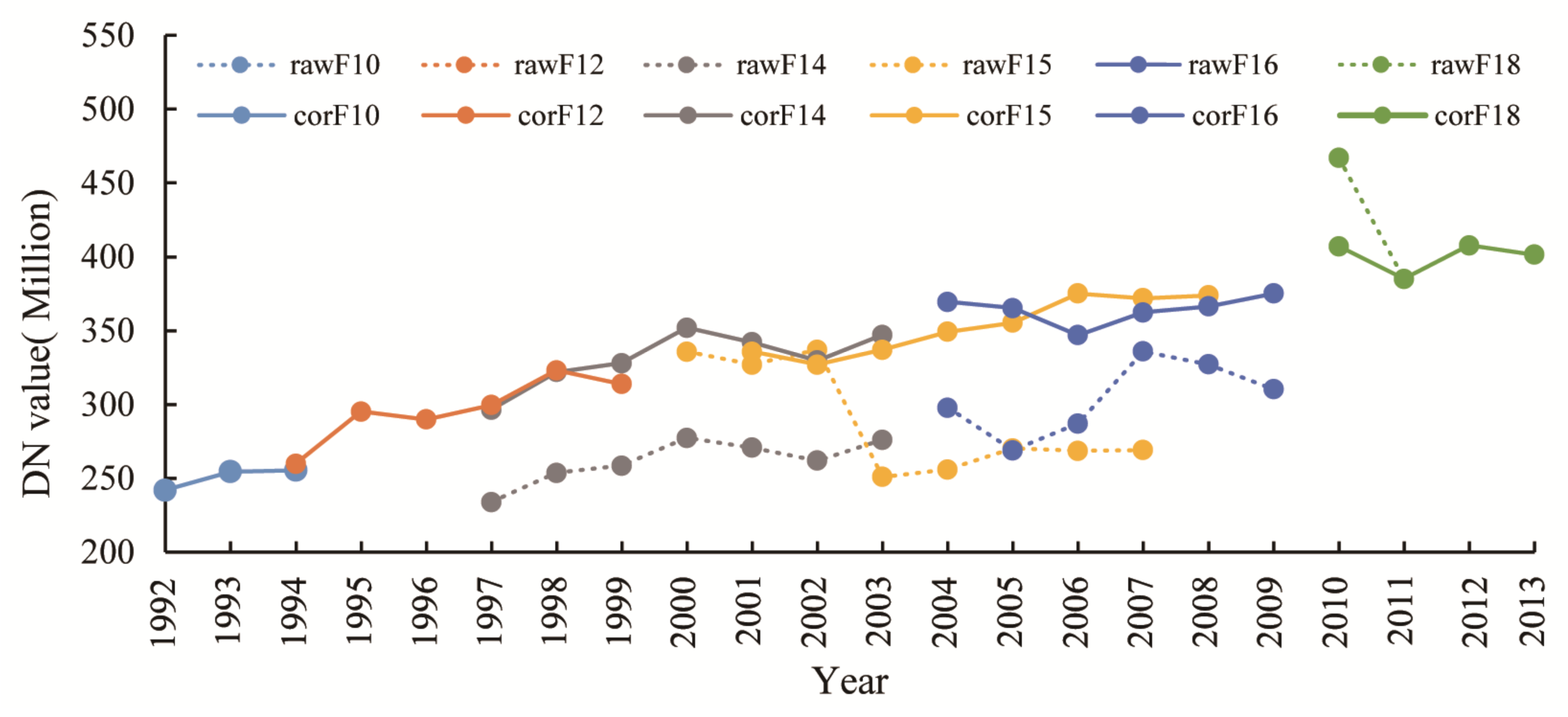
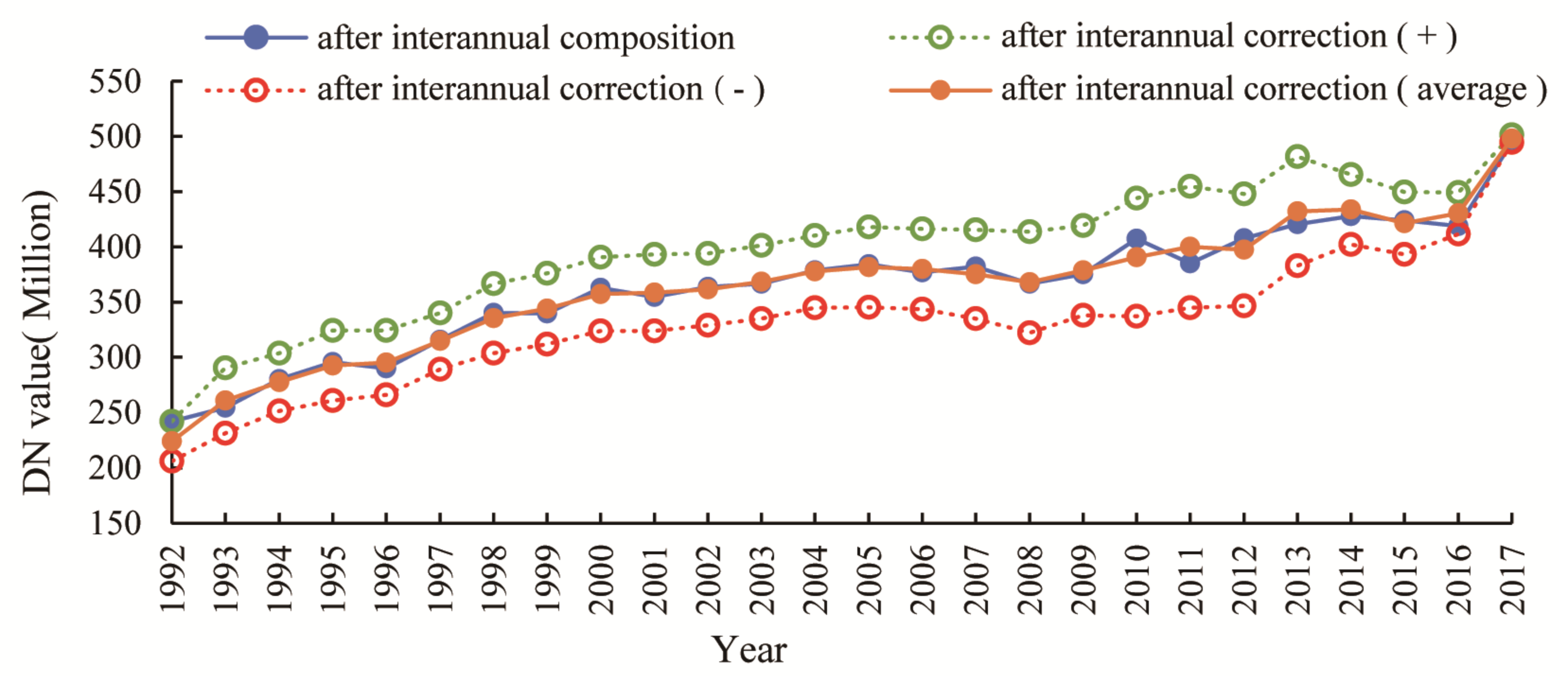
2.2. Preparation of the Long Time Series Nighttime Light Data

The DMSP-OLS sensors mounted on different satellites have different sensitivities to nighttime illumination and experience varying degrees of sensor degradation, and the DN values of nighttime light imagery obtained from different OLS sensors or from the same OLS sensor but in different years may vary in the same year [26] (raw dataset; the dashed line in Figure 1). In 2017, Li and Zhou et al. [19] proposed a stepwise gradient calibration method for nighttime light data. According to the aforementioned method, the authors obtained global corrected lighting data from 1992 to 2013 (corrected dataset; the solid line in Figure 1). Considering that there were multiple issues in the DMSP-OLS data in certain years from 1992 to 2013, we identified pixels in overlapping years through the method of Liu et al. [35] and formed annual DMSP-OLS datasets.

For the raw NPP-VIIRS data, the NPP-VIIRS monthly mosaic data were first synthesized into annual average nighttime light data. Then, based on the spatial distribution of stable light pixels and the principle of probability statistics, outliers were eliminated from the original datasets (such as fire points, volcanoes, and other background noise) [14,36]. During processing, considering the spatial matching with DMSP-OLS, the authors applied the nearest neighbor method to resample the original 500-m resolution images to a resolution of 1 km. Finally, the authors employed an exponential regression model to correct the annual NPP-VIIRS data to the DN range of the DMSP-OLS data.

Considering that the human economy and various energy consumption sources are generally increasing on a global scale, it is commonly believed that later DN values of nighttime light images should be at least larger than, or equal to, previous DN values in time series nighttime light datasets [35]. Based on this principle, Liu et al. [35] proposed a logical verification and correction method for time series data whereby, in time series nighttime light analysis, if a later DN value is smaller than an earlier DN value, the later DN value is then assigned the maximum value. However, in specific regions and periods, especially due to wars, abandonment of residential areas, economic downturns, factory closures, etc., the above assumptions are not applicable, and the nighttime lights corrected by this principle may exhibit notable deviations [37]. For this reason, Zhao et al. [12] proposed a method of simultaneously performing two logical tests and final averaging so that the positive (the green line in Figure 2) and negative (the red line in Figure 2) deviations cancel each other. The corrected time series data (the orange line in Figure 2) are more in line with reality.

For more details on the long-term nighttime light dataset preparation process, please refer to Supplementary material 1.

2.3. Analytical Method

This study first referred to the World Bank’s regionalization scheme and combined the lower-level administrative divisions (provinces and states) of relevant countries in key regions (see Supplementary material 2) to analyze the spatial characteristics of global nighttime lights.

This paper also analyzed the temporal and spatial evolution characteristics of the low-brightness zone (LBZ), medium-brightness zone (MBZ), and high-brightness zone (HBZ). Based on the distribution characteristics of the pixel brightness frequency in 1992 (excluding the 0-value zone), the nighttime light thresholds of the above three types of areas were determined as follows: LBZ: (0,6); MBZ: (6,10); and HBZ: (10~63) (see Supplementary material 3). When quantifying these three types of lighting areas, the world’s largest lighted area was first determined based on all the lighting data from 1992 to 2017. Thereafter, within the maximum lighted area, the specific spatial locations of the above three types of areas in the different years were determined.

The authors mainly analyzed indicators such as the total nighttime lights (TNL) and the nighttime lighting area (NLA). For the change in TNL, the temporal trend was further analyzed, and the Mann-Kendall significance test was conducted. In addition, significant differences in the nighttime light spatial distribution were also analyzed, and the adopted indicator was the coefficient of variation (CV).

The TNL is the cumulative sum of the DN values of all pixels in one nighttime light image of an area, defined as:

$$TN{L}_i={\displaystyle {\sum }_{j=1}^{N_i}D{N}_{ij}}$$

(1)

where DN_ij is the DN value of the j-th grid in the i-th country, and N_i is the total number of grids in the i-th country.

The NLA is the total area of all pixel grids with light pixel DN values larger than 0, defined as:

$$NL{A}_i={\displaystyle {\sum }_{j=1}^{N_i}N{L}_{Area}}$$

(2)

where NL_Area is the area of each pixel grid, and N_i is the total number of grids in the i-th country.

The CV is a normalized measure of the degree of data dispersion, defined as the ratio of the standard deviation to the mean:

$$CV=\frac{\sqrt{{\displaystyle {\sum }_{i=1}^N{\left(TN{L}_i-\overline{TNL}\right)}^2/N}}}{\overline{TNL}}\times 100\%$$

(3)

where CV is the dispersion degree of the regional nighttime lights, TNL_i is the sum of the DN values of the i-th area, $\overline{TNL}$ is the mean of the DN values of the overall area, and N is the total number of areas.

The CV reflects the relative difference between the data and the overall average value [38]. The larger the CV, the higher the degree of deviation and the larger the difference between regions; conversely, the data are more balanced and a small difference occurs among the different regions [39].

3. Results

3.1. The World Is Getting Brighter

The global TNL increased from 2.1 × 10⁸ in 1992 to 4.7 × 10⁸ in 2017. The global TNL in 2017 was 2.2 times that of 1992, with an annual growth rate of 3.2%. Compared to 1992, approximately 40.3% of the global lighting areas became brighter in 2017, but 8.1% of the lighting areas became darker. The total increase in global TNL is 2.5 × 10⁸, which is equivalent to approximately 3.05 times the United States TNL in 2017. The total area of the global brightening region is 1.7 × 10⁷ km², which is equivalent to approximately 1.1 times the area of the United States. At the global scale, a land area of 1.3 × 10⁷ km² transitioned from an unlighted area to a lighted area, which is equivalent to 0.8 times the area of the United States.

There are 5 areas where the nighttime lights had significantly brightened (Figure 3), namely, eastern and coastal China, Southeast Asia, South Asia (SAS), the Persian Gulf, and the Mediterranean (see Supplementary material 3 for the regional division and statistics of each region).

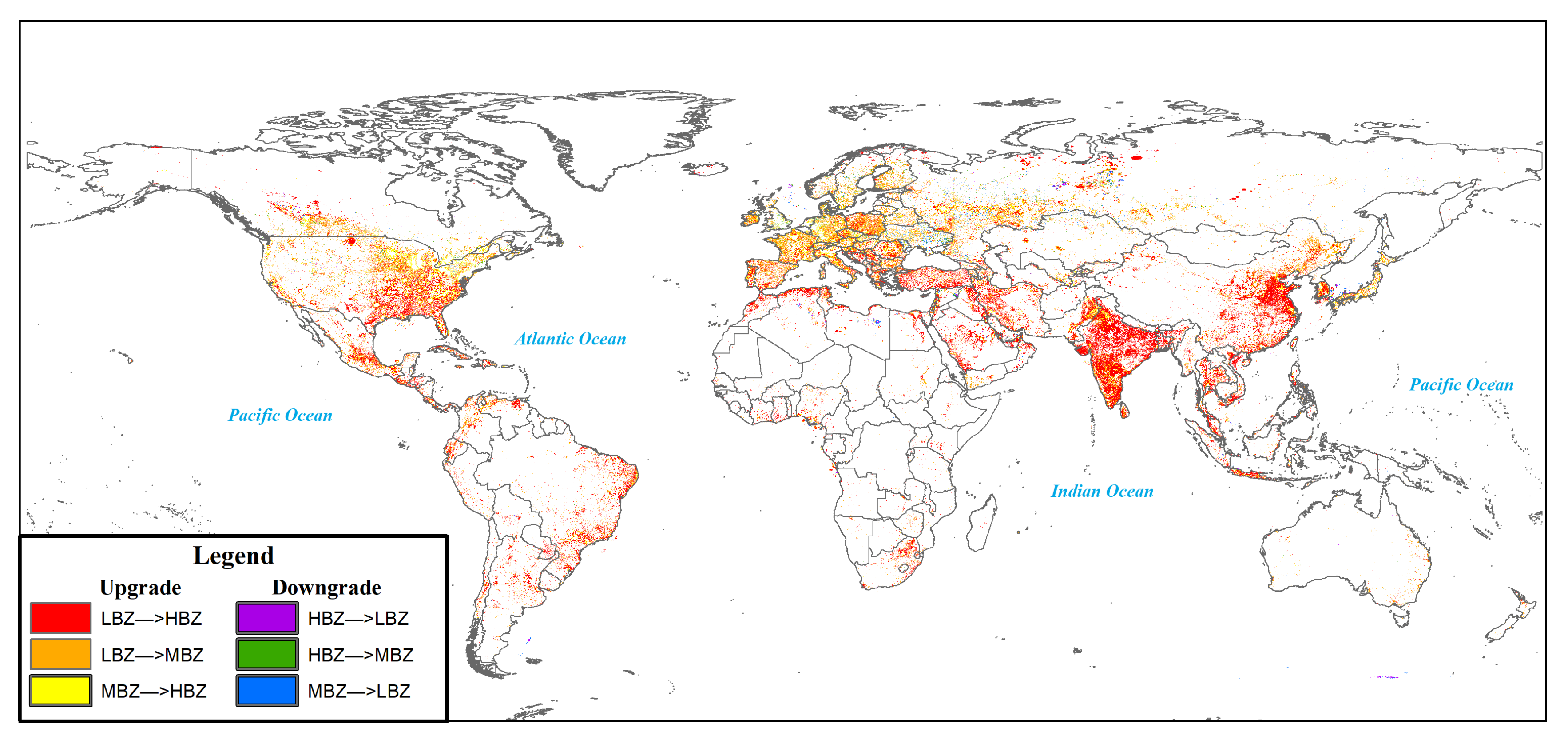
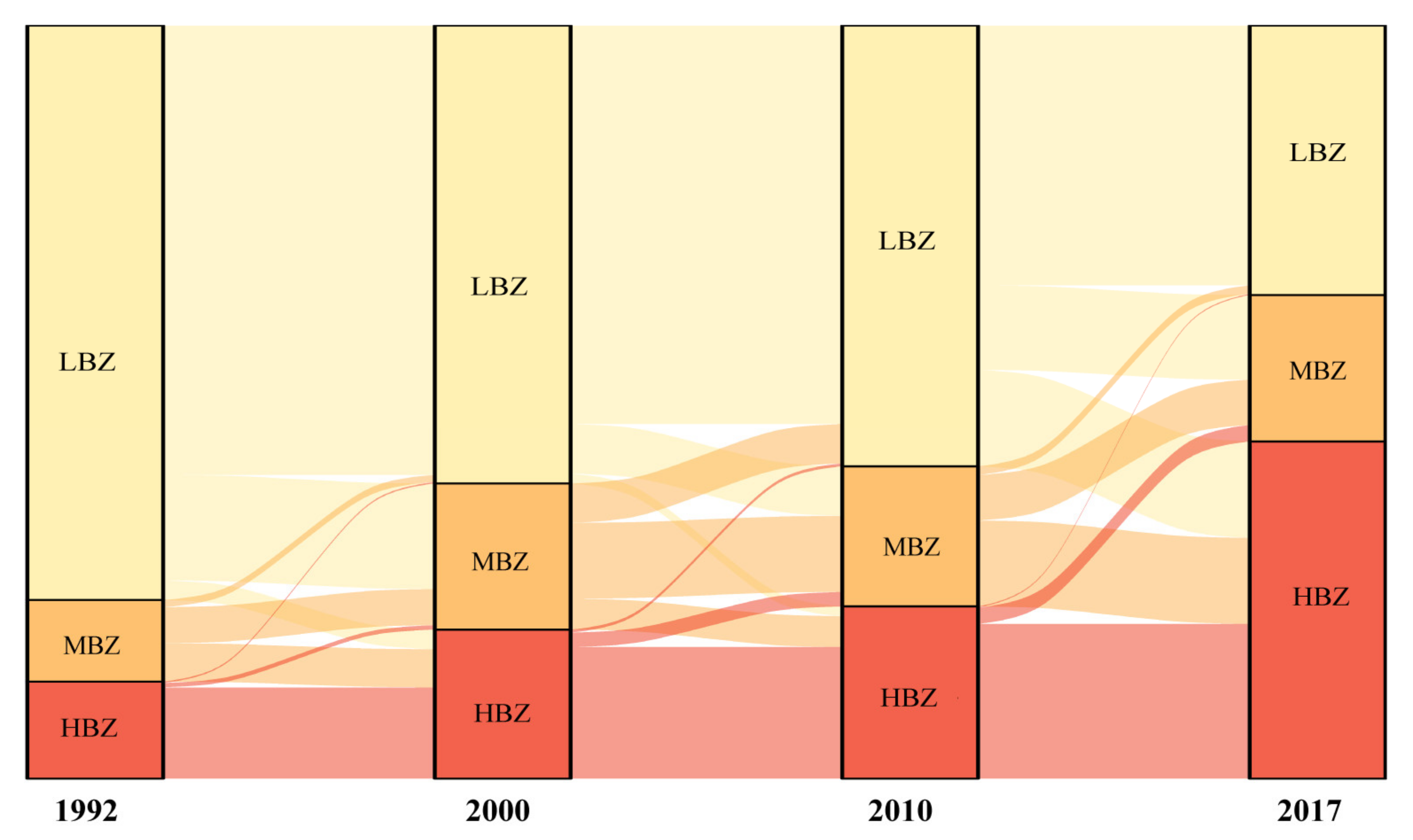
3.2. Low-Brightness Zones Quickly Brightened, and The Global Brightness Became More Uniform

Over the past 26 years, the global nighttime lights have transitioned from a low brightness to a high brightness (Figure 4 and Figure 5).

The TNL in the LBZ increased 2.2 × 10⁸, accounting for 85.7% of the global TNL increase, and 78.0% of the global brightened areas occurred in the LBZ. According to the long time series (26 years from 1992 to 2017), the area converted from an LBZ into an HBZ accounted for 50.9% of the LBZ change area, while the area converted from an LBZ into an MBZ accounted for 31.0% of the LBZ change area.

The TNL in the MBZ increased 3.2 × 10⁷, accounting for 12.4% of the global TNL increase, and 12.7% of the global brightened areas was located in the MBZ. The transition process from an LBZ to an HBZ generally involved conversion into an MBZ first, followed by the change to an HBZ (Figure 5).

As global nighttime lights have become brighter, they are more evenly distributed across space. The main reason is that the nighttime lights in the LBZ have significantly increased, and the CV value in the LBZ has significantly decreased. The CV of the nighttime lights in the global lighted areas decreased from 210% in 1992 to 117% in 2017. The CV of the nighttime lights in the LBZ decreased from 213% in 1992 to 115% in 2017. The CV of the nighttime lights did not change much in the MBZ and HBZ, and the CV of the nighttime lights in the MBZ was between 13% and 70%, while the CV in the HBZ varied between 60% and 65%.

3.3. China, India, and the United States Lead Global Brightening

According to the increase in TNL or bright areas, the world’s most powerful economy (the United States) and two prominent emerging economies (China and India) have led the global brightening trend (

Table 1. Statistics of the nighttime light stocks and variations in major countries from 1992 to 2017.

Rank	TNL in 2017 (Million)	Largest Lighting Area (Million km2)	TNL Increase (Million)	Ratio of the TNL Increase (%)	Ratio of the Bright Area (%)	Ratio of the Darkening Area (%)	Area from Unlighted to Lighted (million km2)
1	United States (83.8)	United States (6.6)	China (34.9)	China (13.7)	United States (13.3)	Russia (22.8)	China (1.48)
2	China (44.1)	Russia (5.6)	India (30.9)	India (12.1)	China (12.6)	United States (22.1)	United States (1.39)
3	Russia (40.0)	China (4.0)	United States (28.6)	United States (11.2)	India (10.8)	Canada (11.8)	Russia (1.38)
4	India (38.4)	India (2.9)	Russia (14.7)	Russia (5.8)	Russia (7.2)	Ukraine (7.1)	India (1.24)
5	Canada (17.03)	Canada (2.0)	Brazil (12.8)	Brazil (5.0)	Brazil (4.1)	United Kingdom (3.5)	Brazil (0.66)
6	Brazil (16.98)	Brazil (1.5)	Iran (8.6)	Iran (3.4)	Iran (3.1)	Sweden (3.2)	Canada (0.40)
7	Iran (12.0)	Iran (0.98)	Turkey (7.8)	Turkey (3.1)	Mexico (2.6)	Japan (2.7)	Turkey (0.38)
8	France (10.0)	Mexico (0.94)	Saudi Arabia (6.7)	Saudi Arabia (2.6)	France (2.5)	India (2.3)	Iran (0.33)
9	Mexico (9.6)	France (0.88)	Mexico (6.3)	Mexico (2.5)	Turkey (2.3)	China (1.8)	Mexico (0.30)
10	Saudi Arabia (9.2)	Ukraine (0.82)	Canada (4.3)	Canada (1.7)	Poland (2.2)	Finland (1.5)	Poland (0.25)

Notes: The ratio of the total nighttime lights (TNL) increase is the ratio of the TNL increase in each country to the global TNL increase. (1) The ratio of the bright area is the ratio of the bright area in each country to the global total bright area. (2) The ratio of the darkening area is the ratio of the darkening area in each country to the global total darkening area. (3) The area from unlighted to lighted is the area where the DN value has changed from zero to nonzero (>0).

).

In terms of the increase in TNL, from 1992 to 2017, China’s TNL increased 3.5 × 10⁷. Over the past 26 years, the Chinese TNL increased 4.8 times. The average annual growth rate of the TNL is as high as 6.48%, which is double the growth rate of the global TNL. The newly added TNL was equivalent to 41.7% of the United States’ TNL in 2017, accounting for 13.7% of the global TNL increase over the same period. The TNL of India increased 3.0 × 10⁷, second only to China, and the Indian TNL increased 5.1 times. The average annual growth rate of the TNL is slightly higher than that of China (6.73%), which is 2.1 times the global TNL growth rate. The increased TNL is equivalent to 36.9% of the United States’ TNL in 2017, accounting for 12.1% of the global TNL increase over the same period. The United States’ TNL increased 2.9 × 10⁷, an increase of 1.52 times. The average annual growth rate of the TNL is 1.69%, which is approximately half of the global TNL average annual growth rate. The increased TNL is equivalent to 34.2% of the United States’ TNL in 2017, accounting for 11.2% of the global TNL increase over the same period.

From the perspective of the bright area, from 1992 to 2017, the United States has the largest light-emitting area, which is approximately 0.23 × 10⁷ km², accounting for 13.3% of the global bright area over the same period, and the bright area is equivalent to 14.4% of the area of the United States. The Chinese bright area is 0.22 × 10⁷ km², which is smaller than that of the United States, accounting for 12.6% of the global bright area over the same period, and the bright area is equivalent to 13.6% of that of the United States. The bright area of India is 0.19 × 10⁷ km², which is second to that of China, accounting for 10.8% of the global bright area over the same period, and the Indian bright area is equivalent to 11.7% of that of the United States.

It should be pointed out that the United States, as the world’s most powerful economy, has the largest TNL value and lighting area. From 1992 to 2017, the United States brightened area was 0.23 × 10⁷ km², which is the largest in the world. However, the proportion of the brightened area to the largest lighting area of the United States has been lower than that of China and India for many years. In the United States, this proportion has been 34.9% for many years, while the proportion in China is 55.1%. In India, the above proportion is as high as 65.2%. In addition, significant darkening has occurred in the United States. Approximately 0.78 × 10⁶ km² of the United States’ lighting area exhibited a darkening trend, accounting for 11.7% of the country’s largest persistent lighting area and 22.1% of the total global darkening area. In contrast, China has experienced significant darkening in only 0.06 × 10⁶ km² (1.5% of the country’s largest persistent lighting area, accounting for 1.8% of the global darkening area), while India has experienced significant darkening in 0.08 × 10⁶ km² (2.7% of the country’s largest persistent lighting area, accounting for 2.3% of the global darkening area).

The TNL of the United States was 8.4 × 10⁷ in 2017, while the TNL of China was only 4.4 × 10⁷, and the TNL of India was 3.8 × 10⁷. Considering the average annual growth rate of the TNL over the past 26 years (1.69% in the United States, 6.48% in China, and 6.73% in India), it is expected that China and India will surpass the United States in approximately 13.9 and 16.1 years, respectively, or by approximately 2031 and 2033, respectively.

In addition, from 1992 to 2017, 0.15 × 10⁷ km² of Chinese land (accounting for 37.3% of the country’s largest persistent lighting area) was converted from a completely unlighted area into a lighted area, while in India, 0.12 × 10⁷ km² of land (accounting for 42.7% of the country’s largest persistent lighting area) was converted from a completely unlighted area into a lighted area. In the United States, a land area of 0.14 × 10⁷ km² (accounting for 20.9% of the country’s largest persistent lighting area) was converted from a completely unlighted area into a lighted area. Therefore, compared to the rapid urbanization process in China and India, the urbanization process in the United States has basically ended, and it can be inferred that in the future, more unlighted areas in China and India will be converted into lighted areas. Furthermore, in India, 72.1% of the land area has already been converted into a lighted area, while this value is only 29.0% in China. Therefore, we believe that the Chinese TNL has more room for growth than that of India and the United States.

4. Discussion

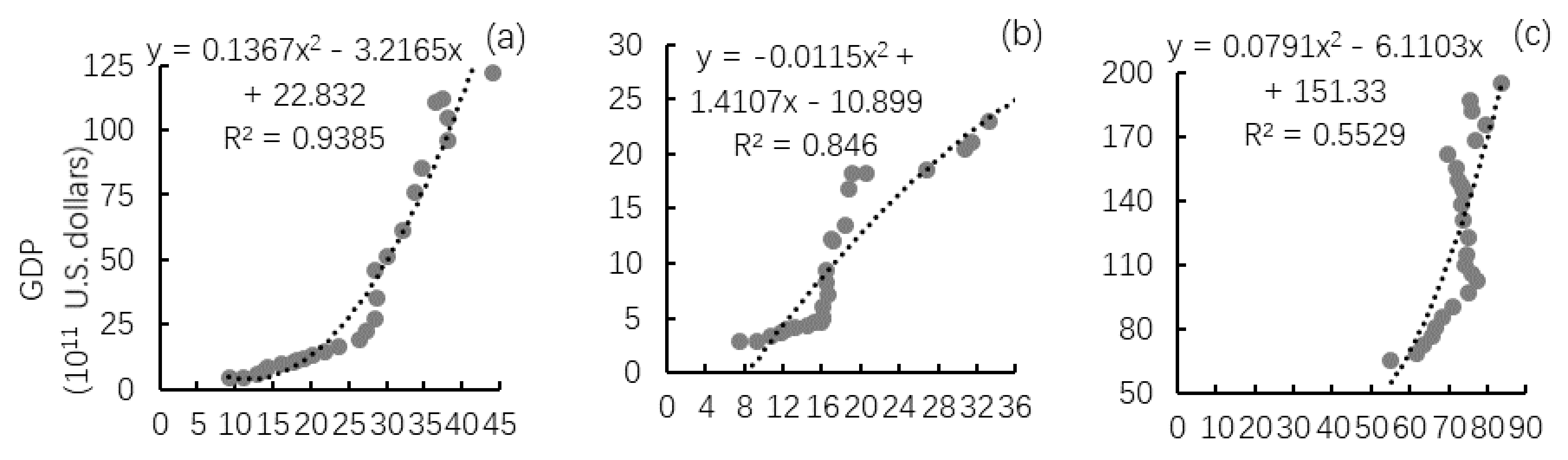
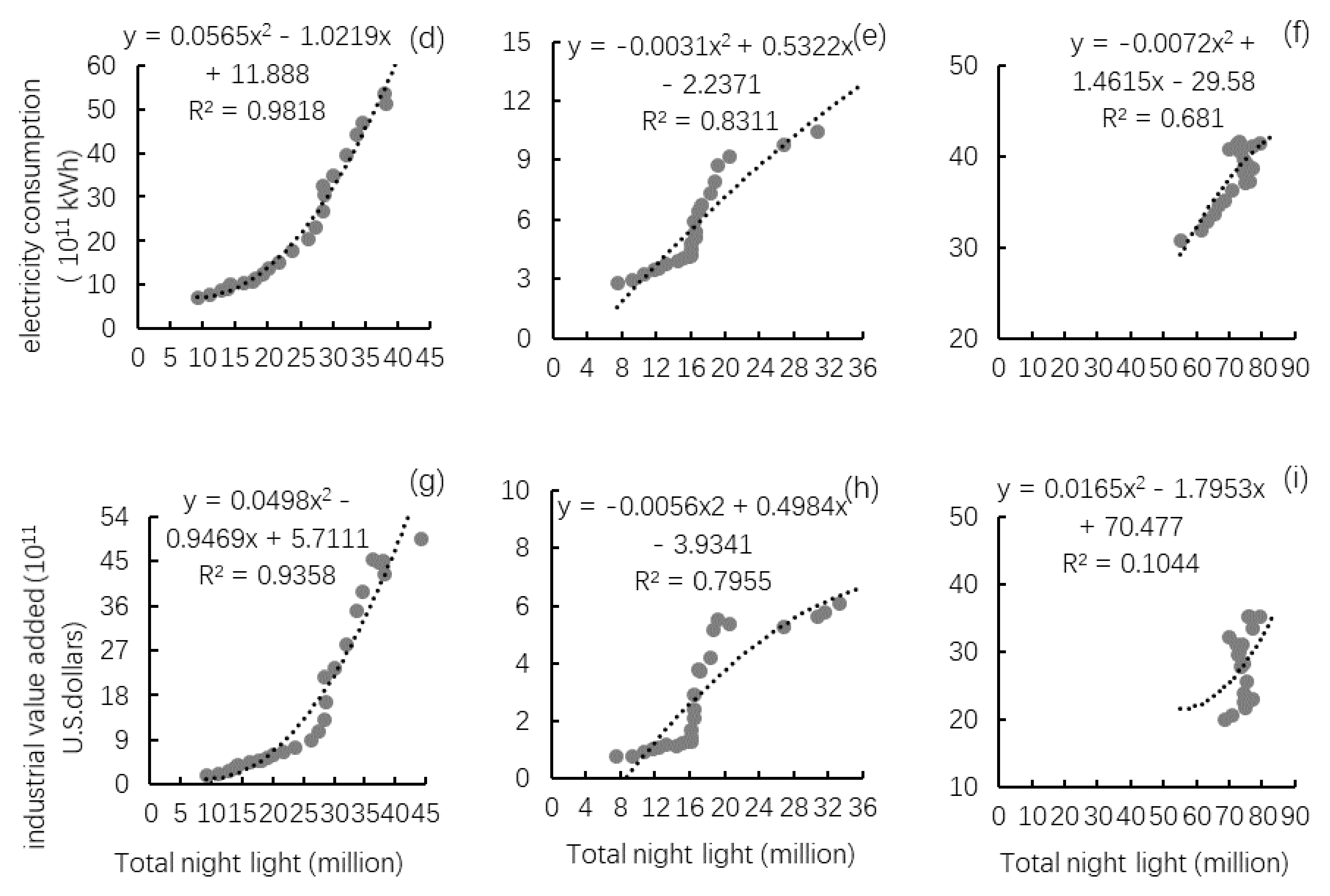
4.1. Relationship between Nighttime Lights and Economic Development

In the two emerging economies (China and India), the regional TNL values are closely related to the GDP, industrial added value, and electricity consumption (Figure 6). The coefficient of determination obtained by regression analysis is very high (that of China is above 0.93, while that of India is above 0.79). In China, according to the regression analysis between the TNL and the GDP, industrial added value, and electricity consumption, the determination coefficients are 0.939, 0.982 and 0.936, respectively. In India, the above three coefficients are 0.846, 0.831, and 0.796, respectively. However, in mature, developed economies (i.e., the United States), the correlation between the TNL and the above indicators has rapidly declined. The correlation between the electricity consumption and TNL is the highest, with a determination coefficient of 0.681. The correlation between the GDP and nighttime lights has rapidly decreased, and the correlation between the industrial added value and TNL is the lowest (the determination coefficient of the former is 0.553, while that of the latter is only approximately 0.1).

From the perspective of national industrial development, the United States economy has long left the industrialization stage and entered the stage of industrial informatization and services in approximately 2000 [40,41]. Because the U.S. economy relies mainly on high-end service industries and high-tech information industries, which do not require large-scale and intense illumination (electricity is still required but not necessarily for lighting purposes), the correlation between the TNL and the GDP and industrial added value is not high. Correspondingly, in China and India, as two emerging economies, the development stage is still in the industrialization stage. Their national economic development relies heavily on traditional industrial industries with a high energy consumption, high heat generation, and high illumination requirements [42].

Related studies have shown that the use of nighttime lights can overcome the fluctuations in price and currency exchange rate, and that they are suitable for the observation and comparison of economic activities in different regions over long periods [43]. Nighttime lights also record the informal or underground economy, reflecting the economic activity more fully [44]. The studies by Dai et al. [3] show that nighttime lights are related to the economic index at the regional scale. Our research results further reveal that when conducting nighttime light simulation to analyze national economic-related indicators, it is necessary to consider factors such as the industrial development stage and the industrial development structure of the target country.

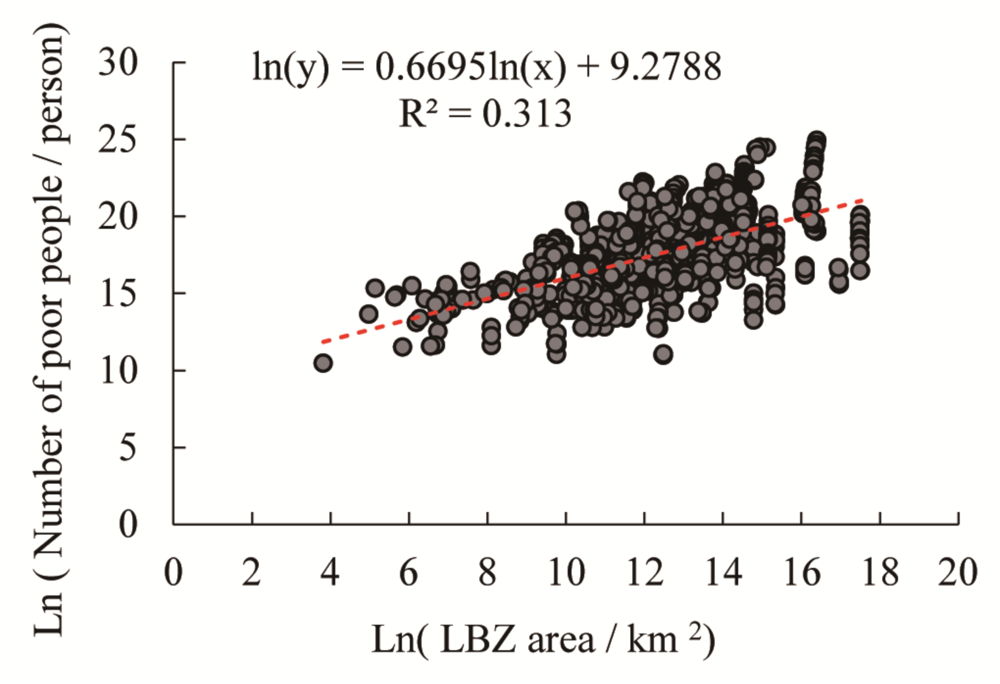
4.2. Relationship between the LBZ Area and Global Poverty Reduction

According to statistics of the World Bank [45], from 1993 to 2015, the absolute number of people living in extreme poverty worldwide dropped from 1.89 × 10⁹ to 0.73 × 10⁹, and the global poverty rate declined from 34% to 9.9%, a decrease of 24.1%. Over the same period, the proportion of the global LBZ area in the global lighting area decreased from 73.3% (3.2 × 10⁷ km²) to 44.5% (1.9 × 10⁷ km²), a decrease of 28.8%. Clearly, at the global scale, the area ratio of the LBZ has declined synchronously with the global poverty rate. At the national and regional scales, there also exists a close relationship between the LBZ area and the population living in extreme poverty in each country (Figure 7).

In terms of the spatial distribution pattern, in 1993, SAS had the highest proportion of the LBZ area to the largest lighting area (87.3%), followed by sub-Saharan Africa (SSF) (86.2%) and East Asia and the Pacific (EAS) (84.6%). In 2015, the LBZ areas in SAS and EAS significantly decreased, and the proportions of the LBZ area to the regional largest lighting area decreased to 28.6% and 49.2%, respectively. While the proportion of the LBZ in SSF has also decreased, it still remains the highest in the world at 59.3% (

Table 2. Statistics of the LBZ area changes and poverty population in major global regions from 1993 to 2015.

Rank	1993				2015
	LBZ Area (Million km2)	Proportion of the LBZ (%)	Poverty Rate (%)	People Living in Extreme Poverty (Billion)	LBZ Area (Million km2)	Proportion of the LBZ (%)	Poverty Rate (%)	LBZ Area (Million km2)
1	ECS 10.5	SAS 87.3	SSF 59.6	EAS 10.2	ECS 7.5	SSF 59.3	SSF 41	SSF 4.1
2	EAS 5.6	SSF 86.2	EAS 53.7	SAS 5.4	EAS 3.3	LCN 50.0	SAS 12.4	SAS 2.2
3	NAC 5.2	EAS 84.6	SAS 44.9	SSF 3.3	NAC 3.1	EAS 49.2	MEA 4.2	EAS 0.53
4	LCN 3.6	LCN 83.7	LCN 14	LCN 0.66	LCN 2.1	ECS 48.5	LCN 3.9	LCN 0.25
5	SAS 3.1	MEA 80.6	MEA 7	ECS 0.44	MEA 1.4	MEA 42.4	EAS 2.3	MEA 0.18
6	MRA 2.7	ECS 67.2	ECS 5.2	MEA 0.19	SAS 1.0	NAC 36.4	ECS 1.5	ECS 0.14
7	SSF 1.1	NAC 60.0	NAC 0	NAC 0	SSF 0.7	SAS 28.6	NAC 0	NAC 0

Notes: (1) SSF is sub-Saharan Africa, MEA is Middle East and North Africa, SAS is South Asia, LCN is Latin America and the Caribbean, NAC is North America, EAS is East Asia and the Pacific, ECS is Europe and Central Asia. (2) The proportion of LBZ is the proportion of the LBZ area to the largest lighting area in this area for many years.

). The changes in the absolute LBZ proportion and their ranking are consistent with relevant conclusions in the World Bank report. In particular, the global poverty center has shifted from Asia to the African continent, and Africa, especially SSF, has become the main global battlefield for poverty reduction [45].

In particular, in EAS, the proportion of the Chinese LBZ area in its largest lighting area decreased from 89.1% to 48.5%, a decrease of 40.6%. Considering that the Chinese lighting area is only 9.2% of the global lighting area, China’s LBZ reduction accounts for 13.0% of the global LBZ reduction. This indicates that the Chinese LBZ area has been substantially reduced, which has greatly shifted the center of gravity in EAS and the global LBZ spatial distribution. China has made important contributions to the realization of global antipoverty goals.

4.3. Uncertainty

With the use of the overlaying characteristics of the various DMSP/OLS satellites in the time series, the authors realized nighttime light dataset correction at the global scale based on time continuity. In contrast to the general calibration method based on reference images [28], the method applied in this paper modifies the original DN value less, and the corrected and original data have a similar brightness, which eventually ensures that the data of the same year, from different satellites, or the same satellite, in various years, are more comparable [19].

With the application of the exponential regression model and the nearest neighbor sampling method, the authors corrected the NPP-VIIRS dataset with high spatial and radiation resolutions to the DMSP-OLS dataset with relatively low spatial and radiation resolutions. This occurred because the DMSP-OLS dataset is a longer time series, and the upscaling conversion method is relatively easy to implement [46]. In the future, it is important to perform timing matching and superresolution fusion analysis of the DMSP-OLS and NPP-VIIRS data, which will greatly expand the application scope and capability of the DMSP-OLS data [18].

In the real world, with economic activities shifting from rural to urban areas, scattered rural lights will gradually weaken and shift to the surrounding cities, while the wars in certain areas will lead to a sharp reduction or even complete disappearance of nighttime lights. Although it is reasonable to assume that the global TNL will increase monotonically, this assumption is not valid at the pixel or small-region scale. In this study, a two-way correction and averaging method was adopted. Although this route can avoid sudden changes in the nighttime light distribution, it may also cause unnecessary changes in the true DN value of pixels.

The national- and regional-scale models built between the nighttime light data and the GDP and other economic indicators perform well, but these models are usually unable to depict rural and urban areas or estimate small-scale areas properly. This is mainly due to the low spatial and radiation resolutions of DMSP-OLS sensors. In poor areas, vast rural areas, and small-scale areas, the number of effective pixels is very small [47], while in prosperous urban areas, the low radiation and spatial resolutions of the DMSP-OLS sensors lead to light saturation or lighting spillover effects [48]. Different stages of economic development and industry composition will affect the correlation between the economic indicators and nighttime lights [49].

Antipoverty is a large and complex system involving many aspects [50]. Although this study has confirmed a close relationship between the LBZ and poor populations, other studies have also demonstrated that light data can be coupled with other geographic background data to evaluate the spatial location and poverty levels in poor areas [51,52]. However, in general, the relationship between nighttime lights and poverty is solely an empirical relationship, and the TNL indicator may be a weak agent of poverty at the cluster level [53,54]. However, the advantages of nighttime light data, due to their easy access, spatial comparability, repeated measurements, and high spatial resolution, still make them a great resource for poverty assessment [55].

5. Conclusions

From 1992 to 2017, the global nighttime lights have gradually increased. This increase is mainly concentrated in five areas, including the eastern and coastal China, the Southeast Asia, the South Asia, the Persian Gulf, the Mediterranean. The brightness of the LBZ has significantly increased, with more than half of the global nighttime light growth occurring in past LBZ regions. The significant increase in brightness in the LBZ is also the reason for the more uniform brightness of the global nighttime lights. The world’s most powerful economies (United States) and emerging economies (China and India) have led the global brightening trend, and over the next 20-30 years, the total number of nighttime lights in China and India is expected to exceed that of the United States. Our study has also found that brightness changes are closely related to economic indicators such as GDP growth, industrial development, and electricity consumption increase, and this relationship is more notable in countries at the industrialization stage. In addition, the LBZ maintains the same trend as that of the poverty rate at the global and national scales, and the change in the global LBZ center indicates the spatial shift of global key high-poverty regions.

References

1. Hu, K.; Qi, K.; Guan, Q.; Wu, C.; Yu, J.; Qing, Y.; Zheng, J.; Wu, H.; Li, X. A Scientometric Visualization Analysis for Night-Time Light Remote Sensing Research from 1991 to 2016. Remote Sens. 2017, 9, 802. [Google Scholar] [CrossRef] [Green Version]
2. Doll, C.N.; Muller, J.P.; Morley, J.G. Mapping regional economic activity from night-time light satellite imagery. Ecol. Econ. 2006, 57, 75–92. [Google Scholar] [CrossRef]
3. Dai, Z.; Hu, Y.; Zhao, G. The Suitability of Different Nighttime Light Data for GDP Estimation at Different Spatial Scales and Regional Levels. Sustainability 2017, 9, 305. [Google Scholar] [CrossRef] [Green Version]
4. Witmer, F.D.W.; O’Loughlin, J. Detecting the Effects of Wars in the Caucasus Regions of Russia and Georgia Using Radiometrically Normalized DMSP-OLS Nighttime Lights Imagery. GIScience Remote Sens. 2011, 48, 478–500. [Google Scholar] [CrossRef]
5. Small, C.; Pozzi, F.; Elvidge, C. Spatial analysis of global urban extent from DMSP-OLS night lights. Remote Sens. Environ. 2005, 96, 277–291. [Google Scholar] [CrossRef]
6. Xie, Y.; Weng, Q. Spatiotemporally enhancing time-series DMSP/OLS nighttime light imagery for assessing large-scale urban dynamics. ISPRS J. Photogramm. Remote Sens. 2017, 128, 1–15. [Google Scholar] [CrossRef]
7. Bennie, J.; Davies, T.; Duffy, J.; Inger, R.; Gaston, K.J. Contrasting trends in light pollution across Europe based on satellite observed nighttime lights. Sci. Rep. 2014, 4, 3789. [Google Scholar] [CrossRef] [Green Version]
8. Letu, H.; Nakajima, T.; Nishio, F. Regional-Scale Estimation of Electric Power and Power Plant CO2 Emissions Using Defense Meteorological Satellite Program Operational Linescan System Nighttime Satellite Data. Environ. Sci. Technol. Lett. 2014, 1, 259–265. [Google Scholar] [CrossRef]
9. Li, X.; Zhan, C.; Tao, J.; Li, L. Long-Term Monitoring of the Impacts of Disaster on Human Activity Using DMSP/OLS Nighttime Light Data: A Case Study of the 2008 Wenchuan, China Earthquake. Remote Sens. 2018, 10, 588. [Google Scholar] [CrossRef] [Green Version]
10. Coscieme, L.; Sutton, P.; Anderson, S.; Liu, Q.; Elvidge, C.D. Dark Times: Nighttime satellite imagery as a detector of regional disparity and the geography of conflict. GIScience Remote Sens. 2016, 54, 118–139. [Google Scholar] [CrossRef]
11. Shi, K.; Yu, B.; Huang, Y.; Hu, Y.; Yin, B.; Chen, Z.; Chen, L.; Wu, J. Evaluating the Ability of NPP-VIIRS Nighttime Light Data to Estimate the Gross Domestic Product and the Electric Power Consumption of China at Multiple Scales: A Comparison with DMSP-OLS Data. Remote Sens. 2014, 6, 1705–1724. [Google Scholar] [CrossRef] [Green Version]
12. Zhao, N.; Zhou, Y.; Samson, E.L. Correcting Incompatible DN Values and Geometric Errors in Nighttime Lights Time-Series Images. IEEE Trans. Geosci. Remote Sens. 2014, 53, 2039–2049. [Google Scholar] [CrossRef]
13. Baugh, K.; Hsu, F.-C.; Elvidge, C.D.; Zhizhin, M. Nighttime Lights Compositing Using the VIIRS Day-Night Band: Preliminary Results. In Proceedings of the 35th Asia-Pacific Advanced Network, Manoa, HI, USA, 13–18 January 2013; Asia-Pacific Advanced Network: Manoa, HI, USA, 2013; Volume 35, pp. 70–86. [Google Scholar] [CrossRef] [Green Version]
14. Elvidge, C.D.; Baugh, K.; Zhizhin, M.; Hsu, F.C.; Ghosh, T. VIIRS night-time lights. Int. J. Remote Sens. 2017, 38, 5860–5879. [Google Scholar] [CrossRef]
15. Li, X.; Xu, H.; Chen, X.; Li, C. Potential of NPP-VIIRS Nighttime Light Imagery for Modeling the Regional Economy of China. Remote Sens. 2013, 5, 3057–3081. [Google Scholar] [CrossRef] [Green Version]
16. Elvidge, C.; Hsu, F.-C.; Baugh, K.; Ghosh, T. National Trends in Satellite-Observed Lighting: 1992–2012. Remote Sens. Nat. Res. 2014, 20144266, 97–120. [Google Scholar] [CrossRef]
17. Wu, J.; He, S.; Peng, J.; Li, W.; Zhong, X. Intercalibration of DMSP-OLS night-time light data by the invariant region method. Int. J. Remote Sens. 2013, 34, 7356–7368. [Google Scholar] [CrossRef]
18. Pandey, B.; Zhang, Q.; Seto, K.C. Comparative evaluation of relative calibration methods for DMSP/OLS nighttime lights. Remote Sens. Environ. 2017, 195, 67–78. [Google Scholar] [CrossRef]
19. Li, X.; Zhou, Y. A stepwise calibration of global DMSP/OLS stable nighttime light data (1992–2013). Remote Sens. 2017, 9, 637. [Google Scholar]
20. Zhang, X.; Wu, J.; Peng, J.; Cao, Q. The Uncertainty of Nighttime Light Data in Estimating Carbon Dioxide Emissions in China: A Comparison between DMSP-OLS and NPP-VIIRS. Remote Sens. 2017, 9, 797. [Google Scholar] [CrossRef] [Green Version]
21. Shao, X.; Cao, C.; Zhang, B.; Qiu, S.; Elvidge, C.; von Hendy, M. Radiometric calibration of DMSP-OLS sensor using VIIRS day/night band. In Earth Observing Missions and Sensors: Development, Implementation, and Characterization III; SPIE: Beijing, China, 2014; Volume 92640A. [Google Scholar] [CrossRef]
22. Zhu, X.; Ma, M.-G.; Yang, H.; Ge, W. Modeling the Spatiotemporal Dynamics of Gross Domestic Product in China Using Extended Temporal Coverage Nighttime Light Data. Remote Sens. 2017, 9, 626. [Google Scholar] [CrossRef] [Green Version]
23. Li, X.; Li, D.; Xu, H.; Wu, C. Intercalibration between DMSP/OLS and VIIRS night-time light images to evaluate city light dynamics of Syria’s major human settlement during Syrian Civil War. Int. J. Remote Sens. 2017, 38, 5934–5951. [Google Scholar] [CrossRef]
24. Pok, S.; Matsushita, B.; Fukushima, T. An easily implemented method to estimate impervious surface area on a large scale from MODIS time-series and improved DMSP-OLS nighttime light data. ISPRS J. Photogramm. Remote Sens. 2017, 133, 104–115. [Google Scholar] [CrossRef] [Green Version]
25. Li, C.; Li, G.; Zhu, Y.; Ge, Y.; Kung, H.-T.; Wu, Y. A likelihood-based spatial statistical transformation model (LBSSTM) of regional economic development using DMSP/OLS time-series nighttime light imagery. Spat. Stat. 2017, 21, 421–439. [Google Scholar] [CrossRef]
26. Ji, G.; Zhao, J.; Yang, X.; Yue, Y.; Wang, Z. Exploring China’s 21-year PM10 emissions spatiotemporal variations by DMSP-OLS nighttime stable light data. Atmos. Environ. 2018, 191, 132–141. [Google Scholar] [CrossRef]
27. Shi, K.; Yu, B.; Huang, C.; Wu, J.; Sun, X. Exploring spatiotemporal patterns of electric power consumption in countries along the Belt and Road. Energy 2018, 150, 847–859. [Google Scholar] [CrossRef]
28. Elvidge, C.D.; Ziskin, D.; Baugh, K.E.; Tuttle, B.T.; Ghosh, T.; Pack, D.W.; Erwin, E.H.; Zhizhin, M. A Fifteen Year Record of Global Natural Gas Flaring Derived from Satellite Data. Energies 2009, 2, 595–622. [Google Scholar] [CrossRef]
29. Zhou, N.; Hubacek, K.; Roberts, M. Analysis of spatial patterns of urban growth across South Asia using DMSP-OLS nighttime lights data. Appl. Geogr. 2015, 63, 292–303. [Google Scholar] [CrossRef]
30. Yang, W.; Luan, Y.; Liu, X.; Yu, X.; Miao, L.; Cui, X. A new global anthropogenic heat estimation based on high-resolution nighttime light data. Sci. Data 2017, 4, 170116. [Google Scholar] [CrossRef]
31. Tripathy, B.R.; Tiwari, V.; Pandey, V.; Elvidge, C.D.; Rawat, J.S.; Sharma, M.P.; Prawasi, R.; Kumar, P. Estimation of Urban Population Dynamics Using DMSP-OLS Night-Time Lights Time Series Sensors Data. IEEE Sensors J. 2017, 17, 1013–1020. [Google Scholar] [CrossRef]
32. Zhang, Q.; Seto, K.C. Mapping urbanization dynamics at regional and global scales using multi-temporal DMSP/OLS nighttime light data. Remote Sens. Environ. 2011, 115, 2320–2329. [Google Scholar] [CrossRef]
33. Mills, S.; Weiss, S.; Liang, C. VIIRS day/night band (DNB) stray light characterization and correction. In Earth Observing Systems XVIII; SPIE: San Diego, CA, USA, 2013; Volume 88661P. [Google Scholar] [CrossRef]
34. Wu, R.; Yang, D.; Dong, J.; Zhang, L.; Xia, F. Regional Inequality in China Based on NPP-VIIRS Night-Time Light Imagery. Remote Sens. 2018, 10, 240. [Google Scholar] [CrossRef] [Green Version]
35. Liu, Z.; He, C.; Zhang, Q.; Huang, Q.; Yang, Y. Extracting the dynamics of urban expansion in China using DMSP-OLS nighttime light data from 1992 to 2008. Landsc. Urban Plan. 2012, 106, 62–72. [Google Scholar] [CrossRef]
36. Chen, Z.; Yu, B.; Hu, Y.; Huang, C.; Shi, K.; Wu, J. Estimating House Vacancy Rate in Metropolitan Areas Using NPP-VIIRS Nighttime Light Composite Data. IEEE J. Sel. Top. Appl. Earth Obs. Remote Sens. 2015, 8, 2188–2197. [Google Scholar] [CrossRef]
37. Liu, L.; Leung, Y. A study of urban expansion of prefectural-level cities in South China using night-time light images. Int. J. Remote Sens. 2015, 36, 5557–5575. [Google Scholar] [CrossRef]
38. Eldridge, S.; Ashby, D.; Kerry, S. Sample size for cluster randomized trials: Effect of coefficient of variation of cluster size and analysis method. Int. J. Epidemiol. 2006, 35, 1292–1300. [Google Scholar] [CrossRef] [Green Version]
39. Houser, K.W.; Wei, M.; Royer, M. Illuminance Uniformity of Outdoor Sports Lighting. Leukos 2011, 7, 221–235. [Google Scholar] [CrossRef]
40. Stiroh, K.J. Information Technology and the U.S. Productivity Revival: What Do the Industry Data Say? Am. Econ. Rev. 2002, 92, 1559–1576. [Google Scholar] [CrossRef] [Green Version]
41. Neely, A.; Neely, A.D. Exploring the financial consequences of the servitization of manufacturing. Oper. Manag. Res. 2008, 1, 103–118. [Google Scholar] [CrossRef] [Green Version]
42. Wang, Q.; Li, R. Drivers for energy consumption: A comparative analysis of China and India. Renew. Sustain. Energy Rev. 2016, 62, 954–962. [Google Scholar] [CrossRef]
43. Chen, X.; Nordhaus, W. Using luminosity data as a proxy for economic statistics. In Proceedings of the National Academy of Sciences; National Academy of Sciences: Washington, DC, USA, 2011; pp. 8589–8594. [Google Scholar]
44. Sutton, P.; Costanza, R. Global estimates of market and non-market values derived from nighttime satellite imagery, land cover, and ecosystem service valuation. Ecol. Econ. 2002, 41, 509–527. [Google Scholar] [CrossRef]
45. Group, W.B. Poverty and Shared Prosperity 2018: Piecing Together the Poverty Puzzle; World Bank Publications: Washington, DC, USA, 2018. [Google Scholar]
46. Wu, H.; Li, Z.-L. Scale Issues in Remote Sensing: A Review on Analysis, Processing and Modeling. Sensors 2009, 9, 1768–1793. [Google Scholar] [CrossRef] [PubMed]
47. Yu, B.; Shi, K.; Hu, Y.; Huang, C.; Chen, Z.; Wu, J. Poverty Evaluation Using NPP-VIIRS Nighttime Light Composite Data at the County Level in China. IEEE J. Sel. Top. Appl. Earth Obs. Remote Sens. 2015, 8, 1–13. [Google Scholar] [CrossRef]
48. Li, X.; Zhou, Y. Urban mapping using DMSP/OLS stable night-time light: A review. Int. J. Remote Sens. 2017, 38, 6030–6046. [Google Scholar] [CrossRef]
49. Bennett, M.; Smith, L.C. Advances in using multitemporal night-time lights satellite imagery to detect, estimate, and monitor socioeconomic dynamics. Remote Sens. Environ. 2017, 192, 176–197. [Google Scholar] [CrossRef]
50. Pan, J.; Hu, Y. Spatial Identification of Multi-dimensional Poverty in Rural China: A Perspective of Nighttime-Light Remote Sensing Data. J. Indian Soc. Remote Sens. 2018, 46, 1093–1111. [Google Scholar] [CrossRef]
51. Chen, X. Explaining Subnational Infant Mortality and Poverty Rates: What Can We Learn from Night-Time Lights? Spat. Demogr. 2015, 3, 27–53. [Google Scholar] [CrossRef]
52. Elvidge, C.D.; Sutton, P.; Ghosh, T.; Tuttle, B.T.; Baugh, K.; Bhaduri, B.; Bright, E. A global poverty map derived from satellite data. Comput. Geosci. 2009, 35, 1652–1660. [Google Scholar] [CrossRef]
53. Wang, W.; Cheng, H.; Zhang, L. Poverty assessment using DMSP/OLS night-time light satellite imagery at a provincial scale in China. Adv. Space Res. 2012, 49, 1253–1264. [Google Scholar] [CrossRef]
54. Proville, J.; Zavala-Araiza, D.; Wagner, G. Night-time lights: A global, long term look at links to socio-economic trends. PLoS ONE 2017, 12, e0174610. [Google Scholar] [CrossRef] [Green Version]
55. Noor, A.; Alegana, V.A.; Gething, P.W.; Tatem, A.J.; Snow, R.W. Using remotely sensed night-time light as a proxy for poverty in Africa. Popul. Health Metrics 2008, 6, 5. [Google Scholar] [CrossRef] [Green Version]
Figure 1. The annual sums of the digital number (DN) values of the Defense Meteorological Satellites Program/Operational Linescan System (DMSLP/OLS) dataset before and after correction. The correction method proposed by Li and Zhou et al. [19] was applied to correct the DN values of the nighttime light data from the 6 different sensors (F10, F12, F14, F15, F16, and F18) in various years. After correction, the annual sum of the DN values exhibits reduced fluctuations between years and a higher consistency.
Sustainability 12 04905 g001
Figure 2. The annual sums of the DN values of the DMSP-OLS and the Suomi National Polar-Orbiting Partnership Visible Infrared Imaging Radiometer Suite (NPP-VIIRS) datasets before and after interannual correction. The positive and negative deviations cancel each other based on the correction method proposed by Zhao et al. [12]. The corrected and input annual data deviate very little and essentially show a steady increase.
Sustainability 12 04905 g002
Figure 3. Change tendency of the global nighttime lights from 1992 to 2017. The legend shows the slope of the interannual change in nighttime lights (DN/year). The blank area indicates no light or significance test failure (Mann-Kendall test, at P ≤ 0.05). The black ellipses highlight 5 areas where the nighttime lights have significantly brightened, namely, eastern and coastal China, Southeast Asia, South Asia, the Persian Gulf, and the Mediterranean. From 1992 to 2017, a global area of 1.3 × 10⁷ km2 changed from an unlighted area to a lighted area, equivalent to 0.8 times the area of the United States.
Sustainability 12 04905 g003
Figure 4. Changes in the global nighttime light zones from 1992 to 2017. LBZ—>MBZ indicates the transition from the low-brightness zone to the medium-brightness zone; LBZ—>HBZ indicates the transition from the low-brightness zone to the high-brightness zone; MBZ—>LBZ indicates the transition from the medium-brightness zone to the low-brightness zone; MBZ—>HBZ indicates the transition from the medium-brightness zone to the high-brightness zone; HBZ—>LBZ indicates the transition from the high-brightness zone to the low-brightness zone; and HBZ—>MBZ indicates the transition from the high-brightness zone to the medium-brightness zone.
Sustainability 12 04905 g004
Figure 5. Changes in the global nighttime light level from 1992 to 2017. LBZ, MBZ, and HBZ are the low-, medium- and high-brightness zones, respectively. The height of the column and the line width of the node indicate the area and conversion size, respectively, between the LBZ, MLZ and HBZ in 1992, 2000, 2010 and 2017.
Sustainability 12 04905 g005
Figure 6. Correlation between the TNL and economic indicators. (a) the TNL and GDP of China; (b) the TNL and GDP of India; (c) the TNL and GDP of United States; (d) the TNL and electricity consumption of China; (e) the TNL and electricity consumption of India; (f) the TNL and electricity consumption of United States; (g) the TNL and industrial added value of China; (h) the TNL and industrial added value of India; (i) the TNL and industrial added value of United States. The TNL values in the two emerging economies (China and India) exhibit a close relationship with the economic indicators, while the TNL in mature, developed economies (United States) has a poor relationship with the economic indicators.
Sustainability 12 04905 g006aSustainability 12 04905 g006b
Figure 7. Scatterplot of the LBZ area and the population living in extreme poverty. From 1993 to 2015, there exists a close relationship between the LBZ area and the number of people living in extreme poverty in each country, namely, a logarithmic linear relationship.
Sustainability 12 04905 g007