mD-Resilience: A Multi-Dimensional Approach for Resilience-Based Performance Assessment in Urban Transportation

Abstract

As demonstrated for extreme events, the resilience concept is used to evaluate the ability of a transportation system to resist and recover from disturbances. Motivated by the high cumulative impact of recurrent perturbations on transportation systems, we have investigated resilience quantification as a performance assessment method for high-probability low-impact (HPLI) disturbances such as traffic congestions. Resilience-based metrics are supplementary to conventional travel-time-based indices in literature. However, resilience is commonly quantified as a scalar variable despite its multi-dimensional nature. Accordingly, by hypothesizing increased information gain in performance assessment, we have investigated a multi-dimensional approach (mD-Resilience) for resilience quantification. Examining roadways’ resilience to recurrent congestions as a contributor to sustainable mobility, we proposed to measure resilience with several attributes that characterize the degradation stage, the recovery stage, and possible recovery paths. These attributes were integrated into a performance index by using Data Envelopment Analysis (DEA) as a non-parametric method. We demonstrated the increased information gain by quantifying the performance of major freeways in Los Angeles, California using Performance Measurement System (PeMS) data. The comparison of mD-Resilience approach with the method based on area under resilience curves showed its potential in distinguishing the severity of congestions. Furthermore, we showed that mD-Resilience also characterizes performance from the lens of delay and bottleneck severities.

1. Introduction

Resilience concept has been traditionally used in the context of extreme events to evaluate the operation of transportation systems. It is clear that extreme disastrous events can dramatically impact the mobility and the performance of transportation systems; however, high-probability low-impact (HPLI) disturbances can also play an important role in reducing the efficiency of such systems, mainly in the form of congestions, which in turn have a significant impact on sustainable mobility. HPLI disturbances not only cause delays and inconvenience, but also result in negative consequences such as air and noise pollution, high energy consumption, lower safety levels, and significant economic loss. These disturbances can happen due to numerous reasons such as bad weather [1], poor condition of local infrastructure [2], different speed regimes, the high volume of traffic [3], or infrastructure design and operational configurations. Conventional methods of performance assessment in transportation systems account for mobility and reliability by leveraging quantification methods that center around travel time as an important factor for travel efficiency. Mobility-based indices quantify how mobility is affected compared to normal operational conditions, and reliability measures help plan according to affected travels. Several indices are used for the purpose of quantification including Travel Time Index (TTI), Travel Delay, Level of Service (LOS), and Buffer Index, among others. These metrics provide information on the severity of potential problems at different spatiotemporal scales. However, from an operational standpoint, it is important to understand how roadways withstand disturbances followed by congestions, and how they recover from such disturbances to the normal performance level. This could be viewed from the lens of resilience.

In the transportation domain, the resilience of a system reflects on attributes such as redundancy (multiple components with similar functionality), diversity (components with diverse functionalities), robustness, rapidity, or safety [4,5,6]. The existing resilience studies in the transportation domain are primarily focused on supply-chain management and logistical operations aspects [7] for major disturbances. On the other hand, recurrent HPLI disrupting events, such as traffic jams, have been less explored from the resilience perspective despite their considerable cumulative impact. Evaluating transportation system performance based on their resilience provides information on the behavior of roadways in coping with the imbalance considering the above attributes. This fact highlights the importance of studying the resilience of roadways to HPLI events in addition to using conventional metrics for performance assessments. In other words, the resilience concept could be utilized to provide supplementary information on how a system degrades and recovers, and potentially uncover the causes of system performance variations during congestions.

A common approach to characterize and quantify the resilience of a system is based on the resilience curve [8], which is typically presented as a system performance indication curve plotted against time. Research studies mainly use the area under the resilience curve (from the time the disturbance occurs until the system is recovered) as an indicator of resilience; the area above the curve is called performance or resilience loss. However, this approach only considers the total loss of the system performance—also referred to as the “impact of disruption”—while resilience has multiple dimensions that could show the behavior of a system from different perspectives. Accordingly, we hypothesized that a multi-dimensional approach for quantifying complex resilience behavior of roadways across multiple stages of a resilience curve (i.e., degradation, absorption, and recovery) could result in higher information gain in performance assessment compared to solely relying on measuring the impact of disruption. Therefore, we proposed a process of multi-dimensional resilience (mD-Resilience) assessment for quantification of relative resilience across different roadway sections to assess their vulnerability to disturbances. This approach accounts for several attributes from the performance curve, as well as their aggregation (through Data Envelopment Analysis) as a scalar performance index. In this way, individual features and the aggregate score could be leveraged in assessing the performance.

Through a case study on three regions in major freeways of the Los Angeles metropolitan area and by leveraging the data from Performance Measurement System (PeMS), we have investigated how accounting for a multi-dimensional resilience-based scoring approach (mD-Resilience) could add value to the process of performance assessment for roadways and the associated decision-making. Through this case study, we have shown how the proposed resilience quantification technique could be also used to characterize the severity of conventional performance assessment techniques, such as delays and bottlenecks while providing a supplementary metric for assessment. In doing so, the remainder of this study is organized as follows. Section 2 reviews the background pertinent to this research. We present the details of the proposed methodology in Section 3. To illustrate the application of the proposed approach and answer the research questions, the case study on the Los Angeles area freeways is presented in Section 4. Finally, the discussion of results and the conclusion are presented in Section 5 and Section 6, respectively.

2. Research Background

In the transportation domain, several performance metrics are used to measure the likelihood, the time, and the severity of roadways’ congestions. In general, measures aimed at investigating and reducing congestion should account for statistical techniques, replicability of the results, and the ability to describe the existing traffic [9,10]. Conventional methods of congestion assessment could be divided into two categories of mobility-based and reliability-based. The former refers to the metrics that are used to quantify and characterize the severity of reduction in mobility, and the latter focuses on probabilistic planning to mitigate the impact of congestion. In both cases, quantification metrics center around measuring the impact on travel time. Speed-based metrics (besides average travel speed) have been widely suggested in the literature. For instance, speed reduction index as the ratio of the decline in the speed from the free flow condition [11] and Corridor Mobility Index (CMI) [12] as the product of travel speed and peak-hour person volume per lane have been suggested as measures of congestion. Travel Time Index (TTI), as the most applied time-based congestion measure, compares peak period travel and free flow travel [13] and provides guidance on identifying major issues. Travel Rate Index (TRI) computes the ratio of additional time needed for a trip due to congestion [14]. There is also another set of measures based on the demand and capacity relation, such as Level of Service (LOS), which are more interpretable by the public audience. The LOS metric represents location-specific congestion, not the overall or regional congestion condition.

In addition to evaluating the performance, these metrics have been leveraged for investigating the mitigation strategies. For example, Gong and Fan [15] proposed an approach for identification and ranking of recurrent bottlenecks in freeways using the reliability of travel time. Roshan and Mitra [16] leveraged the commercial GPS fleet management devices in trucks to identify and classify bottleneck locations at highways based on the variation of speed. Moreover, Mishra et al. [17] used empirical travel time data from INRIX [18] to estimate travel time reliability. As these studies demonstrate, the conventional and long-established descriptors provide valuable information for characterizing the severity of congestion problems in roadways. However, they do not provide sufficient information on how the performance degrades (characterizing resistance to loss) and recovers (characterizing the ability to return to normal operations). These characteristics could be represented in the context of resilience.

As noted, in the transportation domain, resilience has been studied for the transport-related areas of logistics and supply chain management [19], as well as organizational and economic perspectives [20], and socioeconomic impacts [21], specifically in case of extreme events and disasters [22,23]. While resilience analysis concerning roadways and networks has been the subject of several studies (e.g., [24,25,26,27]), the study of traffic flow and recurrent congestions have been briefly addressed in the literature [7]. The existing research almost exclusively focused on the resilience of networks in the case of disasters [28,29,30,31]. Nevertheless, some authors have recognized the importance and leveraged the concept of resilience to characterize the performance of roadways for HPLI events. Tang et al. [25] constructed a congestion metric based on the resilience engineering concept and transport science to quantify recurrent congestions’ severity based on spatiotemporal traffic patterns. They demonstrated that their proposed metric is comparable to conventional congestion quantification metrics, such as Level of Service and Relative Congestion Index, while providing some additional information. In another study, Calvert and Snelder [7] presented the Link Performance Index for Resilience (LPIR), as an analytically developed scalar performance index, to evaluate the resilience level of individual road sections relative to a road network by accounting for resistance and recovery characteristics for minor disturbances like daily-based congestions. They visually compared the LPIR values with recovery time and the total delay of the roadways and specified that this metric provides additional information compared to the delay. Compared to the existing literature, our proposed contribution is a data-driven method that accounts for various features from the performance curve to characterize different stages of resilience. This method provides supplementary information in comparison to the conventional metrics of performance measurement, while it could be used to infer the severity of delay and bottlenecks.

Multi-dimensionality of resilience in the transportation domain has been emphasized and discussed from different perspectives. Murray-Tuite [4] identified ten dimensions to characterize resilience including redundancy, diversity, efficiency, autonomous components, strength, collaboration, adaptability, mobility, safety, and ability to recover quickly. The study highlights the importance of resilience for daily events, as well as extreme events, and defines a resilient transportation system as the one with the ten mentioned characteristics. Nevertheless, general approaches to study the resilience of transportation systems and roadways evaluate resilience based on one or both of the following perspectives [32]: (1) Resistance and ability to maintain functionality, and (2) rapidity and how fast the system recovers. Drawing on these perspectives, various metrics represented by recovery characteristics [7,24], the maximum deviation from the normal state [33,34], or network efficiency [35] have been suggested for resilience quantification. For instance, Twumasi-Boakye and Sobanjo [36] stated that resilience is measured by the entire performance loss from the occurrence of disaster to the full recovery of performance in a system. Liao et al. [37] proposed a time-dependent resilience metric, defined as the ratio of recovery at a given time to the function loss at a previous point in time. While such single dimensions simplify the analysis, they may not capture different aspects of a system’s response, as they often focus on one stage of disturbance (loss in performance or recovery) [38]. Hence, it is important to consider multiple dimensions simultaneously to better quantify a system’s overall ability to resist and recover from a disturbance [39].

Although not explicitly addressed in the transportation domain, the multi-dimensional resilience quantification has been previously addressed to a limited extent in urban area resilience to disasters by Zobel and Baghersad [38]. The authors characterized multiple dimensions of urban disaster resilience by leveraging the number of service calls. Their results showed the importance of considering multiple aspects of resilience (i.e., robustness and recovery time) in understanding the communities’ response to disasters. Nonetheless, other engineering and science disciplines have highlighted the importance of multi-dimensional resilience quantification. Therefore, we have proposed mD-Resilience to quantify the contribution of different resilience features, both individually and collectively, in evaluating the overall system resilience. The use of multiple aspects of performance when a disruption occurs will help gain a broader view of resilient behavior and provide a comprehensive method for added value in performance assessment and causation analysis as a supplementary source of information. To demonstrate these added values, we have utilized statistical measures of information gain and feature importance.

3. Materials and Methods

To address the research objectives, in developing the methodology, we have discussed the characteristics of the conventional resilience quantification methods to accentuate the need and importance of a multi-dimensional perspective in characterizing resilience. By leveraging the characteristics of a schematic performance curve of a system, we then proposed an approach for quantifying the resilience of roadway traffic from a multi-dimensional perspective. In doing so, and given the specific conditions of traffic flows on the roadways, we have accounted for two scenarios of (1) resilience to a single disturbance, and (2) resilience to a series of consecutive disturbances with temporal overlap.

3.1. Resilience Quantification

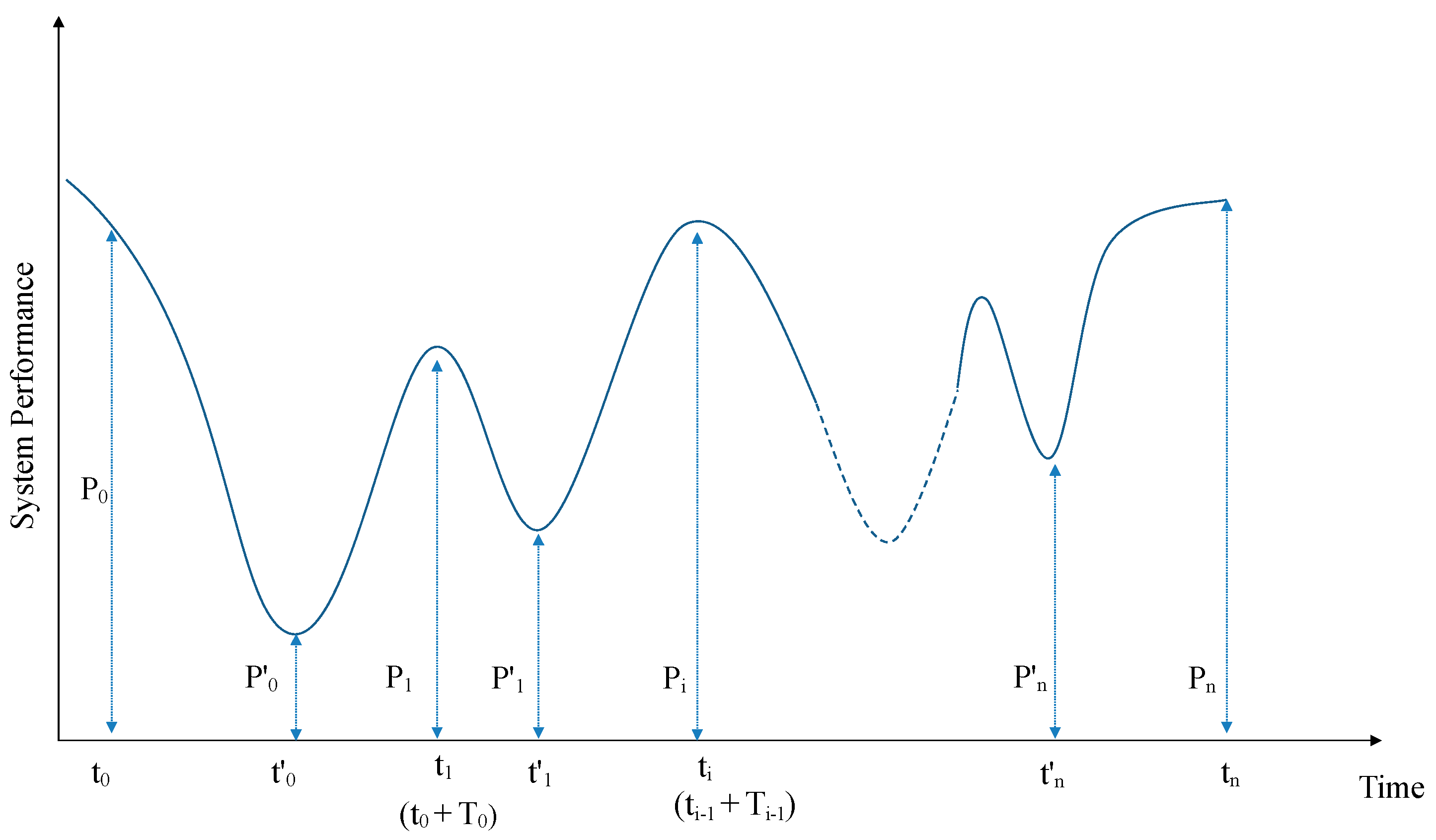
Like most engineered and infrastructure systems, roadways are exposed to minor and major disturbances and shocks. The disturbances result in the alteration of the system performance level over time. Facing a disturbance, the performance of the system first decreases (in a smooth or sudden path) and if resilient enough, it can recover from its disruptive state back to its operating state. There are four general stages that the resilience of a system is characterized with. The first stage is the normal state of operation with a performance of $P_0$ before a disturbance. The second stage, the degradation, is when the system performance degrades and starts to deteriorate down to the minimum level of ${P^{\prime }}_0$ following a disturbance at the time ($t_0$). Next, if not collapsed, the system starts to improve its performance in the recovery state, and the performance will get to the normal state (full recovery) or close to the normal state (partial recovery). Finally, the system performance reaches the newly recovered state and becomes stable. The characteristics of these four stages are what we have leveraged to propose the mD-Resilience metric.

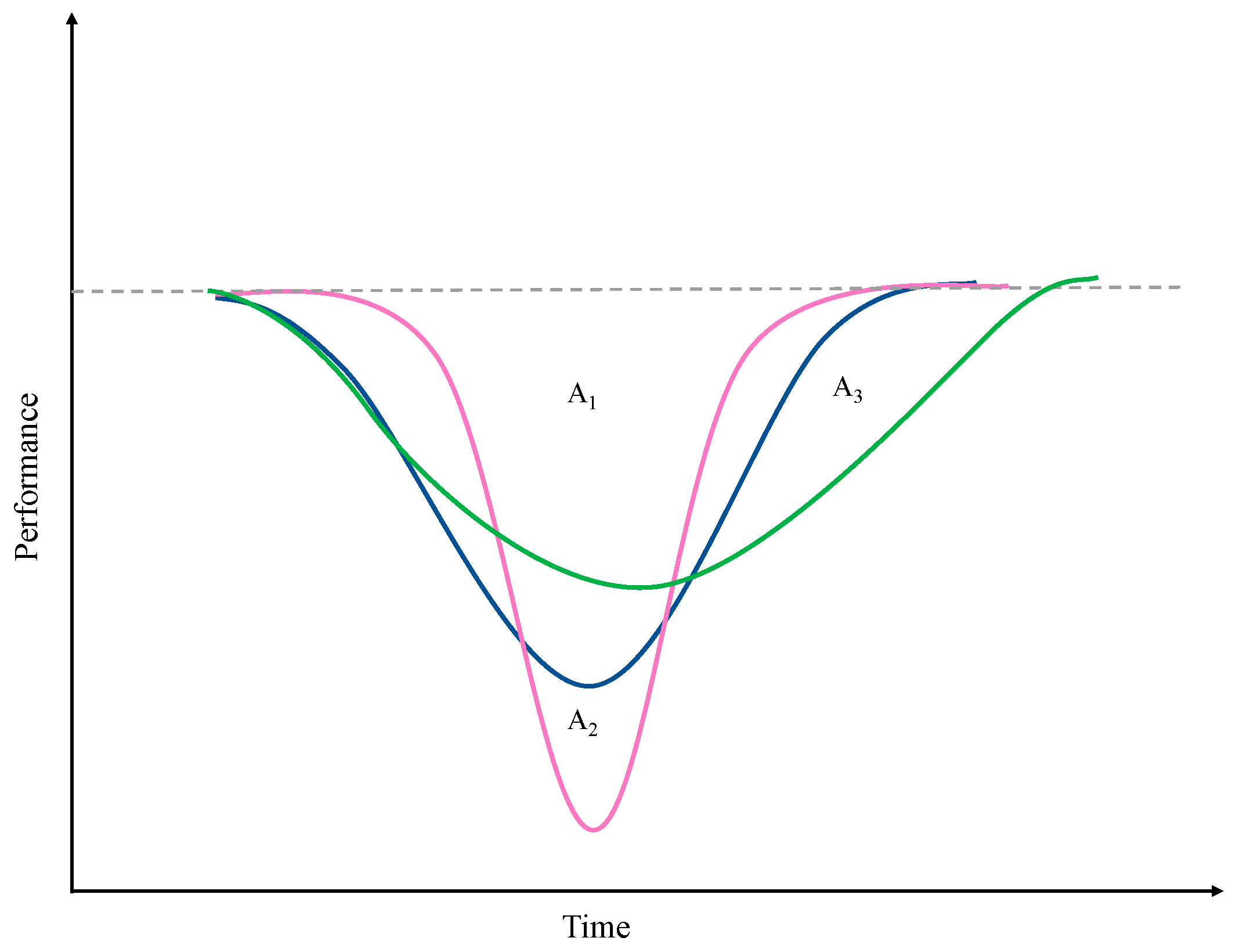
Multi-dimensional resilience quantification: Resilience has often been characterized using the area under the response curve (i.e., resilience triangle) [8]; a smaller area corresponds to a less resilient system. The area-based approach for quantification of performance loss provides insight into the general performance of the system. However, it could not provide enough information on characterizing the differences between two events—i.e., whether the loss is due to a long recovery (gain) time or it is due to an intense loss in performance. For example, the area of the resilience triangles is almost equal in Figure 1 ($A_1\approx A_2\approx A_3$). However, the rate of loss in performance and gain in performance (rate of recovery) are different, a reflection of different behavior of the system performance. In other words, there may be many different combinations of performance curve that results in the same total area under performance curves (quantified resilience). This is the foundation for our proposed investigation into the added value of the multi-dimensional resilience characterization approach. That is, the rate and intensity of the variations along the performance curve could be used to characterize the difference in resilience as a performance indicator. In addition to the area of the resilience triangle, other characteristics of the triangle (associated with different stages of loss and recovery) have been individually studied in different engineering disciplines [40,41]. However, in most complex systems, such as transportation systems, a single dimension might not be effective in characterizing the resilience and differentiating the relative performance of different components in a system.

Multi-event resilience quantification: Another important phenomenon of significant practical value in the context of this study is resilience characterization for consecutive events. Infrastructure systems, including transportation systems, may be prone to a sudden onset of a disturbance, followed by multiple sub-disturbances. Accordingly, a resilience quantification approach should also account for consecutive events and how they contribute to the overall resilience as individual single events.

3.2. Multi-Dimensional Resilience Indexing

Considering the above-mentioned factors, we have identified and defined a set of attributes that could better represent the functionality of a system when it comes to relative comparison of performance—specifically different sections in a roadway network in this study. These attributes include the attributes from existing literature across different engineering disciplines, as well as our defined attributes, including a modified characterization of resilience for multi-event circumstances. In what follows, we have presented the definitions, attributes, and the approach for combining these attributes as a single resilience score. Figure 2 illustrates a schematic performance curve and its evolution during a disruption event to show the variables used in the following definitions.

Definition 1—Robustness Range: System performance normally varies over time within a tolerable range, which is referred to as Robustness Range ($RR$) [42]. In other words, robustness refers to the stability of a system state within a range of performance. This range could be used in characterizing the range in which a decrement in performance is an actual congestion event rather than a random fluctuation of the traffic. In this study, we have adopted the definition of a congestion event from Tang et al. [25], which defined an event when the performance deteriorated out of the Robustness Range ($RR$). Likewise, a system is recovered when the performance returns to the robustness range. The RR is quantified as a percentage of performance at the normal stage ($P_0$).

Definition 2—Event: An event is characterized based on the temporal performance curve of a system (i.e., roadways in our study). Having $t_0$ as the start time of an event,$t_1$ is the time the performance is recovered to a new state of equilibrium, and ${t^{\prime }}_0$ (a time between $t_0$ and $t_1$) when the system starts to recover for which:

$$P\left({t^{\prime }}_0\right)\le P\left(t_i\right)\hspace{1em}\hspace{1em}\hspace{1em}\hspace{1em}\forall t_i\in \left(t_0,t_1\right)$$

(1)

then an event is characterized as [39]:

$$\forall t_i\in \left(t_0,t_1\right):\exists t_1:P\left(t_1\right)\ge P\left(t_i>{t^{\prime }}_0\right)ANDP\left(t_1\right)\ge \left(1-RR\right)\ast P_0$$

(2)

where $P$ is the performance of the system as a function of time.

3.2.1. Single Event Resilience Attributes

As noted, we have adopted and defined a number of attributes that could collectively characterize the effect of a disturbance and the response from a given system. These attributes are as follows:

Resistance (Re) indicates the impact of disturbance on the level of performance after degradation. Resistance gives a general insight into the non-operability of a system under disruptions. However, it does not convey information about how the system degrades following a disruptive event or how the recovery happens:

$$\mathrm{Re}=\frac{ {P^{\prime }}_0}{P_0}$$

(3)

Loss rate (L_R) is defined as the rate of drop in the performance during the degradation stage. L_R could provide information on the ability of a system to maintain its intended function. A smaller value of L_R means that the system shows more resistance to serviceability reduction, which is a desirable attribute:

$${\mathrm{L}}_{\mathrm{R}}=\frac{\left|{P^{\prime }}_0-P_0\right|}{{t^{\prime }}_0-t_0}$$

(4)

Recovery rate (R_R) is defined as the rate of gaining back the performance after reaching the minimum performance. The recovery rate can be derived from the performance curve from the time minimum performance happens until the time the system performance reaches its predefined normal level. Opposite to L_R, R_R could provide information on the ability of a system to get back to its intended function. The faster the system gets back to the intended operation level, the higher the R_R is:

$${\mathrm{R}}_{\mathrm{R}}=\frac{P_1-{P^{\prime }}_0}{t_1-{t^{\prime }}_0}$$

(5)

Event Duration (D) defines the time that takes for a draw-down and draw-up cycle to take place. It mainly indicates the time the system performance is not at the level it was intended and designed for:

$$\mathrm{D}=t_1-t_0$$

(6)

Recovery Percentage (R%) is an attribute that is used as a recovery path indicator. The recovery of a system after a disturbance could take different patterns and paths, leading to different recovery profiles. These differences in recovery are mostly due to the characteristics of a system (i.e., roadways in the context of this study). This concept has been depicted in Figure 2. Moving toward recovery to a stable state, three main scenarios could happen: Improved recovery, stable recovery, or deteriorated recovery. These potential recovery scenarios are quantified by Recovery Percentage, which is defined as the percentage of improvement in performance after the recovery, compared to the initial normal stage. Recovery percentage could provide information on the overall impact of the event on the system performance. Moreover, the recovery percentage indicates the recovery mode—i.e., full-recovery, partial recovery, or performance improvement:

$$\mathrm{R}\%=\frac{P_{1 }-P_0}{P_{0 }}\ast 100\%$$

(7)

3.2.2. Multi-Event Resilience Attributes

A multi-event disturbance refers to a condition in which a disturbance or shock to a system is followed by multiple related sub-disturbances. Such circumstances are complex, and they typically involve partial recoveries, and they need to balance multiple criteria for effective actions [43]. Figure 3 shows the schematic illustration of a multi-event disturbance.

Given a compound multi-event disturbance with n overlapping sub-disturbances, ${P^{\prime }}_i$ is the level of performance of the system after disturbance i occurs. Furthermore, $P_i$ is the performance level of the system before disturbance $\left(i+1\right)$ occurs, and $T_i$ is the duration from the state represented by $P_i$ to $P_{i+1}$ (i.e., duration for each partial recovery). Expanding on the single-event resilience attributes, in the generalized form, the multi-dimensional resilience attributes could be represented as follows:

Resistance (Re):

$$\mathrm{Re}=\frac{{\sum }_{i=0}^n\frac{P_i}{{P^{\prime }}_i}}{n}$$

(8)

Loss Rate (L_R):

$${\mathrm{L}}_{\mathrm{R}}=\frac{{\sum }_{i=0}^n\frac{|{P^{\prime }}_i-P_i|}{{t^{\prime }}_i-t_i}}{n}$$

(9)

Recovery Rate (R_R):

$${\mathrm{R}}_{\mathrm{R}}=\frac{{\sum }_{i=0}^n\frac{P_{i+1}-{P^{\prime }}_i}{t_{i+1}-{t^{\prime }}_i}}{n}$$

(10)

Event Duration (D):

$$\mathrm{D}={\displaystyle \sum }_{i=0}^n{D}_i$$

(11)

Recovery Percentage (R_P):

$${\mathrm{R}}_{\mathrm{P}}=\frac{P_n-P_0}{P_0}$$

(12)

3.2.3. Aggregated Resilience Index

The combination of the resilience-oriented attributes for a spatial system component represents its resilience. To consider the collective impact of these five attributes and determine the resilience, a method of aggregation is required. Most capacity-oriented methods use the weighted average as the aggregation method [44]. Hence, the resilience score can be calculated in a general form by:

$$R=\frac{{\sum }_{i=1}^5{w}_i{m}_i}{{\sum }_{i=1}^5{w}_i}$$

(13)

in which $m_i$ represents the resilience attribute $i$, and $w_i$ is the weight. In practice, the relative importance of attributes and thus the weights may depend on the context and decision-makers’ priorities. To avoid subjective weights, we used the Data-Envelopment Analysis (DEA) model, a non-parametric method of evaluating the performance and benchmarking the best practice among decision-making units (DMUs) [45]. As an optimization problem, DEA identifies a production frontier including the best options among the decision-making units by considering multiple inputs and outputs. The non-parametric nature of the DEA model will enable aggregation without any assumption on different variables.

Suppose the goal is to analyze the efficiency of a set of $n$ DMUs denoted by $U_k \left(k=1, 2, 3, \dots , n\right)$ for a set of inputs and outputs. Specifically, $U_k$ uses $y_{ik}$ of input $i$ and results in $x_{rk}$ of output $r$. An efficient DMU operates with minimal input and maximum output. In the DEA optimization, the input vectors of $Y_k$ and output vectors of $X_k$ are given, and the input and output weights are varied to maximize the efficiency of DMUs. In this study, we use the BCC model, the most basic DEA model introduced by Banker, Charnes, and Cooper in 1984 [46], where the events are the DMUs and resilience attributes are the set of input and output. A resilient response to an event is generated by lower values of loss rate and event duration (i.e., the input set) and higher values of resistance, recovery rate, and recovery percentage (i.e., the output set). DEA analysis returns a set of efficiency scores for each DMU, optimal weights of input and outputs, and slacks that show the waste in inputs and the surplus in outputs. We chose the output-oriented DEA model to maximize the efficiency (i.e., resilience) of events. Once the efficiency of events is derived, the scores will be aggregated over each road section (a system component in resilience quantification) with a harmonic average to describe the overall resilience of road sections. Linear programming formulation of the BCC model is represented by Equation (14):

$$\begin{array}{c}\max \theta \\ \theta y_{rk} \le {\displaystyle {\displaystyle \sum }_{j=1}^n}{\lambda }_j y_{rj} , \forall r=1,\dots ., s\\ {\lambda }_j \ge 0 , \forall j=1,\dots ., n\\ s.t. x_{ik} \ge {\displaystyle {\displaystyle \sum }_{j=1}^n}{\lambda }_j x_{ij} , \forall i=1,\dots ., m\end{array}$$

(14)

where $\theta$ is efficiency (i.e., resilience) of the k^th DMU, $\sum _{j=1}^n{\lambda }_j y_{rj}$are the set of inputs and $\sum _{j=1}^n{\lambda }_j x_{ij}$ are the set of output, and ${\lambda }_j$ are non-negative scalars. The input and output variables are as presented in

Table 1. Input and out variables for Data Envelopment Analysis.

Variables Category	Variables
Input	Loss Rate
	Event Duration
Output	Recovery Rate
	Resistance
	Recovery Percentage

.

3.2.4. mD-Resilience Quantification Process

The process of quantifying individual resilience dimensions (i.e., attributes) and mD-resilience aggregation is illustrated in Figure 4. Different steps of this process were described as follows.

Step 1. Understanding and processing the data: The first step in the quantification of resilience is to select a key performance indicator (KPI). This is a source of data that shows how a system or a specific component in the system performs over time. As an example, in the case of recurrent congestions, speed could represent the performance of a roadway section.

Step 2. Event profiles characterization: Detection of events by using Equation (2) on KPI profiles results in a performance curve for resilience assessment.

Step 3. Quantifying individual resilience dimensions: Using the temporal profile of each event, five individual resilience dimensions are calculated.

Step 4. mD-Resilience aggregation: With five resilience dimensions calculated for each spatial unit of evaluation, the metrics will be aggregated by using BCC DEA model to represent the resilience score. In doing so, the data from multiple events are used to quantify an aggregate resilience score.

4. Case Study Empirical Assessments

4.1. Case Study Region and Data

Regional characteristics: The mD-Resilience approach was evaluated by characterizing the resilience of the roadways in Los Angeles, California. Los Angeles has been ranked among the most traffic-congested metropolitan areas in the US for years. With a population of 18.7 million in 2015, the Los Angeles area is ranked as the second-most populated in the US. The heavy reliance on personal vehicles for transportation and also being the hub for more than 40% of all goods transported into the US generates thousands of trips per day [47]. Freeways and major highways in the area now dominate the physical and rational landscape and cannot handle a load of vehicles on the roads during peak-hours without the formation of traffic congestions and the consequent costs. Therefore, it is of interest to evaluate the performance of the freeways and major highways in the area to determine potential remedial strategies to mitigate congestions and enhance the resilience of roadways. Nevertheless, the methodology and findings in this assessment could be expanded to other areas and systems.

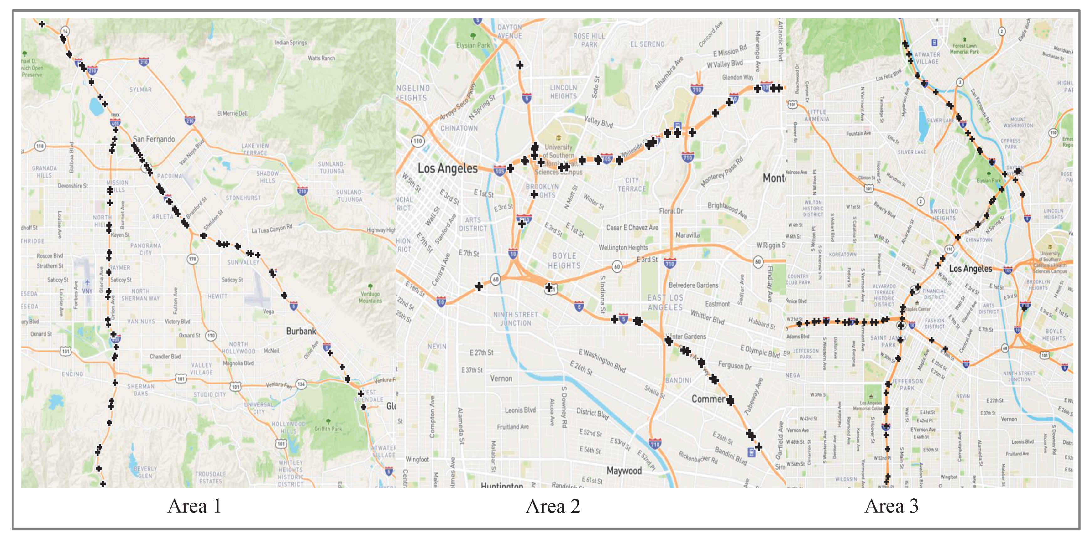
For what concerns the road classification and the levels of traffic flows associated with each road type, it is intuitive that principal or minor arterials may not be as attractive as collectors or distributors. However, in consolidated areas, local roads with commercial land use with various density can be attractors or generators of traffic flows. In such cases, mobility demand can be detrimental to traffic congestions at rush-hour times. To this end, in our case study, three different areas have been selected to illustrate the application of the mD-Resilience approach. The functionality of the area and land use have been obtained from General Plan Land Use (GPLU), which is the fundamental land use policy document of the City of Los Angeles. The dominant land use in area 1 is low-density residential blocks, area 2 is the manufacturing area, and area 3 is the commercial and high-density residential zones, as shown in Figure 5.

Data sources and KPI identification: Traffic flow data used for empirical assessments is from the Caltrans PeMS [48]. PeMS gets its data from Intelligent Transportation System (ITS), traffic counters, Vehicle Detector Stations (VDS), and other sources, such as California Highway Patrol (CHP) incident data, the Caltrans Photolog, etc. Caltrans PeMS consists of 18,300 detector stations and collects traffic data every 30 seconds. Various detailed traffic data are available, such as volume, speed, delay, Vehicle Miles Traveled (VMT), Vehicle Hours Traveled (VHT), travel time, vehicle occupancy, flow, and annual average daily traffic (AADT). Among these data items, speed, volume (flow), and occupancy are measured directly, and other quantities are calculated. PeMS uses postmiles to measure locations on state freeways. In our study, road sections are referring to the sections of roads with functioning measurement stations. We used 5-min traffic flow data of October and November 2018 from major freeways in Los Angeles (i.e., I-10, I-5, I-110, and I-405) for the three identified areas.

In identifying a KPI for performance curve formation and characterization, speed and flow were considered as the preliminary indicators to characterize the macroscopic behavior of roadways. When compared to flow, as also stated in the literature [49], the average speed is a more reliable representative of roadways performance, and it has a closer indication of the behavior of resilience curves. Flow, on the other hand, is noisy and is not consistent with the resilience curve for most cases. Furthermore, based on the fundamental diagram of traffic flow, similar values of flow may correspond to different densities and traffic states (i.e., congested or un-congested regimes) [50].

In order to focus on the recurrent disruptions, we have excluded the data for the weekends given their different traffic patterns (as shown in Figure 6) and, as a common method in the analysis of traffic data, treated weekdays versus weekends separately. Moreover, two criteria were used to separate recurrent congestion (RC) events. RC refers to congestions in the morning or afternoon peak time with a daily pattern. Regular commuters and traffic operators are aware of the duration and location of RC events. They are formed due to excessive travel demand, insufficient traffic capacity, or poor signal control [51]. Since Recurrent congestions are the congestion occurring in morning or afternoon peak times, the first consideration for separating these types of events is to exclude the events that occurred at any time other than morning and evening peak times. Non-recurrent events are due to unexpected events, such as traffic accidents and vehicle breakdowns, or planned events like construction works or inclement weather [52], which may happen in the morning or evening peak times. This may cause a temporal or spatial overlap with recurrent congestions. As such, we used the California Highway Patrol (CHP) historical incident data available at PeMS to identify the overlaps between recurrent and non-recurrent congestions. We excluded the detected events that have temporal and spatial overlap with non-recurrent congestions.

4.2. Resilience Quantification and Interpretation

The mD-Resilience scores were calculated and compared in three different areas with different functionalities and land use. The comparison of the resilience score across different spatial scales and the impact of change in the scale is not in the scope of this study. Our analyses in the case study were centered around the following objectives:

• Evaluating the information gain by using the proposed mD-Resilience approach in a comparative assessment of resilience scores across different areas.
• Understanding how mD-Resilince scores could be used in comparison to conventional metrics of congestion assessment—i.e., delay and bottleneck severity.
• Investigating the impact of different stages of resilience on the response of roadways to recurrent congestions.

With the average speed of the road sections retrieved from PeMS, the congestion events were identified by using a Robustness Range of 10% of free-flow speed according to PeMS definition [48] (i.e., 60 MPH). That means, if the speed drops below 54 MPH, a congestion event occurs, and it is not called recovered until the speed becomes more than 54 MPH. The resilience attributes were calculated by using Equations (3) to (12). In the DEA implementation, we had two input and three output variables, 248 DMUs, and more than 12,000 congestion events (i.e., observations). Therefore, our implementation meets the rule of thumbs for the DEA approach (see e.g., [53]). The total number of inputs and outputs is far less than the number of observations, and the number of DMUs is considerably higher than the sum and multiplication of the numbers of inputs and outputs.

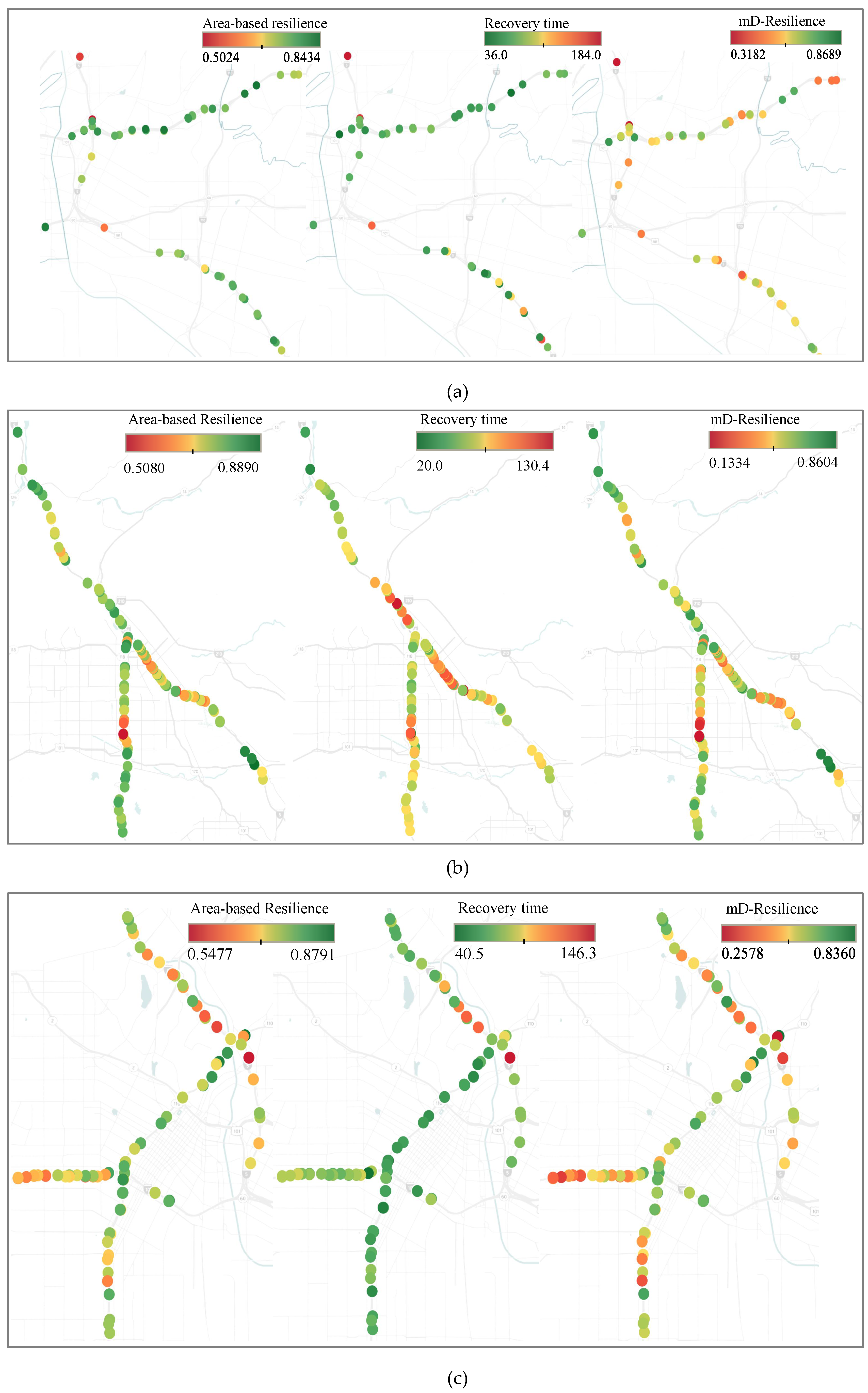
By using the Tableau software application, Figure 7 presents aggregated mD-Resilience scores for different areas in our case study. The same software has been used for visualization of all the geospatial data. Road sections with lower resilience scores are sections that should be further investigated and could be prioritized for remedial actions. Road sections with values closer to one demonstrate a higher resilience against recurrent congestions. As Figure 7 shows, a spatial visualization of the mD-Resilience scores could be used as a tool for comparative assessment. It can be seen that some areas in the network exhibit similar resilience scores. However, a deeper assessment of the individual attributes shows that similar resilience scores may be due to different resilience dimensions. That is, it may be a loss in performance in one section and offsetting the congestion by a long recovery time in another section that resulted in similar resilience scores.

Table 2. The normalized quantified results for three road sections with different levels of resilience.

Station	mD-Resilience Score	Resistance	Loss Rate	Recovery Rate	Event Duration	Recovery Percentage
I-405 S Postmile 65.25	0.133	0.278	0.898	0.330	0.894	0.309
I-5 N Postmile 130.983	0.478	0.578	0.952	0.530	0.968	0.471
I-5 N Postmile 145.03	0.804	0.786	0.963	0.437	0.848	0.507

presents the individual resilience attributes with the corresponding mD-Resilience score for three different road sections. The following discussions provide a more detailed investigation into the impact of multi-dimensional assessment of resilience.

4.2.1. Analysis of Variance

To determine whether there are any statistically significant differences between resilience, delay, and bottleneck metrics, we used the Analysis of Variance for three measures in the case study. Delay values are often considered as a consequence of congestions, and are used to indicate the performance of roadways and transportation serviceability. Bottlenecks cause delays and restrictions in the normal flow of transportation. Bottlenecks are often caused by physical conditions, the design of roads, badly timed traffic signals, or sharp curves. In PeMS, bottlenecks are characterized by four different features, including the number of days active, the average duration, the average extent (in miles), and the average delay. To aggregate these features into one indicator, we used the DEA to quantify the severity (efficiency) of bottlenecks. As mentioned before, in DEA models, desirable variables are output variables (a more efficient system will have higher output values) and input variables are the undesirable ones. Hence, for bottlenecks, all the variables are considered to be the input. An efficiency score between 0 and 1 is assigned to the locations of the bottleneck, with 0 being the worst score. For stations that were not identified as a bottleneck for the period of the study, we have assigned a dummy score greater than 1 to identify them as non-bottleneck stations.

Since distributions of delay and bottleneck scores did not follow a normal distribution pattern, we used the non-parametric statistical test of Kruskal–Wallis H-test for analysis of variance. The p-value resulting from testing these three groups was less than 0.01, demonstrating that the Null Hypothesis has been rejected and that there are significant differences between the distributions of these three metrics. This observation demonstrates how these three performance assessment methods differ in characterizing the performance of the roadways in both concepts and values and could be used as complementary metrics in the assessment.

4.2.2. Comparison with Conventional Resilience Metrics

As noted, the common approach in the quantification of resilience for transportation systems uses the response curve to characterize the varying level of functionality over time. The response curve (sometimes called resilience triangle) consists of three edges and characterize three stages of performance evolution: First, it is the decrease in functionality, second, the recovery time, and the third edge showing the recovery speed. Metrics have been defined based on the resilience triangle to represent the functionality of a system. The area under the resilience curve as the resilience loss due to a disturbance [8,49,54], optimal resilience cost (OR) [55], recovery-dependent resilience (RDR) [55], and recovery time [56] are among metrics usually employed to characterize the resilience of a system. Among these factors, the area-based resilience index and recovery time (or rapidity) are similar in nature to our proposed mD-Resilience score. Area-based resilience index is defined as follows:

$$R=\frac{{\int }_{t_s}^{t_f}P\left(t\right)dt}{\left(t_f-t_s\right)}$$

(15)

The s and f demote start and finish of an event. This index is a scalar value varying between 0 and 1 (1 is the highest resilience level). The recovery time is the duration needed for a full recovery to the final performance that satisfies the overall demand [8,57]. A visual comparison of three resilience indicators is shown in Figure 8. The mD-Resilience scores in most of the road sections show a similar characterization with at least one of the other indicators although in some cases they appear to be more distinctive in differentiating the resilient behavior. An example comparison is seen in

Table 3. Comparison of mD-Resilience scores with recovery time and area-based resilience indices.

Station	mD-Resilience Score	Area-Based Resilience Index	Recovery Time (Minutes)	Level of Service Distribution (Average Daily Hours)	Av. Sum of Flow by Hour (veh/hr)
I-405 S Postmile 65.25	0.133	0.508	110		70,948
I-5 N Postmile 130.983	0.478	0.748	110		100,878
I-5 N Postmile 145.03	0.804	0.858	77		117,187

for three stations (same stations in Table 2) whose physical characteristics are shown in

Table 4. Characteristics of road sections for the stations presented in Table 3.

Station	Number of Lanes	Functional Class	Lane Width (ft)	Latitude	Longitude
I-405 S Postmile 65.25	4	Principal Arterial	11.2	34.188	−118.474
I-5 N Postmile 130.983	4	Principal Arterial	11.3	34.020	−118.181
I-5 N Postmile 145.03	4	Principal Arterial	12	34.170	−118.303

. For station 65.25 of I-405 S, where mD score is 0.133 (relatively low resilience score), recovery time shows significant weakness (110 minutes where maximum observed value is 134) while area-based metric shows a relatively medium resilience. On the other hand, for station 130.983 of I-5 N with a medium mD score, the recovery time shows a low performance, while the area-based metric is relatively high. Moreover, for station 145.03 of I-5 N, where mD score is high, the area-based score is also high, while the recovery time shows a relatively low performance. These observations show that the mD score could provide higher information gain in analyzing the response of roadway sections to disruptions.

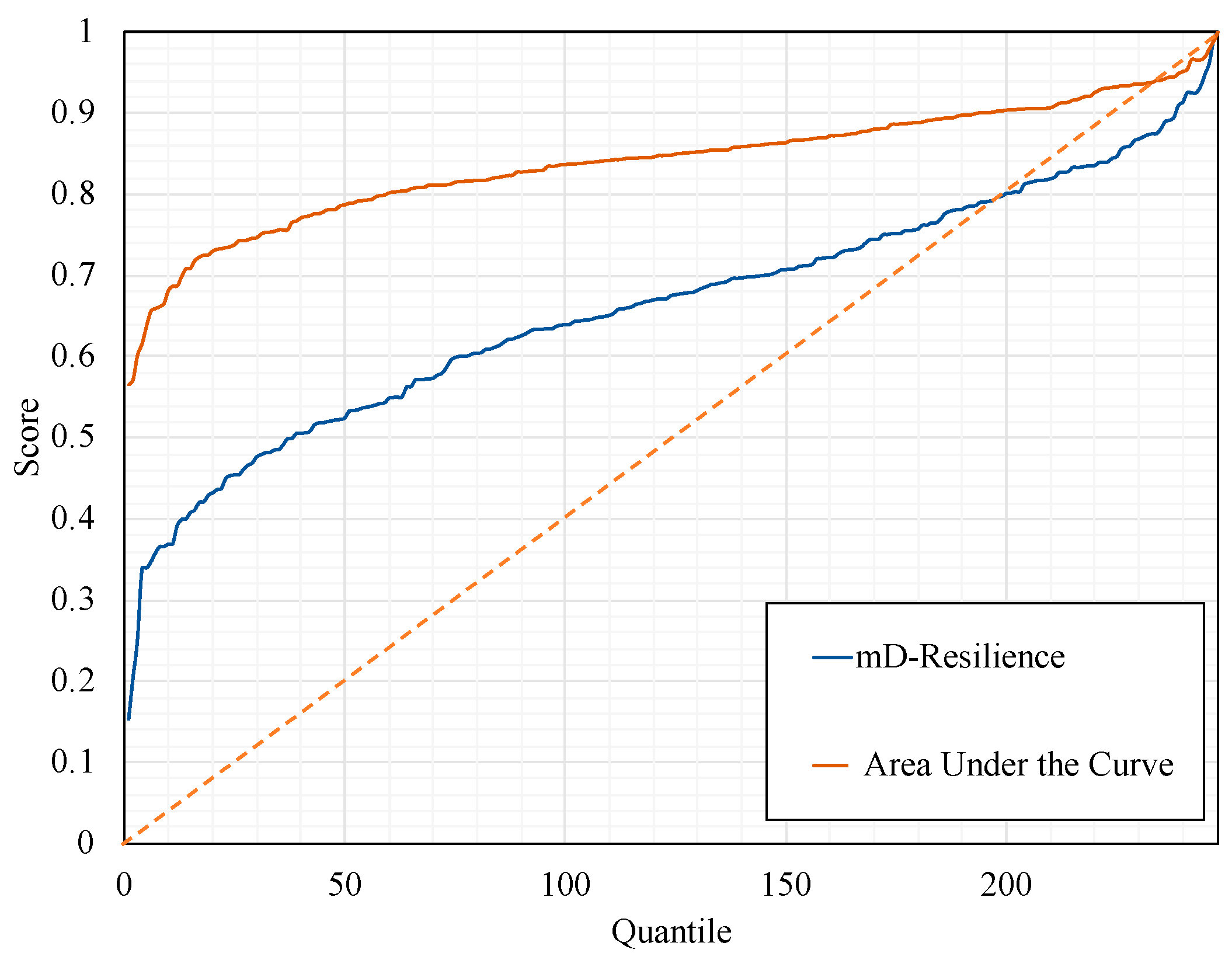
In addition to the qualitative assessment of information gain, a quantitative comparison of area-based resilience characterization and mD score is presented in Figure 9 and

Table 5. Comparison of normalized percentile values of different resilience indicators for the road sections in the case study.

Approach	10th	25th	50th	75th	90th	G* Coefficient	Entropy
Area-based resilience	0.74	0.8	0.84	0.89	0.93	83.61	53.26
mD-Resilience score	0.44	0.55	0.67	0.78	0.84	39.58	74.88

* The area between curves in Figure 9 and the 45° line.

. In doing so, we have normalized the mD scores and area-based resilience scores for all 248 road sections in the area of study between 0 and 1 (using min-max normalization) for better comparison and interpretation. As shown by a Spearman correlation coefficient of 0.87, these two indicators are strongly correlated. However, as it could be seen in Figure 9, the proposed mD-score amplifies the scale to better differentiate road sections with high and low resilience. In other words, it provides more information in distinguishing between the performance of different roadway sections. Table 5 shows the increase in variance as well. For instance, while the 10th percentile of the area-based resilience value is 0.74, the 10th percentile value of the mD score is 0.44. On the other hand, area-based resilience values do not show much variation after the 25th percentile, while mD score smoothly describes the level of resilience and performance of the road sections.

We further quantified the information gain by adopting a concept similar to the Gini coefficient (called it G coefficient) calculation from the Lorenz curve, as well as entropy, to characterize the disparity and distribution of each indicator as shown in Table 5. Borrowing from the concept of the Gini coefficient, in the first step, we compared the difference between the area between the curves in Figure 9 and the 45° line. A smaller area shows a better distribution and higher variability. The mD score shows a value of 39.58, compared to 83.61 for area-based resilience. We further used the sum of entropy for all the stations as representative of information gain. The higher entropy of mD score demonstrates the higher information gain from its use in performance assessment. As shown in Table 5, the mD-Resilience score has led to higher entropy.

4.2.3. mD-Resilience Score and Conventional Performance Metrics

To further reflect on the information gain from mD score and understand its relationship with conventional performance assessment metrics, we investigated how it could be used to infer the categorical severities of delay and bottleneck (high, medium, or low intensity) through decision tree classifiers. This method helps calculate the feature importance as an estimate of the information gain from each individual resilience dimension. Feature importance provides a score that indicates how valuable each feature is in shaping the decision tree to make key decisions in explaining the labels. In this setup, each data point is represented as a vector of individual resilience dimensions. The output is an intensity label obtained from normalized delay and bottleneck score (calculated from DEA) values classified into three groups of low, medium, and high. In training the decision trees, we used all data points that were obtained across three areas of study combined.

Delay and bottlenecks often have been introduced as consequences of traffic congestion. While delay could primarily be due to too much traffic volume, it could also be expected at well-known geographic bottlenecks. It is widely accepted that delay, which may result in late arrival of the users, is an outcome of bottlenecks and traffic congestion. Due to the importance of bottlenecks and delays, we use these two metrics to build the decision-tree classifiers. Two classifiers were built to predict different classes of bottleneck and delay severities based on the resilience dimensions with F-scores of 0.61 and 0.88, respectively. The confusion matrices of these two predictors are as demonstrated in Figure 10. These matrices compare the outcome of the decision tree model on the Y-axis versus the actual classes on the X-axis and provide an overview of the model performance per class. For example, in the case of the delay classifier, 98% of the stations in the class of “high” delay have been correctly identified, while the remaining 2% have been classified as “low” class of delay (top row of delay confusion matrix). As depicted by these matrices, the decision tree for delay prediction has a better performance across all classes, compared to the model for bottleneck severity.

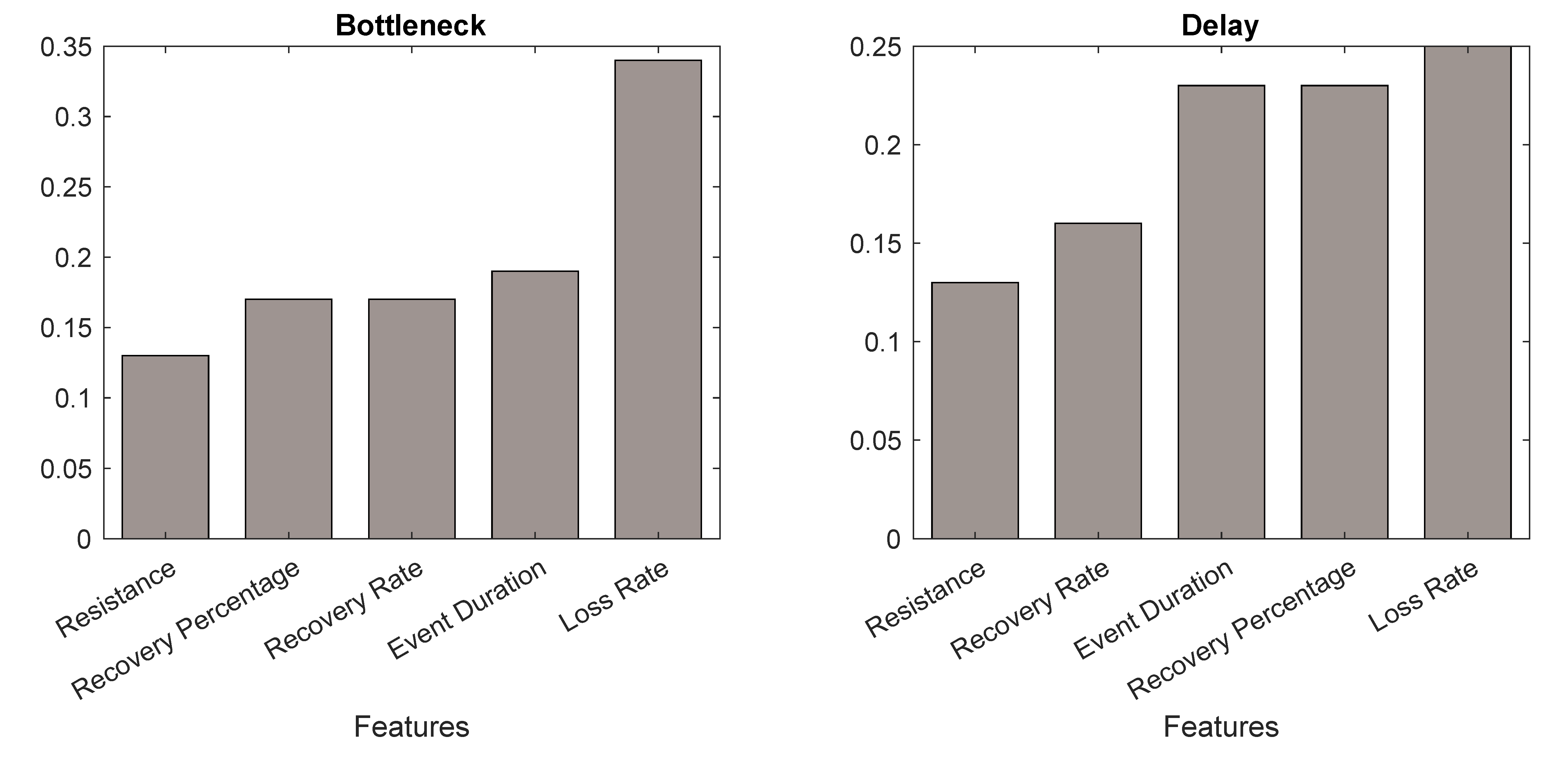
Furthermore, Figure 11 shows the feature importance for both classifiers. From the results, it is clear that all the features play a role in classifying bottlenecks and delays. This suggests that all five proposed dimensions are necessary to describe the performance of a roadway section. This set of analyses shows that the mD dimensions could be used to infer the severity of other conventional performance metrics in addition to providing a new layer of information for performance assessment.

4.2.4. Relationship between Performance and Resilience

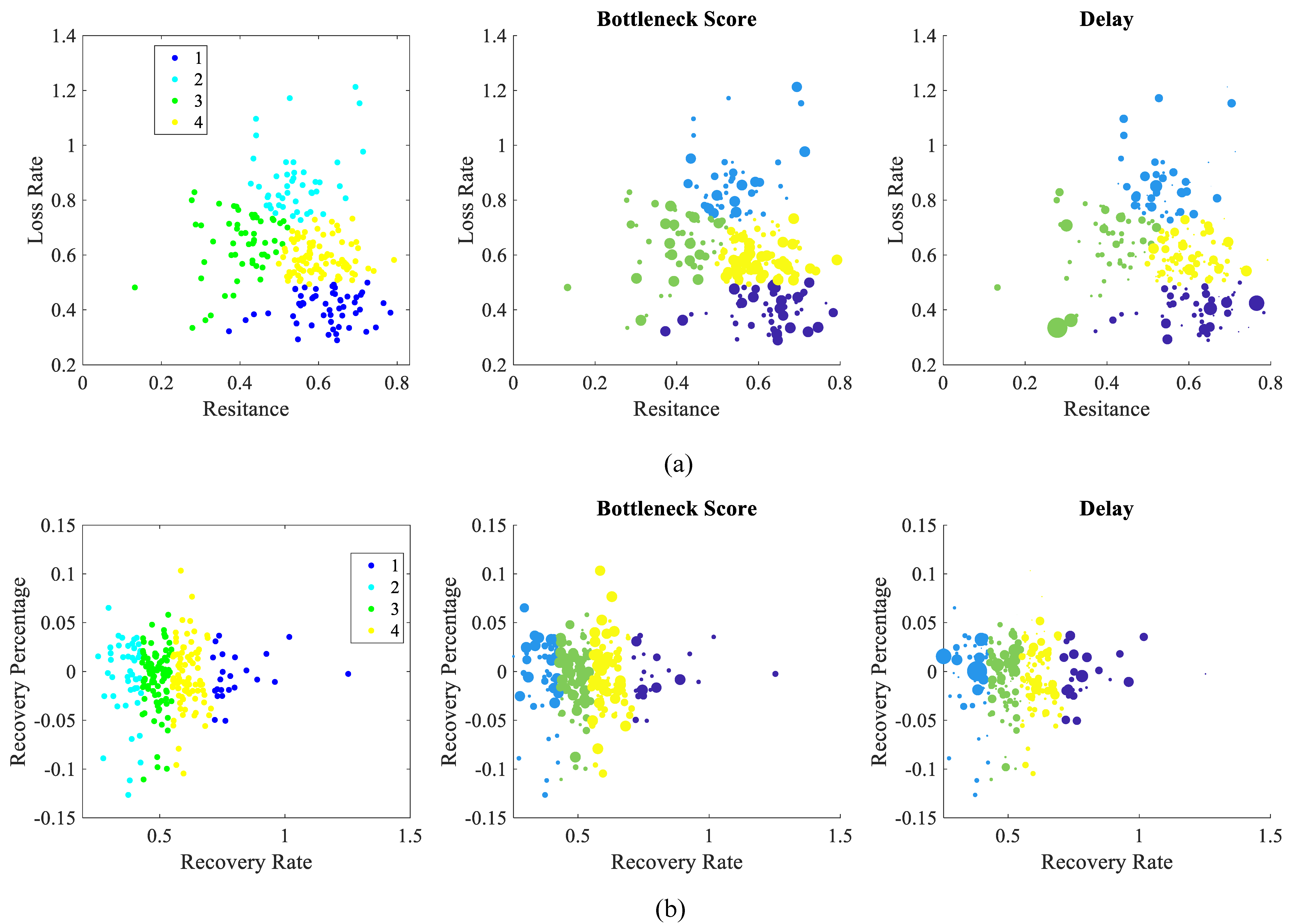
We further investigated the relationship between different severity levels of delay and bottlenecks versus different stages of resilience. To evaluate the sensitivity of bottlenecks and delay values to each stage of resilience (i.e., loss/degradation stage and recovery stage), we performed a clustering analysis for attribute associated with each stage of resilience. In other words, we aimed to examine how loss or recovery characteristics of roadways contribute to characterizing delay and bottleneck severity, and whether we could use them as actionable information. Loss rate and resistance attributes were selected as representative of the loss stage (i.e., before recovery begins). Recovery rate and recovery percentage, on the other hand, were selected as indicators of the recovery stage. The result of K-means clustering (K=4) for loss and recovery stages is as presented in Figure 12a,b, respectively, and on its left column. The data points in the clusters represent the road sections. The average delay and bottleneck score values for the points in each cluster are as shown in Figure 12 on the right side. From a visual assessment of the graphs, it appears that delay is more sensitive to different parameters of resilience stages given the noticeable higher variance across clusters.

Table 6. Impact of resilience measures across loss stage, for delay and bottleneck score.

Cluster Labels	Resistance	Loss Rate	Bottleneck Score *		Delay
			Mean	SD	Mean	SD
2	0.6	0.4	0.55	0.41	32.1	51.33
4	0.6	0.59	0.54	0.4	21.05	22.15
3	0.41	0.66	0.5	0.37	21.57	20.73
1	0.54	0.87	0.44	0.36	33.53	26.86

* Higher scores mean lower severity for the bottleneck.

and

Table 7. Impact of resilience measures across recovery stage, for the delay and bottleneck scores.

Cluster Labels	Recovery Rate	Recovery Percentage	Bottleneck Score *		Delay
			Mean	SD	Mean	SD
4	0.4	−0.05	0.55	0.39	28.02	46.95
1	0.54	−0.08	0.53	0.4	20.65	21.36
3	0.67	−0.01	0.45	0.37	32.12	25.82
2	0.98	0.06	0.36	0.37	36.74	27.62

* Higher scores mean lower severity for the bottleneck.

show key statistics of the delay values and bottleneck scores within each cluster for quantitative assessment with respect to loss and recovery stages, respectively (sorted based on one of the parameters). As these tables show, no special trends could be identified in these tables except for the correlation between the loss rate and severity of bottlenecks in Table 6—higher loss rates have resulted in increased bottleneck severities (lower values). This is another evidence that confirms the observations in Figure 11 demonstrating the importance of all dimensions in characterizing delay and bottleneck events and the fact that different combinations of these two stages could lead to a similar outcome. Furthermore, this analysis shows that we cannot identify ranges of loss or recovery parameters that define an expected resilience outcome as a generic rule.

Kruskal–Wallis H-test was also used to analyze the difference among four clusters of roadways for the loss and recovery stages shown in

Table 8. Kruskal–Wallis test results for delay and bottleneck scores within clusters of resilience stages.

Clustering Feature	Delay		Bottleneck Score
	$\mathbf{Kruskal}’\mathbf{s}\mathit{H}$	$\mathit{p}-\mathrm{Value}$	$\mathbf{Kruskal}’\mathbf{s}\mathit{H}$	$\mathit{p}-\mathrm{Value}$
Loss Stage	8.303	0.016 *	8.659	0.013 *
Recovery Stage	15.380	0.000 *	4.138	0.126

* p < 0.05.

. The $p$-value resulting from testing the groups of delays for both stages of loss and recovery are less than 0.05, demonstrating significant differences between the measurement at the stations when they are grouped based on the loss stage and recovery stage attributes. On the other hand, the $p$-value resulting from testing the groups of bottleneck scores are 0.013 and 0.126, respectively. This suggests that there are significant differences among the bottleneck scores of roadways (at stations) when grouped based on the loss stage attributes ($p<0.05)$, but there is no significant difference that could be inferred when they are grouped by recovery stage attributes. This implies that the delay values could be associated with both the recovery stage and loss stage, while characterizing bottlenecks loss stage attributes could be indicative of the intensity of bottlenecks more distinctly. This is compatible with the observations from Figure 11.

5. Discussion

Given the multi-dimensional nature of the resilience concept for characterizing the performance of roadways and transportation systems, our proposed approach supports combining multiple attributes of resilience into one dimensionless measure, while still providing information on individual stages of resilience. This approach also accounts for novel attributes of “recovery percentage” and “multi-event resilience” to take the recovery paths and partial recovery into consideration. The resilience score is calculated as a relative measure to rank the roadway sections according to their performance as a supplementary metric compared to conventional performance assessment metrics. The research efforts that have used resilience for performance assessment of congestion events have also argued that the use of resilience concept in the quantification of performance has resulted in added information to conventional metrics, such as the delay in travel time [7] and relative congestion index (RCI) [25], which measures the ratio of travel time in congestion to free flow. The increase in the information gain enables a better distinction between different decision-making units (i.e., road sections) for planning purposes. One of the primary advantages of the mD score is that it allows the decision-makers to better understand the relative importance of each attribute for sections with similar resilience scores. Such information may also be used by local authorities for planning resource allocation either for mitigation of loss in performance or for the acceleration of the recovery process.

It should be also noted that the proposed mD-Resilience quantification framework could be applied for performance assessment of systems with different scales, as it uses features from resilience/performance curves of a decision-making unit. For any disruptive event, if a representative key performance indicator (KPI) could be used to form the performance curve and represent system degradation and recovery with sufficient resolution, the mD-Resilience framework and scoring could be applied assuming satisfactory conditions for DEA utilization. However, in this study, we have only presented the performance assessment of roadway sections (as the spatial units) and for the HPLI events considering our motivation and case study. In doing so, we looked at the relatively high-resolution traffic speed data as the KPI and calculated the resilience metrics and their collective impact to quantify the resilience scores. Therefore, the applicability assessment of the framework for other problem domains has remained for future studies. Factors that could influence the outcome of the analysis include data availability and resolution, and the scale of the data analysis (both spatial and temporal). The temporal resolution of the data could change the detected events, the finish time of the event, and as a result, change the values of recovery-related metrics. We have used the average speed of the vehicles (at 5-minute intervals) collected from the stations installed on the freeways. However, the results may differ depending on data availability and type. For example, low-resolution GPS data or other types of onboard mobile sensors could change the representation of the performance curves. In future directions of this research, case studies with various levels of temporal and spatial scales should be taken into account to investigate how these factors change the formation of performance curves and the extraction of resilience attributes. Such investigations will shed light on the data requirements for using the mD-Resilience framework.

The proposed approach reveals the resilience of different sections as symptoms of problems and does not necessarily provide information on potential spatial dependencies in a network. Although this metric provides information on the resistance and recovery stages in coping with a disturbance, causality inference calls for an understanding of the spatial dependencies. Physical and operational characteristics of roadway networks and their impact on upstream and downstream flow in roadways are important in understanding these casualties. However, unlike conventional performance metrics that only identify the severity of the problem, by using the proposed mD-Resilience scoring framework, further information on the coping mechanisms could be identified. Identifying the spatial autocorrelation and propagation of the disturbance waves due to bottlenecks by using data-driven analysis, mathematical modeling, or simulations of road networks are required to infer the causality of observed resilience on the roadway sections.

In this study, we used BCC DEA method, and therefore the evaluations across different DMUs (i.e., road sections) are relative. Other alterations of DEA, such as pairwise comparison, could be further added to enhance the analysis and rank the DMUs with an absolute scale when there is a similar DEA score for multiple DMUs. Furthermore, in real-world situations, different road sections operate in different environments. While we sought to address this by taking the land use classification into account, contextual variables such as road layouts (i.e., the number of lanes, width of roadways, existence of on-ramp and off-ramp, and High Occupancy Vehicle (HOV) lanes) could contribute to the operational conditions and resilience of roadways. This type of information could be added to DEA as the environmental variables, which are often the variables over which the decision-makers have little or no control and are regressed on efficiency scores.

6. Conclusions and Future Work

In this study, a multi-dimensional resilience quantification framework (mD-Resilience) was proposed and evaluated for assessment of the road sections resilience to recurrent (daily based) congestions as a case study. The methodology considers resilience as a complex concept that cannot be fully described by a single feature. Instead, it simulates resilience as the efficiency of a decision-making unit (DMU) (i.e., road sections in our case study) with multiple inputs (representing degradation in performance) and output (representing recovery in performance) sets. Data envelopment analysis (DEA) was adopted for aggregating different features that characterize resilience through maximizing the efficiency of DMUs by using loss rate and event duration as input parameters and resistance, recovery rate, and recovery percentage as output parameters. The non-parametric nature of DEA eliminates the use of assumptions for any relationship between the input and the outputs.

The assessment of the mD-Resilience quantification approach was conducted in a case study for 248 freeway sections in Los Angeles, California on the data from the Caltrans Performance Measurement System (PeMS). Through statistical assessments, it was demonstrated that the mD-Resilience quantification approach could provide supplementary information (compared to conventional metrics such as delay) for performance assessment. Furthermore, it was shown that compared to resilience quantification according to the area under the curve, the mD-Resilience approach results in increased information gain in the assessment of the relative performance reflected in increased entropy for scores across a region. Through decision tree classification analysis, it was further shown that the resilience features introduced in this study could be used to characterize the severity of delays and bottlenecks at three levels of low, medium, and high. Furthermore, feature importance assessments showed that all the individual features are important in characterizing the response of roadway sections; therefore, drawing conclusions on the performance of different sections based on the loss stage or recovery stage alone is not feasible. The future directions of this research include understanding the impact of spatiotemporal data resolution, understanding the implications of mD-Resilience on macroscale transport and mobility problems, and investigating the causality analysis and recommender system though spatial autocorrelation analysis and congestion propagation modeling.

References

1. Calvert, S.C.; Snelder, M. Influence of Weather on Traffic Flow: An Extensive Stochastic Multi-Effect Capacity and Demand Analysis; Institute for Transport Studies in the European Economic Integration: Trieste, Italy, 2016. [Google Scholar]
2. Sarvi, M. Freeway weaving phenomena observed during congested traffic. Transportmetr. A Transp. Sci. 2013, 9, 299–315. [Google Scholar] [CrossRef]
3. Wu, N. A Stochastic Model for Reliability Analysis in Freeway Networks. Procedia Soc. Behav. Sci. 2013, 96, 2823–2834. [Google Scholar] [CrossRef] [Green Version]
4. Murray-Tuite, P.M. A comparison of transportation network resilience under simulated system optimum and user equilibrium conditions. In Proceedings of the 2006 Winter Simulation Conference, Monterey, CA, USA, 3–6 December 2006; IEEE: Piscataway, NJ, USA, 2006; pp. 1398–1405. [Google Scholar]
5. Litman, T. Transportation Cost and Benefit Analysis: Techniques, Estimates and Implications; Victoria Transport Policy Institute: Victoria, BC, Canada, 2009. [Google Scholar]
6. Cox, A.; Prager, F.; Rose, A. Transportation security and the role of resilience: A foundation for operational metrics. Transp. Policy 2011, 18, 307–317. [Google Scholar] [CrossRef]
7. Calvert, S.C.; Snelder, M. A methodology for road traffic resilience analysis and review of related concepts. Transportmetr. Transportmetr. A Transp. Sci. 2018, 14, 130–154. [Google Scholar] [CrossRef]
8. Bruneau, M.; Chang, S.E.; Eguchi, R.T.; Lee, G.C.; O’Rourke, T.D.; Reinhorn, A.M.; Shinozuka, M.; Tierney, K.; Wallace, W.A.; von Winterfeldt, D. A framework to quantitatively assess and enhance the seismic resilience of communities. Earthq. Spectra 2003, 19, 733–752. [Google Scholar] [CrossRef] [Green Version]
9. Rao, A.M.; Rao, K.R. Measuring urban traffic congestion—A review. Int. J. Traffic Transp. Eng. 2012, 2, 286–305. [Google Scholar]
10. de Luca, S.; di Pace, R.; Memoli, S.; Pariota, L. Sustainable Traffic Management in an Urban Area: An Integrated Framework for Real-Time Traffic Control and Route Guidance Design. Sustainability 2020, 12, 726. [Google Scholar] [CrossRef] [Green Version]
11. Pattara-Atikom, W.; Pongpaibool, P.; Thajchayapong, S. Estimating road traffic congestion using vehicle velocity. In Proceedings of the 2006 6th International Conference on ITS Telecommunications, Chengdu, China, 21–23 June 2006; IEEE: Piscataway, NJ, USA, 2006. [Google Scholar]
12. Banik, S.; Bullock, D.M.; Vanajakshi, L. Corridor Level Mobility Analysis Using GPS Data. Int. J. Intell. Transp. Syst. Res. 2019, 18, 1–15. [Google Scholar] [CrossRef]
13. Chen, C. Freeway Performance Measurement System (PeMS). Ph.D. Thesis, University of California, Berkeley, CA, USA, 2003. [Google Scholar]
14. Dong, J.; Mahmassani, H.S. Flow breakdown and travel time reliability. Transp. Res. Rec. 2009, 2124, 203–212. [Google Scholar] [CrossRef]
15. Gong, L.; Fan, W. Applying travel-time reliability measures in identifying and ranking recurrent freeway bottlenecks at the network level. J. Transp. Eng. Part A Syst. 2017, 143, 04017042. [Google Scholar] [CrossRef]
16. Jose, R.; Mitra, S. Identifying and classifying highway bottlenecks based on spatial and temporal variation of speed. J. Transp. Eng. Part A Syst. 2018, 144, 04018075. [Google Scholar]
17. Mishra, S.; Tang, L.; Ghader, S.; Mahapatra, S.; Zhang, L. Estimation and valuation of travel time reliability for transportation planning applications. C. Stud. Transp. Policy 2018, 6, 51–62. [Google Scholar] [CrossRef]
18. Cookson, G.; Pishue, B. INRIX Global Traffic Scorecard–Appendices; INRIX Research: Kirkland, DC, USA, 2017. [Google Scholar]
19. Chen, L.; Miller-Hooks, E. Resilience: An indicator of recovery capability in intermodal freight transport. Transp. Sci. 2012, 46, 109–123. [Google Scholar] [CrossRef]
20. Rose, A. Defining and measuring economic resilience to disasters. Disaster Prev. Manag. Int. J. 2004, 13, 307–314. [Google Scholar] [CrossRef]
21. Sun, W.; Bocchini, P.; Davison, B.D. Resilience metrics and measurement methods for transportation infrastructure: The state of the art. Sustain. Resil. Infrastruct. 2018, 1–32. [Google Scholar] [CrossRef]
22. Litman, T. Lessons from Katrina and Rita: What major disasters can teach transportation planners. J. Transp. Eng. 2006, 132, 11–18. [Google Scholar] [CrossRef] [Green Version]
23. Heaslip, K.; Louisell, W.; Collura, J.; Serulle, N.U. A sketch level method for assessing transportation network resiliency to natural disasters and man-made events. In Proceedings of the Transportation Research Board 89th Annual Meeting, Washington, DC, USA, 10–14 January 2010. [Google Scholar]
24. Khaghani, F.; Jazizadeh, F. Resilience in urban transportation: Towards a participatory sensing-based framework. In Proceedings of the 4th ACM International Conference on Systems for Energy-Efficient Built Environments, Delft, The Netherlands, 8–9 November 2017; ACM: New York, NY, USA, 2017. [Google Scholar]
25. Tang, J.; Heinimann, H.R. A resilience-oriented approach for quantitatively assessing recurrent spatial-temporal congestion on urban roads. PLoS ONE 2018, 13, e0190616. [Google Scholar] [CrossRef] [Green Version]
26. Rahimi-Golkhandan, A.; Khaghani, F.; Garvin, M.J.; Jazizadeh, F. Assessing the Relationship between Transportation Diversity and Road Network Congestion Using Participatory-Sensing Data. In Computing in Civil Engineering 2019: Smart Cities, Sustainability, and Resilience; American Society of Civil Engineers: Reston, VA, USA, 2019; pp. 420–427. [Google Scholar]
27. Zhang, L.; Zeng, G.; Li, D.; Huang, H.-J.; Stanley, H.E.; Havlin, S. Scale-free resilience of real traffic jams. Proc. Natl. Acad. Sci. USA 2019, 116, 8673–8678. [Google Scholar] [CrossRef] [Green Version]
28. Faturechi, R.; Miller-Hooks, E. Measuring the performance of transportation infrastructure systems in disasters: A comprehensive review. J. Infrastruct. Syst. 2014, 21, 04014025. [Google Scholar] [CrossRef]
29. Donovan, B.; Work, D.B. Empirically quantifying city-scale transportation system resilience to extreme events. Transp. Res. Part C Emerg. Technol. 2017, 79, 333–346. [Google Scholar] [CrossRef] [Green Version]
30. Werner, S.D.; Taylor, C.E.; Moore, J.; Mander, J.B.; Jernigan, J.B. New developments in seismic risk analysis for highway systems. NIST Spec. Publ. 1998, 931, 319–343. [Google Scholar]
31. do Céu Almeida, M.; Telhado, M.J.; Morais, M.; Barreiro, J.; Lopes, R. Urban Resilience to Flooding: Triangulation of Methods for Hazard Identification in Urban Areas. Sustainability 2020, 12, 2227. [Google Scholar] [CrossRef] [Green Version]
32. Zhou, Y.; Wang, J.; Yang, H. Resilience of transportation systems: Concepts and comprehensive review. IEEE Trans. Intell. Transp. Syst. 2019, 20, 4262–4276. [Google Scholar] [CrossRef]
33. Donovan, B.; Work, D.B. Using coarse GPS data to quantify city-scale transportation system resilience to extreme events. arXiv 2015, arXiv:1507.06011. Available online: https://arxiv.org/abs/1507.06011 (accessed on 21 July 2015).
34. Santos, T.; Silva, M.A.; Fernandes, V.A.; Marsden, G. Resilience and Vulnerability of Public Transportation Fare Systems: The Case of the City of Rio De Janeiro, Brazil. Sustainability 2020, 12, 647. [Google Scholar] [CrossRef] [Green Version]
35. Ganin, A.A.; Kitsak, M.; Marchese, D.; Keisler, J.M.; Seager, T.; Linkov, I. Resilience and efficiency in transportation networks. Sci. Adv. 2017, 3, e1701079. [Google Scholar] [CrossRef] [PubMed] [Green Version]
36. Twumasi-Boakye, R.; Sobanjo, J.O. Resilience of regional transportation networks subjected to hazard-induced bridge damages. J. Transp. Eng. Part A Syst. 2018, 144, 04018062. [Google Scholar] [CrossRef] [Green Version]
37. Liao, T.-Y.; Hu, T.-Y.; Ko, Y.-N. A resilience optimization model for transportation networks under disasters. Nat. Hazards 2018, 93, 469–489. [Google Scholar] [CrossRef]
38. Zobel, W.C.; Baghersad, M. Analytically comparing disaster resilience across multiple dimensions. Soc. Econ. Plan. Sci. 2018. [Google Scholar] [CrossRef]
39. Khaghani, F.; Rahimi-Glokhandan, A.; Jazizadeh, F.; Garvin, M.J. Urban Transportation System Resilience and Diversity Coupling using Large-scale Taxicab GPS Data. In Proceedings of the 6th ACM International Conference on Systems for Energy-Efficient Buildings, Cities, and Transportation, New York, NY, USA, 13–14 November 2019. [Google Scholar]
40. Tamvakis, P.; Xenidis, Y. Comparative evaluation of resilience quantification methods for infrastructure systems. Procedia Soc. Behav. Sci. 2013, 74, 339–348. [Google Scholar] [CrossRef] [Green Version]
41. Yodo, N.; Wang, P. Engineering resilience quantification and system design implications: A literature survey. J. Mech. Des. 2016, 138, 111408. [Google Scholar] [CrossRef] [Green Version]
42. Mumby, P.J.; Chollett, I.; Bozec, Y.-M.; Wolff, N.H. Ecological resilience, robustness and vulnerability: How do these concepts benefit ecosystem management? Curr. Opin. Environ. Sustain. 2014, 7, 22–27. [Google Scholar] [CrossRef]
43. Zobel, C.W.; Khansa, L. Characterizing multi-event disaster resilience. Comput. Oper. Res. 2014, 42, 83–94. [Google Scholar] [CrossRef]
44. Cutter, S.L.; Burton, C.G.; Emrich, C.T. Disaster resilience indicators for benchmarking baseline conditions. J. Homel. Secur. Emerg. Manag. 2010, 7, 51. [Google Scholar] [CrossRef]
45. Charnes, A.; Cooper, W.W.; Rhodes, E. Measuring the efficiency of decision making units. Eur. J. Oper. Res. 1978, 2, 429–444. [Google Scholar] [CrossRef]
46. Banker, R.D.; Charnes, A.; Cooper, W.W. Some models for estimating technical and scale inefficiencies in data envelopment analysis. Manag. Sci. 1984, 30, 1078–1092. [Google Scholar] [CrossRef] [Green Version]
47. Hricko, A. Global Trade Comes Home: Community Impacts of Goods Movement; National Institute of Environmental Health Sciences: Research Triangle Park, NC, USA, 2008.
48. Varaiya, P. The Freeway Performance Measurement System (PeMS) PeMS 9.0 Final Report; California Partners for Advanced Transit and Highways and University of California Highways Research Report UCB-ITS-PRR--25; University of California: Berkeley, CA, USA, 2009. [Google Scholar]
49. Nieves-Melendez, M.E. Traffic-Based Framework for Measuring the Resilience of Ground Transportation Systems under Normal and Extreme Conditions. Ph.D. Thesis, Virginia Tech, Blacksburg, VA, USA, 2017. [Google Scholar]
50. Ashton, W.D. The Theory of Road Traffic Flow; Methuen: London, UK, 1966. [Google Scholar]
51. Han, L.D.; May, A.D. Automatic Detection of Traffic Operational Problems on Urban Arterials; Institute of Transportation Studies, U.C. Berkeley: Berkeley, CA, USA, 1989. [Google Scholar]
52. Kwon, J.; Mauch, M.; Varaiya, P. Components of congestion: Delay from incidents, special events, lane closures, weather, potential ramp metering gain, and excess demand. Transp. Res. Rec. 2006, 1959, 84–91. [Google Scholar] [CrossRef]
53. Cooper, W.W.; Seiford, L.M.; Zhu, J. Handbook on Data Envelopment Analysis; Springer Science & Business Media: Berlin/Heidelberg, Germany, 2011; Volume 164. [Google Scholar]
54. Reed, D.A.; Kapur, K.C.; Christie, R.D. Methodology for assessing the resilience of networked infrastructure. IEEE Syst. J. 2009, 3, 174–180. [Google Scholar] [CrossRef]
55. Vugrin, E.D.; Warren, D.E.; Ehlen, M.A.; Camphouse, R.C. A framework for assessing the resilience of infrastructure and economic systems. In Sustainable and Resilient Critical Infrastructure Systems; Springer: Berlin/Heidelberg, Germany, 2010; pp. 77–116. [Google Scholar]
56. Tierney, K.; Bruneau, M. Conceptualizing and measuring resilience: A key to disaster loss reduction. TR News 2007, 250, 14–17. [Google Scholar]
57. Chang, S.E.; McDaniels, T.; Fox, J.; Dhariwal, R.; Longstaff, H. Toward disaster-resilient cities: Characterizing resilience of infrastructure systems with expert judgments. Risk Anal. 2014, 34, 416–434. [Google Scholar] [CrossRef] [PubMed]
Figure 1. Resilience curves with a similar performance loss area and different behavior.
Sustainability 12 04879 g001
Figure 2. Resilience attributes based on the evolution of performance degradation and recovery.
Sustainability 12 04879 g002
Figure 3. System performance and partial recoveries under multiple disturbances (failure to full recovery).
Sustainability 12 04879 g003
Figure 4. The process of multi-dimensional resilience characterization.
Sustainability 12 04879 g004
Figure 5. Layout of the areas, evaluated in our case study in Los Angeles, California.
Sustainability 12 04879 g005
Figure 6. Speed variation pattern for a typical week in November for a station in I-5 S.
Sustainability 12 04879 g006
Figure 7. mD-Resilience (multi-dimensional resilience) scores for road sections in (a) Area 1 (low-rise residential), (b) Area 2 (Manufacturing), (c) Area 3 (Commercial and high-rise residential).
Sustainability 12 04879 g007
Figure 8. Comparison of three different resilience characterization indicators for (a) Area 1, (b) Area 2, and (c) Area 3.
Sustainability 12 04879 g008
Figure 9. Comparison of different resilience-based performance indicators. Although highly-correlated, the indicators are not one-to-one matched.
Sustainability 12 04879 g009
Figure 10. Confusion matrices in classifying bottleneck and delay categories; X-axis shows actual severity groups and Y-axis shows the predicted severity groups.
Sustainability 12 04879 g010
Figure 11. Feature importance in training decision tree classifiers for bottlenecks and delays.
Sustainability 12 04879 g011
Figure 12. Clustering the stations based on: (a) Loss stage features, (b) recovery stage features.
Sustainability 12 04879 g012