Article

The Study of Gaining More Detailed Variability Information of Soil Organic Carbon in Surface Soils and Its Significance to Enriching the Existing Soil Database

1
School of Geography, Geomatics, and Planning, Jiangsu Normal University, Xuzhou 221116, Jiangsu, China
2
Department of Agricultural Chemistry, National Taiwan University, Taipei 10617, Taiwan
*
Author to whom correspondence should be addressed.
Sustainability 2020, 12(12), 4866; https://doi.org/10.3390/su12124866
Submission received: 8 May 2020 / Revised: 8 June 2020 / Accepted: 11 June 2020 / Published: 15 June 2020
(This article belongs to the Section Sustainable Agriculture)

Abstract

:
To meet the increasing demands of precision agricultural and environmental management, more abundant and accurate information is needed to describe soil organic carbon (SOC) vertical variation. Based on 923 soil profiles (collected at the depths of 0–15, 15–30, 30–60, 60–90, 90–120, and 120–150 cm) in the central area of Changhua County, Taiwan, the distribution curve of the SOC content of each profile was fitted by the equal-area spline model, and it was possible to obtain the SOC content at all depths. Taking the 0–5 cm (L1), 5–10 cm (L2), and 10–15 cm (L3) sub-layers as examples, their SOC contents and stocks were compared to the mean values of the average 5-cm-thick sub-layers (Lm) derived from the value of the 0–15 cm layer. The results indicated that the SOC contents and stocks both reduced with increasing soil depths. The mean SOC contents of L1, L2, and L3 were 22.1, 21.0, and 18.7 g·kg−1, respectively, with significant variation, and the values of L2 and L3 were 5.0% and 15.4% lower than that of L1. Similarly, the mean SOC stocks were 1.29, 1.25, and 1.16 kg·m−2 of the L1, L2, and L3 layers, also with significant variation, and the values of L2 and L3 were 4.0% and 10.1% lower than that of L1. Meanwhile, it was found that the SOC content and stock of Lm were both close to the corresponding values in L2, but were significantly different to that of L1 and L3. Furthermore, the interpolation contours of the SOC contents and stocks in L1, L2, and L3 by digital soil mapping also presented regular variation with increasing soil depths, while the contours of Lm had nearly identical patterns to that of L2. The results demonstrate that the typically used mean SOC contents with certain thicknesses calculated from the sampling layer can only approximately inflect the SOC situation at intermediate depths, but the SOC content in the upper and lower parts within the sampling layer varies greatly. Therefore, the actual distribution of SOC varies gradually depending on the soil depth. This study indicates that the combination of the equal-area spline model and digital soil mapping can greatly enrich the current soil SOC database and provide more abundant and accurate SOC content and stock information for precision agricultural and environmental management based on legacy soil database.

1. Introduction

As an important soil property, soil organic carbon (SOC) is not only a key indicator of soil quality, but also has an important impact on the global carbon cycle [1,2,3]. Due to complicated soil-forming factors and increasing human activities, SOC usually has high spatial variability in the horizontal and lateral directions [4,5,6,7]. At present, with the in-depth study of digital soil mapping and precision agriculture, the variability in the horizontal and lateral directions has become an important research topic for soil researchers [8,9]. More abundant and accurate soil information is needed to describe the characteristics of SOC spatial variation. Hence, investigating the variability characteristics of SOC in more detail is essential for establishing environmental protection and agricultural management measures.
The study of SOC variation in the lateral direction is an important aspect of spatial variability, as well as in the horizontal direction, and some progress has been made in recent years [10,11,12]. Some researchers have studied regional SOC distributions in different sampling layers based on soil profile data. Jacinthe et al. (2011) studied the SOC stocks in the plow layer (0–30 cm) and at a depth of 0–100 cm in the irrigated cotton agro-ecosystems of New Mexico (USA) based on representative multi-layer sampling profiles, and found that the SOC stock at both depths (using organic farming practices) was 37.70 and 76.80 Mg ha−1, respectively [13]. Tsui et al. (2013) predicted SOC stocks from a dataset of 19,024 soil pedons of three soil types from areas in Taiwan; the results indicated that the SOC stock was 2.1–3.8 kg·m−2 at a depth of 0–15 cm and 3.9–6.8 kg·m−2 at a depth of 0–30 cm in the three areas [14]. Previous studies have mainly calculated SOC stocks and mapped their spatial distributions in different sampling soil layers based on the mean SOC values of the corresponding soil layers. Some studies have pointed out that SOC usually continuously varies with different soil depth profiles, as well as with other soil attributes [15,16]. It is difficult to accurately express the continuously varying characteristics of SOC for different sampling layers with the discontinuous SOC values of mixed soil samples. Therefore, it is necessary to develop a method to modify horizon data in order to make it more continuous. In the 1940s, a first attempt was made by drawing freehand curves along the mid-point depth of various sampling layers with the corresponding soil data [17]. Afterward, more complicated methods appeared in the 1960s–1970s. For instance, Russell and Moore (1968) proposed the exponential decay function for fitting continuous soil attributes with depth [18]. Campbell et al. (1970) and Colwell (1970) developed multi-degree linear regression and polynomials, respectively, for fitting the soil attributes along the profiles [19,20]. To overcome the drawbacks due to the impact of the local variation in soil profiles on the fitting quality, Jauregui and Quirino (1985) used the spline function to fit a smooth independent function over small intervals of the soil profiles [21]. Ponce-Hernandez et al. (1986) proposed an equal-area spline, a variation of the spline function, to model soil attribute depth functions, and found it can obtain a better fitting result [22]. At present, equal-area spline has been fully verified and used widely by soil scientists, and is deemed a practicable method to predict soil attribute data in the random depths of a soil profile [23,24,25]. This makes it possible for us to obtain more abundant and accurate information of SOC at various depths based on the soil profile data.
The topsoil (0–15 cm) is the most active area of SOC variation and accounts for a large proportion of the C pool [26]. Most agricultural productions and an abundance of microorganism activities occur in this layer. The results of several studies have indicated that 69–94% of the roots of most crops are located in the top 10 cm of the soil [26,27,28]. For many crops, their roots in the early growth stages absorb nutrients from the shallow topsoil [29,30]. Nong et al. (2013) found that the root system of wheat mainly absorbs nutrients from soil at a depth of 0–5 cm before the heading stage on the Loess Plateau of China [31]. Moreover, it is well known that soil moisture, air, nutrient conditions, and the microbial species and quantities all vary with different soil depths in the topsoil, and SOC in the top layer also has a certain variability in the lateral direction without exception. The abundance and accuracy of SOC data regarding sub-layers with smaller intervals in topsoil have increasingly practical significance for precision agricultural management and accurate soil mapping. However, there are still few studies that focus on this issue. It is obvious that the existing soil data can hardly meet the realistic demands. For this reason, the present study was initiated in Changhua County in Taiwan with high-density soil sampling points. Based on the SOC variety curves fitted by equal-area spline in every soil profile, the SOC contents and stocks in the 0–5, 5–10, and 10–15 cm sub-layers were predicted and compared to the mean values of the whole topsoil layer (0–15 cm), which is typically used to represent the SOC status at any depth of topsoil. The objectives of this study were: (1) to evaluate the difference between the SOC values of different sub-layers (i.e., 0–5, 5–10, and 10–15 cm) in the topsoil and the average value of the whole soil layer; and (2) to discuss the practical effects of fine soil mapping on agricultural production, and the significance of enriching soil databases with historical soil data and the equal-area spline model. The results provide reference for establishing more proper agricultural measurements and digging processes in order to obtain more accurate soil information.

2. Materials and Methods

2.1. Study Area

This study was conducted in the north of Changhua County (120°15′53” to 120°37′56” E, 23°47′30” to 24°11′40” N), which is located in the central part of Taiwan, between the Choushui River and the Dadu River (Figure 1). The study area, about 83 km2 in size, is located on the south bank of the Dadu River. In this area, the terrain is generally gentle, and the elevation decreases gently from the eastern terrace to the western coastal plain, with a gradient about 1:400. The climate is of a warm and moist southern subtropical type, and the mean air temperature is 17.3 °C in winter and 28.0 °C in summer. The mean annual rainfall is 1733 mm, based on official data from the Central Weather Bureau of Taiwan over the past 30 years (1987–2017). The parent material of soil formation is mainly the alluvial materials, such as sand gravel, sand, and clay, brought by the Dadu River. A difference in parent material has an important effect on the formation of soil types in this area. The major soil type is Shuishui Series (Typic Endoaquept, U.S. Department of Agriculture (USDA), Soil Taxonomy) in the south region of the study area, and Homei Series (Typic Udorthent, USDA Soil Taxonomy) in the north central region. The general characteristics of the Shiushui Series and Homei Series soil types from the soil survey in Changhua County are shown in Table 1 [32]. Paddy rice, vegetables, and fruits are the major crops in the study area.

2.2. Soil Sampling and Laboratory Analysis

Following the Soil Survey Manual [33], the soil sampling program in this study was conducted with arable soils. In total, 923 soil profiles were collected based on regular grids of 250 m × 250 m. Then, the sampling profiles were randomly divided into two parts: 646 profiles, about 70% of the total, were used for fitting the variety curves of the SOC contents and stocks by the equal-area spline model, and for obtaining the spatial interpolation contours of the SOC content and stock in the 0–5 cm (L1), 5–10 cm (L2), and 10–15 cm (L3) sub-layers. The remaining 277 soil profiles, about 30% of the total, were used for validating the spatial interpolation accuracy of the SOC content and stock in the various sub-layers. The entire profiles of the soil samples were all collected from six layers, namely 0–15, 15–30, 30–60, 60–90, 90–120, and 120–150 cm, from 2001 to 2002. The location of every sampling profile was geo-referenced by global positioning system (GPS), and the corresponding pedologic information of each profile was described. After the animal and plant residues had been removed from all soil samples, they were air-dried, ground, and sieved (using a 2-mm 10 mesh), and then the soil organic carbon content was determined by the K2Cr2O7 (0.8 mol/L) oxidation–titration method [34].

2.3. Calculation of the SOC Contents and Stocks

The SOC stock for a given depth in the arable soil is calculated as follows:
S O C   s t o c k   ( kg · m 2 ) = [ S O C   ( g · kg 1 ) × B d   ( g · cm 3 ) × t h i c k n e s s   ( cm ) ] / 100
where B d is the soil bulk density and t h i c k n e s s refers to the thickness of the soil layer [35].
In practical application, the SOC values of sub-layers of any thickness in the sampling layer are usually substituted by the average value of the whole sampling layer. For comparison of the SOC contents and stocks, the three sub-layers of 0–5 (L1), 5–10 (L2), and 10–15 cm (L3) were selected and compared to the sub-layer of a mean thickness of 5 cm (Lm) within the 0–15 cm soil layer. It is noted that the SOC contents and the corresponding soil Bd in L1, L2, and L3 were both fitted and predicted by the equal-area spline model (described in Section 2.4) based on the database of 646 profiles. Then, the SOC stocks in the various sub-layers were calculated by Equation (1). The mean SOC value of every 5-cm-thick sub-layer (Lm) was equivalent to the mean value of the 0–15 cm soil layer. The SOC stock value in Lm was calculated by dividing the total value of the 0–15 cm layer by 3, which is currently the most conventional method to obtain the SOC stock values of certain thicknesses. When comparing the SOC contents and stocks among L1, L2, L3, and Lm, analysis of variance was used for revealing any significant differences.
Although only the SOC contents and stocks in the 0–5, 5–10, and 10–15 cm sub-layers of topsoil were studied in this research, to ensure reliability of the fitting, six soil sampling layers (i.e., 0–15, 15–30, 30–60, 60–90, 90–120, and 120–150 cm) of all profiles were used for the equal-area spline model.

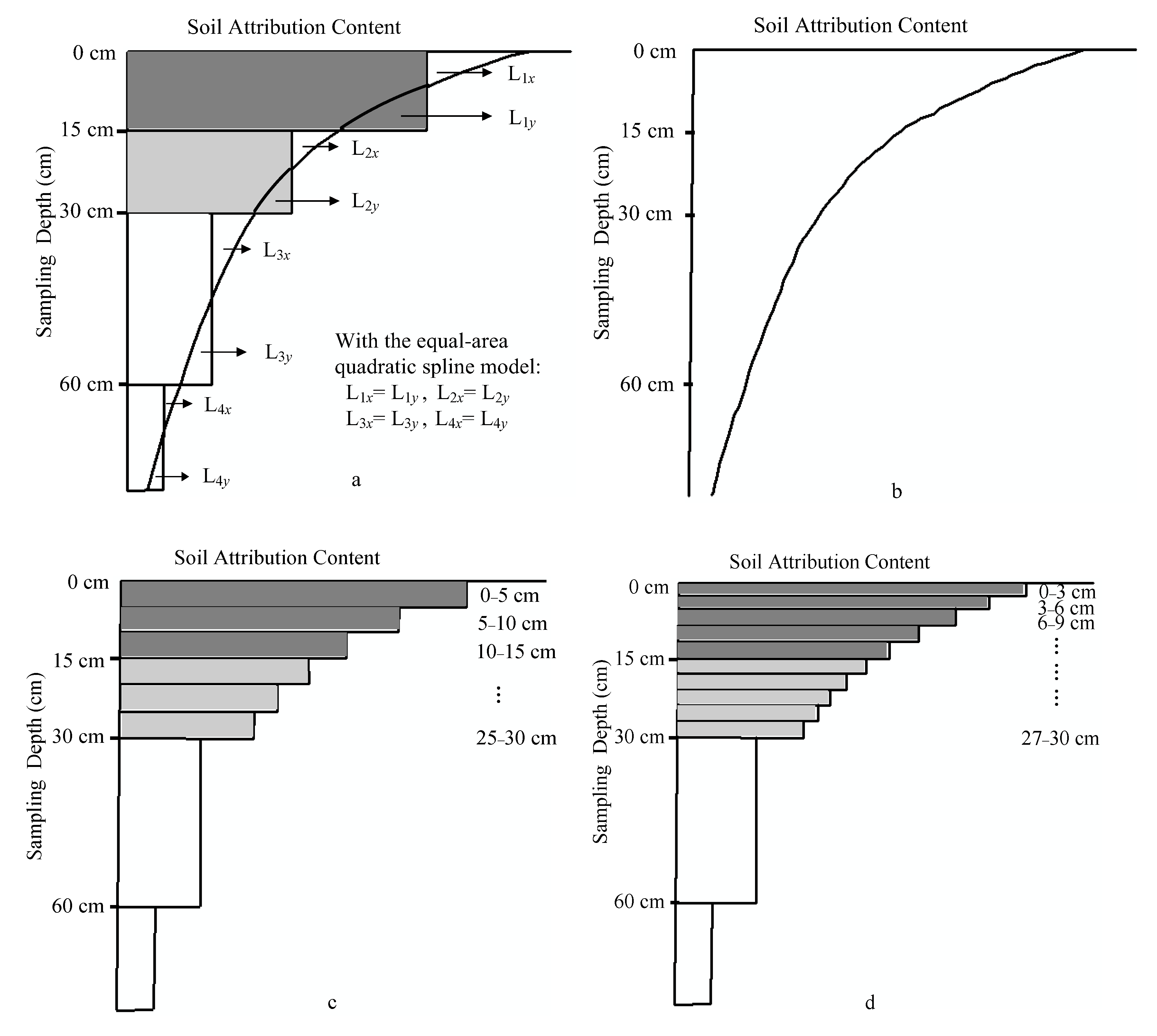
2.4. Calculation of the SOC Contents and Stocks in the Sub-Layers of Topsoil Using the Equal-Area Spline Model

Based on the data of various soil profiles, Bishop et al. (1999) demonstrated the ability of the equal-area spline model to predict soil attribute depths functions by comparing it with other mathematical methods [23]. As the premise of the model, it was assumed that true soil organic carbon values vary smoothly with depth. The soil depth can be denoted by x, and the true attribute values can be described by f(x). As the true SOC values vary smoothly with soil depth, this means f(x) and its first derivative f′(x) are both continuous, and that f′(x) is a square integrable. Assuming that there are n sampling layers in a soil profile, the depths of the boundaries of the n layers can be defined by x0<x1<…<xn; because x0 is the soil surface, x0 = 0. The measurement of the mixed sample from layer i is assumed to reflect the mean attribute level, apart from the measurement error. Mathematically, the measurements are modeled as [23,36]:
y i = f i ¯ + e i
where f i ¯ is the mean value of f(x) over the interval (xi − 1, xi) and ei refers to the measurement errors with a mean of 0 and a variance of σ2. f(x) represents a spline function, which can be found by mini-missing:
1 n i = 1 n ( y i f i ¯ ) 2 + λ x 0 x n f ( x ) 2 d x
The first term represents the fit to the data, while the second term measures the roughness of function f(x), expressed by its first derivative f′(x). Parameter λ controls the trade-off between the fit and the roughness penalty. The solution is a linear–quadratic smoothing spline, i.e., linear between layers and quadratic within layers. The equal-area quadratic splines were fitted using code written in S-PLUS [37], a statistical computer language (Figure 2). In this study, the best λ value was 0.01, in accordance with the results of previous research [11,23].

2.5. Spatial Interpolation and Evaluation of its Accuracy

To obtain spatial distribution maps of the SOC contents and stocks of the sub-layers of 0–5, 5–10, and 10–15 cm within study area, the ordinary kriging method of geostatistics and digital soil mapping techniques were used in this study. Ordinary kriging is able to make a linear optimal unbiased estimation of the value of the regionalized variables of unsampled points by the sampled data [38]. In this method, the spatial patterns of the soil attributes can be described using the following semivariogram model γ(h) (Equation (4)). The principle and interpolation semivariance of the ordinary kriging method have been described in detail in many studies [38,39].
γ ( h ) = 1 2 N ( h ) i = 1 N ( h ) [ z ( x i ) z ( x i + h ) ] 2
where N ( h ) is the number of data pairs separated by a distance h , and z ( x i ) and z ( x i + h ) are the measured values for the regionalized variables z ( x ) at the position of x i and x i + h , respectively.
Kriging is expressed as a linear weighted average of the observations in the neighborhood of the unsampled location x 0 (Equation (5)):
Z ( x 0 ) * = i = 1 n λ i z ( x i )
where Z * ( x 0 ) is the predicted value at location x 0 ; z ( x i ) is the measured value for the soil attribute at position x i ; λ i is the weight of the corresponding measured value obtained from the kriging system; i = 1 n λ i = 1 ; and n is the number of measured samples. In this study, the SOC mapping resolutions of various soil sub-layers were all 15 m.
To evaluate the interpolation accuracy of the SOC contents and stocks by kriging in the 0–5, 5–10, and 10–15 cm sub-layers, the Pearson’s correlation coefficients (r) between the predicted and measured SOC values of the 277 validation samples, as well as the root mean square error (RMSE), were compared (Equation (6)). Larger r and smaller RMSE values indicate higher prediction accuracy.
R M S E = 1 n ( x o i x p i ) 2
where n is the number of validation points, xoi refers to the measured values, and xpi denotes the predicted values by kriging interpolation for the validation points.

2.6. Statistical Analysis Software

The semivariograms of the SOC data were characterized and modeled using the software package GS + 9.0 (Geostatistics for the Environmental Science, Plainwell, MI, USA), and the kriging interpolations were conducted in ArcGIS 9.3 (ESRI Inc., Redlands, CA, USA). The statistical analysis was completed using SPSS 16.0 for Windows (SPSS, Chicago, IL, USA), and the RMSE comparison charts of the SOC contents and stocks were drawn using OriginPro 8.0 (OriginPro 8, OriginLab Corporation, MA, USA).

3. Results

3.1. Mean SOC Contents and Stocks in Every 5-cm-Thick Sub-Layer of Topsoil

Based on the 646 topsoil (0–15 cm) profiles in the study area, the mean SOC content and stock of every 5-cm-thick sub-layer (recorded as Lm) are shown in Table 2. The statistics show that the mean SOC content of the topsoil was 20.5 g·kg−1. The SOC stock in Lm, calculated by Equation (1) with the Bd data (Table 2), was 1.23 kg·m−2. The coefficients of variation (CVs) of the SOC content and stock in Lm were 0.35 and 0.31, respectively, and all values have moderate variability. Judging from the coefficients of skewness, the SOC content and stock in Lm both fit the normal distribution well.

3.2. SOC Contents and Stocks in the 0–5, 5–10, and 10–15 cm Sub-Layers

Fitted by the equal-area spline model, the SOC contents and Bd in the 0–5 (L1), 5–10 (L2), and 10–15 cm (L3) sub-layers were predicted based on all 646 soil profiles (Table 2). The mean SOC contents in L1, L2, and L3 were 22.1, 21.0, and 18.7 g·kg−1, respectively, with the corresponding change ranges of 55.6, 50.7, and 43.7 g·kg−1. The analysis of variance (ANOVA) showed that the mean SOC contents of the three sub-layers were significantly different (p < 0.05). Obviously, the mean contents of the sub-layers decreased continuously as the depth increased, and the contents in L2 and L3 were 5.0% and 15.4% lower than that in L1, respectively. The soil Bd values in the various sub-layers were 1.19, 1.21, and 1.26 g·cm−3, respectively, and increased as the soil depth increased, thus showing an opposite trend to that of the SOC contents. The Bd values in L2 and L3 were 1.7% and 5.4% higher than that of L1.
The SOC stocks in the various sub-layers were calculated from the matching SOC contents and Bd by Equation (1). As Table 2 shows, the SOC stocks were 1.29, 1.25, and 1.16 kg·m−2 in L1, L2, and L3, respectively; the values and the ranges of the SOC stock showed similar trends that both decreased as the soil depth increased. Meanwhile, there were significant differences among the mean SOC stocks in L1, L2, and L3 according to the ANOVA. The SOC stocks in L2 and L3 were 4.0% and 10.1% lower than that in L1, respectively, which were less than the corresponding reductions in SOC content as the Bd increased with soil depth. From the CVs, the variability of the SOC stocks reduced as the soil depth increased, as well as the SOC contents. Furthermore, when comparing to the mean values in the Lm sub-layer, there were significant differences with the SOC contents and stocks in the sub-layers of L1 and L3, while there were no significant differences with the corresponding values in sub-layer L2.

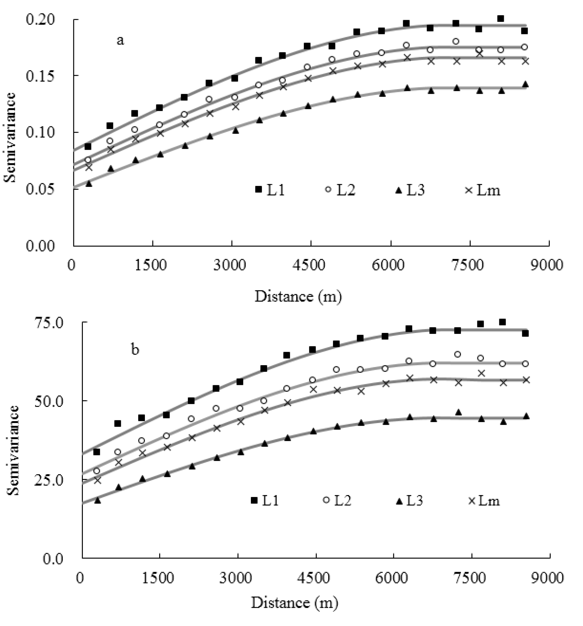
3.3. Geostatistics Analysis of the SOC Contents and Stocks in the Various Sub-Layers

The semivariograms and optimal fitting models of the SOC contents and stocks in the L1, L2, L3, and Lm sub-layers are outlined in Table 3 and Figure 3. It can be observed that the SOC contents and stocks in the various sub-layers showed strong stochastic and structural characteristics. All SOC content and stock data were best fitted by the spherical model. In terms of the nugget to sill ratio (C0/Sill), which represents the degree of spatial dependence, the SOC contents and stocks all had moderate spatial correlation in the various sub-layers. The sill gradually reduced as the depths increased from L1 to L3, while the range had the opposite trend (Figure 3 and Table 3). This result indicates that the variations of the SOC contents and stocks in the surface 0–5 cm sub-layer were larger than those of the lower sub-layers, which is consistent with the variation trend in the CVs of the SOC contents and stocks in L1, L2, and L3 (Table 2). Moreover, the closer to the surface, the more easily SOC is disturbed by local factors, which is what led to the increasing trend in the autocorrelation distance as the soil depth increased. Consequently, the spatial dependency distance of the surface 0–5 cm sub-layer was slightly shorter than that of the deeper sub-layers. Furthermore, the data showed that most of the parameters in the Lm sub-layer were close to the L2 sub-layer, owing to their closely related SOC data.

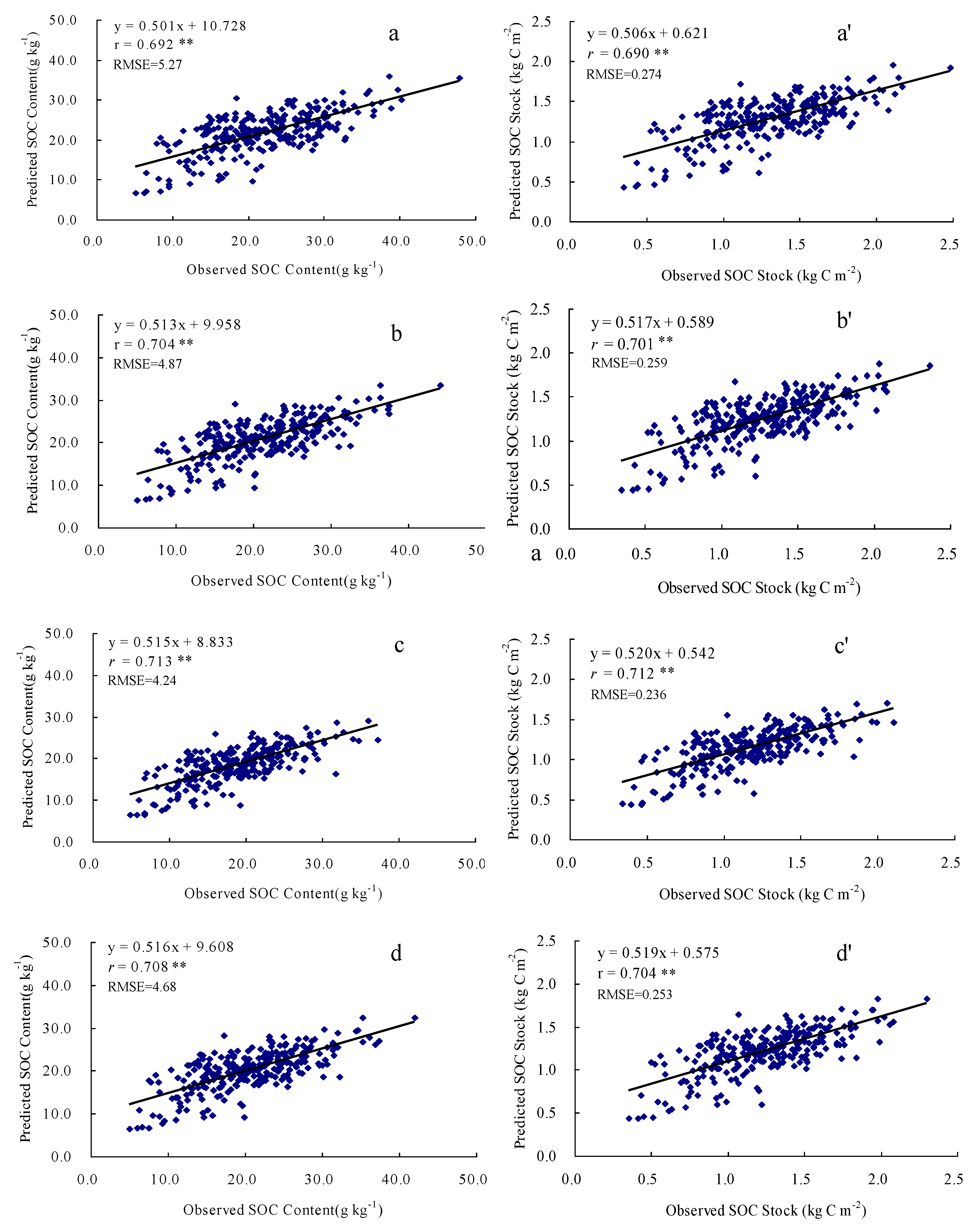
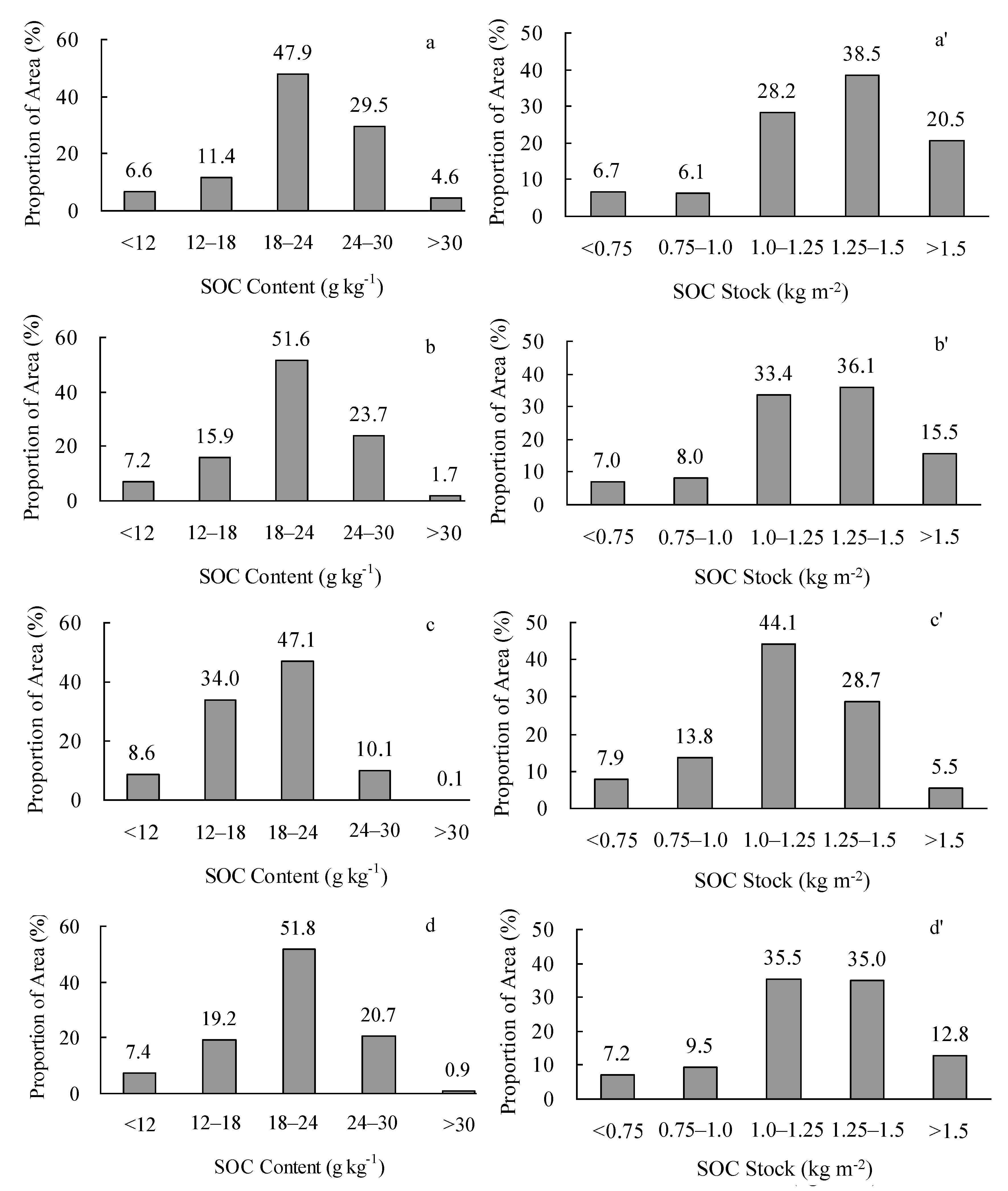
3.4. Interpolation Maps and Accuracy Evaluation of the Various Sub-Layers

Based on the 277 validation sampling points, the interpolation accuracy of the SOC contents and stocks by the kriging method in the various sub-layers is shown in Figure 4. The correlation coefficients (r) between the measured and predicted SOC contents and stocks were all significant (p < 0.01). The rs of the SOC content (r = 0.692) and stock (r = 0.690) in L1 were almost same as those in L2 or L3. As shown in Figure 4, the predicted RMSEs of the SOC contents in the L1, L2, and L3 sub-layers were 5.27, 4.87, and 4.24 g·kg−1, and accounted for 25.7%, 23.8%, and 20.7% of the mean value of the topsoil, respectively. The RMSEs of the SOC stocks of the corresponding layers were 0.274, 0.259, and 0.236 kg·m−2, and accounted for 19.3%, 18.2%, and 16.6% of the mean value of any 5-cm-thick sub-layer in the topsoil, respectively. In general, the interpolation accuracy of the SOC contents and stocks for each sub-layer was acceptable.
The spatial interpolation contours of the SOC contents and stocks in the various sub-layers produced by the kriging method are shown in Figure 5. In the lateral direction, the contours of L1, L2, and L3 show similar distribution patterns. They both had higher SOC contents and stocks in the south region, while lower SOC contents and stocks in the northeastern region. This is because the SOC content and stock are related to land use and the corresponding management measures. In the south region of the study area, the soils are mainly formed by the parent material of viscous slate alluvium. In addition to the better irrigation conditions in this area, land use is dominated by paddy fields. As a result, soil in this region is generally under reduction conditions owing to long-term water flooding, which is conducive to the accumulation of SOC. By contrast, the soils in the north central region are mainly formed by the parent material of sandstone alluvium, and face serious water leakage and water shortages. Consequently, there exists a large area of dry land, which is conducive to SOC decomposition, owing to the soil being in an oxidation state for a long time. In the lateral direction, it can be seen that the three contours of L1, L2, and L3 are different in their local detail scales. As the soil depth increased from L1 to L3, the areas with higher SOC contents and stocks reduced, while the areas with lower SOC contents and stocks gradually increased (Figure 5). These results show that the upper 0–5 cm sub-layer has a higher SOC content and stock than the lower 5–10 cm 10–15 cm sub-layers. For the SOC content and stock contours of Lm, they are both very similar to the L2 (5–10 cm) layer, which is the central part of sampling layer (0–15 cm).
Meanwhile, based on the area statistics of the interpolation maps, the area proportions of the SOC contents and stocks in the various sub-layers are quantitatively compared in Figure 6. From L1 to L2 and L3, the columns of high SOC content and stock decreased, while the columns of low SOC content increased gradually. For instance, the proportion of area with a SOC content of more than 24.0 g·kg−1 was 34.1% in the L1 sub-layer, but decreased to 10.2% in L3. Conversely, the proportions lower than 18 g·kg−1 increased from 18.0% (L1) to 23.1% (L2) and 42.6% (L3). Similarly, the proportion of area with a SOC stock of more than 1.25 kg·m−2 was 59% in L1, and gradually reduced to 51.6% in L2 and 34.2% in L3, while the proportions lower than 1.0 increased from 12.8% (L1) to 15.0% (L2) and 21.7% (L3). For the SOC content and stock of Lm, the overall trend was very similar to that of L2.

4. Discussion

4.1. Differences in SOC Contents and Stocks among the Sub-Layers within the Topsoil

Based on the 646 complete soil profiles from Changhua County of Taiwan, the SOC content and stock values of each 5-cm-thick sub-layer of the topsoil were obtained by using the equal-area spline model. The SOC contents and stocks were found to decrease as the depth of the soil increased (Table 1). Many studies have also shown similar SOC change trends with changes in soil depth [40,41]. Kumar et al. (2013) found the concentrations of soil C generally decreased exponentially with increase in the soil depth when they estimated the spatial distribution of SOC density for the soils of Ohio, USA [35]. Rentschler et al. (2019) studied the variation of SOC stocks in terms of soil depth in a watershed in Jiangxi Province, China, and found that SOC stocks decreased in a cubic polynomial as the soil depth increased [42]. Thus, it was considered that this trend can better reflect the change rule of soil in terms of vertical depth. In addition, in the 0–15 cm topsoil, the differences in SOC contents and stocks among the sub-layers were found to reach a significant level. This indicates that the differences between the different sub-layers are large and cannot be ignored.
In reality, there are many factors that affect the vertical distribution of organic carbon in topsoil. First, the impact of human activities on topsoil has been increasing in recent years, especially in agricultural areas, for example, as a result of agricultural management measures, including multiple fertilizations of crops in different growth periods, shallow irrigation, and green manure planting [43,44]. Generally, field fertilization in this area is carried out at several different times according to the nutrient requirements of the different growth stages of crops [45,46]. In addition to fertilization during plowing, most fertilization operations are usually carried out on the shallow soil layer, which helps to improve the fertility of this layer [47]. Green manure in the surface soil is rich in nutrients [48], and, once it decomposes, it can greatly increase the organic matter in the shallow topsoil [49]. In addition to the impact of human measures, some natural processes also cannot be ignored. For instance, the litter in the lower part of the plant enters the surface soil, which greatly increases the organic carbon content of surface soil, while the contribution to the organic carbon content of the deeper soil is very small. Meanwhile, for the underground roots of plants, some studies have shown that the highest root density is in the shallow surface of 0–10 cm [30,50], while the highest density is in the soil layer of 5 cm [26,51]. Furthermore, to reduce soil carbon emission, shallow tillage and no tillage have been adopted in many areas [52,53]. A long period without tillage treatment is favorable for the differentiation of SOC content in topsoil at different depths. Wang et al. (2007) found that the SOC content at a depth of 0–10 cm was significantly higher than that in the soil below [54]. Under the influence of the above factors, SOC usually changes gradually in the lateral direction, and revealing this change is of great significance to understand the real variation of soil fertility and to accurately map soil.

4.2. Ecological Significance of Revealing the Differences in the SOC of Each Sub-Layer

It is well known that the amount of SOC directly affects the physical, chemical, and biological indexes of soil sub-layers [55]. Generally, a higher organic carbon content means a higher organic matter content, which can result in a loose soil structure and in good air condition [56,57]. It is very beneficial to soil with a high sand content and viscosity. Even some researchers have found that the content of organic matter has an important impact on the activity of heavy metals in soil [58]. The difference in the SOC content in the various sub-layers will inevitably cause changes in the physical properties of the soil at different depths. Moreover, soil organic matter is closely related to the level of soil fertility. Soil organic matter is the main source of plant nutrition, which can provide a large number of major and trace nutrients for plant growth. It is worth mentioning that more than 95% of nitrogen, which is necessary for the growth and development of crop plants, exists in the soil in an organic state [59]. It is very important to know the distribution of soil organic matter in each soil layer accurately for crop planting and management. As we know, crops grow in the soil mainly by the root system to absorb nutrients, while different crops have different degrees of development in their roots, that is, the growth depth of roots is different. Even in the same crop, its root distribution depth in the soil layer is also different throughout various growth periods [26,31]. As a result, different crops have different requirements in terms of soil nutrient content at varying soil depths, as well as in different growth stages of the same crop. Hence, determining the differences in the soil organic matter content of each sub-layer of topsoil can help to better evaluate the fertility level of the various sub-layers. Furthermore, the quantity of organic matter and the activity of soil microorganisms can influence one another [60]. Selesi et al. (2007) deemed that the changes in the physical and chemical conditions caused by differences in SOC content based on soil depth, such as air permeability, moisture, and nutrient availability, can provide diverse niches for the colonization of autotrophic bacteria [55]. Usually, strong microbial activity is beneficial to the decomposition and transformation of soil organic matter. Consequently, the release of nutrients and energy can be promoted, but, at the same time, part of the SOC is converted into carbon dioxide, which is not conducive to the accumulation of SOC. From this point of view, different SOC contents in each sub-layer not only results in different nutrient supplies for plant growth, but also results in different contributions of each sub-layer to soil carbon emissions [61].
In brief, it is of great significance to obtain the SOC information of sub-layers accurately for understanding changes in the soil’s physical, chemical, and biological characteristics in relation to the depth in topsoil. Facing this demand, the traditional fitting method is unable to meet it. However, the equal-area spline model was proposed to solve this problem, and can reflect the change of SOC with depth well. This model therefore provides a better way to grasp the changes in soil properties in relation to depth more accurately for precision agriculture in the future.

4.3. Significance for Enriching the Existing Soil Database

In this study, the SOC in topsoil (0–15 cm) was taken as an example, used the equal-area spline model to fit the vertical distribution characteristics of SOC, and obtained the SOC contents and stocks of 5-cm-thick sub-layers (L1, L2, and L3). Comparative analysis showed that there were significant differences in the SOC contents and stocks among L1, L2, and L3 (Table 2). Meanwhile, the SOC distribution contours in the various sub-layers also changed gradually (Figure 5). It should be noted that many researchers recognized that SOC varies with the sampling soil layer, but few researchers pay attention to the difference of soil properties between sub-layers in a same sampling layer. That is, the SOC value at different depths in the sampling layer is usually replaced by the average value of the whole sampling layer. This results in great deviation in soil mapping and in the accurate evaluation of the variation characteristics of the SOC content and stock in each sub-layer. Consequently, this may not be conducive to the development of the most scientific and accurate crop management measures.
Fortunately, more accurate and abundant SOC variation information can be obtained by equal-area spline model fitting and prediction on the basis of the existing soil sampling SOC database (Figure 5). It should be noted that only 5-cm-thick sub-layers were taken as examples in the topsoil (0–15 cm) to obtain more significant SOC information in this study, but the depth of the sub-layers can be decided according to the demands of research project. Meanwhile, using the equal-area spline model, the thickness of the sub-layers does not necessarily have to be 5 cm, which can be determined as required. For example, it can be determined as 3 cm or even 1 cm. As is well known, when the crop is just sprouting, it may be the shallow soil at a depth of 1–3 cm rather than the whole cultivation layer that provides nutrients. For instance, rice seedlings are usually transplanted at a depth of 1–3 cm [62], while the sowing depth of rape is approximately 2–3 cm [63]. As the crop grows, the depth of root system increases, which can break through the cultivation layer to reach a deeper depth [54,64]. The scientific management of soil requires the determination of the soil attribute values at various depths, especially in the cultivated layer for agriculture. Furthermore, because the soil contains multiple attributes, the equal-area spline model can be used to obtain more useful information for other soil attributes, such as pH, cation exchange capacity (CEC), electrical conductivity (EC), clay%, sand%, and gravimetric water content [11,23]. The spatial distribution map of these attributes at any depth can then be obtained by certain interpolation methods. However, it can be inferred that the single-factor and multi-factor evaluation results of the soil quality in each sub-layer will be different from those of the traditional method, and the results may affect management-related decision-making. At present, many countries have accumulated a large amount of soil data and have established soil databases using various scales, based on soil investigation and sampling in different periods. However, these data are usually obtained by sampling at a specific thickness (such as at an interval of 15 or 20 cm) or based on the soil occurrence layer [65]. The soil properties at various positions in each sampling layer refer to the average value of the sampling layer, and thus cannot accurately reflect the real change in soil properties in relation to depth, which greatly reduces the value of these rare soil data. The purpose of this study was to highlight that scientific mining of existing soil data from different periods can greatly enrich the existing soil database and help to more fully utilize the existing soil data. This is an important research topic for the fine digital soil mapping of soil characteristics, including the soil’s physical, chemical, and biological properties, as well as an important basis for the development of precision agriculture in the future.

5. Conclusions

Based on the equal-area spline model, the SOC contents and stocks of topsoil (0–15 cm) were analyzed and evaluated at depths of 0–5, 5–10, and 10–15 cm. The results show that the SOC contents and stocks both reduced as the depth increased, and were significantly different among the 0–5, 5–10, and 10–15 cm sub-layers. The mean value of the SOC content in the whole 0–15 cm and the mean SOC stock every 5 cm were both very close to that of the 5–10 cm sub-layer. The results indicate that the SOC content value of the sampling layer can only represent the value of the middle position of the sampling layer, and cannot reflect the true conditions of the upper and lower parts of the sampling layer. The SOC stock value of certain thicknesses calculated from the total value of the whole sampling layer also cannot factually describe all of the positions of the sampling layer. However, with the equal-area spline model, more accurate and useful information of the SOC contents and stocks of different depths can be obtained using the legacy data of soil profiles, while this level of information cannot be achieved by the traditional method. The results of this study not only provide significant reference for precision agricultural management, but also greatly promote the development of the soil database and digital soil mapping.

Author Contributions

Z.Z. devised the research questions and the analytical strategy and wrote the manuscript; J.L. analyzed the data and interpolated the SOC maps; and Z.-S.C. and C.-C.T. provided data support and research advice. All authors have read and agreed to the published version of the manuscript.

Acknowledgments

This research was funded by the National Natural Science Foundation of China (No. 41201213); the Foundation of the State Key Laboratory of Soil and Sustainable Agriculture, China (No. Y20160008); the Natural Science Fund for Colleges and Universities in Jiangsu Province, China (18KJB210005); and the Priority Academic Program Development of Jiangsu Higher Education Institutions (PADA). And The APC was funded by the PADA. The authors also provide thanks for the SOC database of Changhua County of Taiwan, which was produced by the Division of Agricultural Chemistry, Taiwan Agricultural Research Institute, Council of Agriculture, Taichung, Taiwan.

Conflicts of Interest

The authors declare no conflict of interest.

References

  1. Lal, R. Soil carbon sequestration to mitigate climate change. Geoderma 2004, 123, 1–22. [Google Scholar] [CrossRef]
  2. Minasny, B.; Malone, B.; McBratney, A.B.; Angers, D.; Arrouays, D.; Chambers, A.; Chaplot, V.; Chen, Z.-S.; Cheng, K.; Das, B.S.; et al. Soil carbon 4 per mille. Geoderma 2017, 292, 59–86. [Google Scholar] [CrossRef]
  3. Xue, R.; Yang, Q.; Miao, F.; Wang, X.; Shen, Y. Slope aspect influences plant biomass, soil properties and microbial composition in alpine meadow on the Qinghai-Tibetan plateau. J. soil Sci. Plant Nutr. 2018, 18, 1–12. [Google Scholar] [CrossRef]
  4. Odgers, N.; McBratney, A.B.; Minasny, B. Bottom-up digital soil mapping. I. Soil layer classes. Geoderma 2011, 163, 38–44. [Google Scholar] [CrossRef]
  5. Odgers, N.; McBratney, A.B.; Minasny, B. Bottom-up digital soil mapping. II. Soil series classes. Geoderma 2011, 163, 30–37. [Google Scholar] [CrossRef]
  6. Iwasaki, S.; Endo, Y.; Hatano, R. The effect of organic matter application on carbon sequestration and soil fertility in upland fields of different types of Andosols. Soil Sci. Plant Nutr. 2017, 63, 200–220. [Google Scholar] [CrossRef] [Green Version]
  7. Alavaisha, E.; Manzoni, S.; Lindborg, R. Different agricultural practices affect soil carbon, nitrogen and phosphorous in Kilombero-Tanzania. J. Environ. Manag. 2019, 234, 159–166. [Google Scholar] [CrossRef]
  8. Witing, F.; Gebel, M.; Kurzer, H.-J.; Friese, H.; Franko, U. Large-scale integrated assessment of soil carbon and organic matter-related nitrogen fluxes in Saxony (Germany). J. Environ. Manag. 2019, 237, 272–280. [Google Scholar] [CrossRef]
  9. Hateffard, F.; Dolati, P.; Heidari, A.; Zolfaghari, A.A. Assessing the performance of decision tree and neural network models in mapping soil properties. J. Mt. Sci. 2019, 16, 1833–1847. [Google Scholar] [CrossRef]
  10. Park, S.; Vlek, P. Environmental correlation of three-dimensional soil spatial variability: A comparison of three adaptive techniques. Geoderma 2002, 109, 117–140. [Google Scholar] [CrossRef]
  11. Malone, B.; McBratney, A.B.; Minasny, B.; Laslett, G. Mapping continuous depth functions of soil carbon storage and available water capacity. Geoderma 2009, 154, 138–152. [Google Scholar] [CrossRef]
  12. Wang, M.; Wang, Q.; Sha, C.; Chen, J. Spartina alterniflora invasion affects soil carbon in a C3 plant-dominated tidal marsh. Sci. Rep. 2018, 8, 628. [Google Scholar] [CrossRef] [PubMed]
  13. Jacinthe, P.-A.; Shukla, M.K.; Ikemura, Y. Carbon pools and soil biochemical properties in manure? Based organic farming systems of semi? Arid New Mexico. Soil Use Manag. 2011, 27, 453–463. [Google Scholar] [CrossRef]
  14. Tsui, C.C.; Guo, H.Y.; Chen, Z.S. Estimation of soil carbon stock in Taiwan arable soils by using legacy database and digital soil mapping. In Soil Processes and Current Trends in Quality Assessment; Soriano, M.C.H., Ed.; Intech: Rijeka, Croatia, 2013; pp. 311–335. [Google Scholar]
  15. Kempen, B.; Brus, D.J.; Stoorvogel, J.J. Three-dimensional mapping of soil organic matter content using soil type–specific depth functions. Geoderma 2011, 162, 107–123. [Google Scholar] [CrossRef] [Green Version]
  16. Hobley, E.U.; Willgoose, G.R.; Frisia, S.; Jacobsen, G. Environmental and site factors controlling the vertical distribution and radiocarbon ages of organic carbon in a sandy soil. Boil. Fertil. Soils 2013, 49, 1015–1026. [Google Scholar] [CrossRef]
  17. Jenny, H. Factors of Soil Formation: A System of Quantitative Pedology; McGraw-Hill: New York, NY, USA; London, UK, 1941. [Google Scholar]
  18. Russell, J.S.; Moore, A.W. Comparison of different depth weightings in the numerical analysis of anisotropic soil profile data. In Proceedings of the Transactions of the 9th International Congress of Soil Science, Adelaide, Australia, 11–15 August 1968; pp. 205–213. [Google Scholar]
  19. Campbell, N.; Mulcahy, M.; McArthur, W. Numerical classification of soil profiles on the basis of field morphological properties. Soil Res. 1970, 8, 43–58. [Google Scholar] [CrossRef]
  20. Colwell, J. A statistical-chemical characterization of four great soil groups in Southern New South Wales based on orthogonal polynomials. Soil Res. 1970, 8, 221–238. [Google Scholar] [CrossRef]
  21. Jauregui, M.A.; Paris, Q. Spline Response Functions for Direct and Carry-over Effects Involving a Single Nutrient. Soil Sci. Soc. Am. J. 1985, 49, 140–145. [Google Scholar] [CrossRef]
  22. Ponce-Hernandez, R.; Marriott, F.H.C.; Beckett, P.H.T. An improved method for reconstructing a soil profile from analyses of a small number of samples. J. Soil Sci. 1986, 37, 455–467. [Google Scholar] [CrossRef]
  23. Bishop, T.; McBratney, A.B.; Laslett, G. Modelling soil attribute depth functions with equal-area quadratic smoothing splines. Geoderma 1999, 91, 27–45. [Google Scholar] [CrossRef]
  24. Lagacherie, P.; Sneep, A.-R.; Gomez, C.; Bacha, S.; Coulouma, G.; Hamrouni, M.H.; Mekki, I. Combining Vis–NIR hyperspectral imagery and legacy measured soil profiles to map subsurface soil properties in a Mediterranean area (Cap-Bon, Tunisia). Geoderma 2013, 209, 168–176. [Google Scholar] [CrossRef]
  25. Malone, B.P.; Odgers, N.P.; Stockmann, U.; Minasny, B.; McBratney, A.B. Digital Mapping of Soil Classes and Continuous Soil Properties. In Pedometrics. Progress in Soil Science; McBratney, A., Minasny, B., Stockmann, U., Eds.; Springer: Berlin/Heidelberg, Germany, 2018. [Google Scholar]
  26. Xu, S.; Zhao, Y.; Wang, M.; Shi, X. Determination of rice root density from Vis–NIR spectroscopy by support vector machine regression and spectral variable selection techniques. Catena 2017, 157, 12–23. [Google Scholar] [CrossRef]
  27. Sharma, P.K.; de Datta, S.K.; Redulla, C.A. Root growth and yield response of rainfed lowland rice to planting method. Exp. Agric. 1987, 23, 305–313. [Google Scholar] [CrossRef]
  28. Jackson, R.B.; Canadell, J.G.; Ehleringer, J.R.; Mooney, H.A.; Sala, O.E.; Schulze, E.D. A global analysis of root distributions for terrestrial biomes. Oecologia 1996, 108, 389–411. [Google Scholar] [CrossRef] [PubMed]
  29. Elmore, R.; Al-Kaisi, M.I. Corn Planting Depth Guidelines. Wallaces Farmer 2013, 138, 1–25. [Google Scholar]
  30. Friedli, C.N.; Abiven, S.; Fossati, D.; Hund, A. Modern wheat semi-dwarfs root deep on demand: Response of rooting depth to drought in a set of Swiss era wheats covering 100 years of breeding. Euphytica 2019, 215, 85. [Google Scholar] [CrossRef] [Green Version]
  31. Nong, J.; Lu, P.; Wang, L.H.; Wu, F.Q. Study on root distribution of winter wheat on slope farmland on the loess plateau. J. Soil Water Conser. 2013, 20, 92–98. (In Chinese) [Google Scholar]
  32. Department of Soil, National Chung Hsing University. Soil Survey Report of Changhua County; Taiwan Agricultural Research Institute: Taiwan, 1969. (In Chinese)
  33. Soil Survey Staff Soil survey laboratory methods manual. In Soil Survey Laboratory Investigations Report; No. 42; US Government Printing Office: Washington, DC, USA, 1996. Available online: https://www.nrcs.usda.gov/Internet/FSE_DOCUMENTS/nrcseprd1026807.pdf (accessed on 8 May 2020).
  34. Nelson, D.W.; Sommers, L.E.; Sparks, L.M.; Page, A.; Helmke, P.; Loeppert, R. Total carbon, organic carbon, and organic matter. Methods Soil Anal. Part 5 Mineral. Methods 2018, 9, 961–1010. [Google Scholar] [CrossRef]
  35. Kumar, S.; Lal, R.; Liu, D.; Rafiq, R. Estimating the spatial distribution of organic carbon density for the soils of Ohio, USA. J. Geogr. Sci. 2013, 23, 280–296. [Google Scholar] [CrossRef]
  36. McBratney, A.B.; Lark, R.M. Scope of pedometrics. In Progress in Soil Science; McBratney, A., Minasny, B., Stockmann, U., Eds.; Springer: Berlin/Heidelberg, Germany, 2018. [Google Scholar]
  37. Venables, W.N.; Ripley, B.D. Modern Applied Statistics with S-Plus; Springer: Berlin/Heidelberg, Germany, 1994. [Google Scholar]
  38. Kerry, R.; Oliver, M. Comparing sampling needs for variograms of soil properties computed by the method of moments and residual maximum likelihood. Geoderma 2007, 140, 383–396. [Google Scholar] [CrossRef]
  39. Zhang, Z.; Yu, D.; Shi, X.; Wang, N.; Zhang, G. Priority selection rating of sampling density and interpolation method for detecting the spatial variability of soil organic carbon in China. Environ. Earth Sci. 2014, 73, 2287–2297. [Google Scholar] [CrossRef]
  40. Grüneberg, E.; Schöning, I.; Kalko, E.K.V.; Weisser, W.W. Regional organic carbon stock variability: A comparison between depth increments and soil horizons. Geoderma 2010, 155, 426–433. [Google Scholar] [CrossRef]
  41. Pu, C.; Kan, Z.-R.; Liu, P.; Ma, S.-T.; Qi, J.-Y.; Zhao, X.; Zhang, H.-L. Residue management induced changes in soil organic carbon and total nitrogen under different tillage practices in the North China Plain. J. Integr. Agric. 2019, 18, 1337–1347. [Google Scholar] [CrossRef]
  42. Rentschler, T.; Gries, P.; Behrens, T.; Bruelheide, H.; Kühn, P.; Seitz, S.; Shi, X.; Trogisch, S.; Scholten, T.; Schmidt, K. Comparison of catchment scale 3D and 2.5D modelling of soil organic carbon stocks in Jiangxi Province, PR China. PLoS ONE 2019, 14, e0220881. [Google Scholar] [CrossRef] [PubMed]
  43. Dong, X.; Yang, W.; Ulgiati, S.; Yan, M.; Zhang, X. The impact of human activities on natural capital and ecosystem services of natural pastures in North Xinjiang, China. Ecol. Model. 2012, 225, 28–39. [Google Scholar] [CrossRef]
  44. Zhao, Y.; Wang, M.; Hu, S.; Zhang, X.; Ouyang, Z.; Zhang, G.; Huang, B.; Zhao, S.; Wu, J.; Xie, D.; et al. Economics- and policy-driven organic carbon input enhancement dominates soil organic carbon accumulation in Chinese croplands. Proc. Natl. Acad. Sci. USA 2018, 115, 4045–4050. [Google Scholar] [CrossRef] [Green Version]
  45. Huang, W.L. Fertilization for paddy rice: Technical instructions for Taiwan farmers. In Taiwan Agriculture Quarterly; Department of Agriculture and Forestry, Taiwan Provincial Government: Taiwan, 1975; pp. 130–133. (In Chinese) [Google Scholar]
  46. Louis, M.C. Strengths interventions in higher education: The effect of identification versus development approaches on implicit self-theory. J. Posit. Psychol. 2011, 6, 204–215. [Google Scholar] [CrossRef]
  47. Yoshida, T.; Lee, T.; Yang, Y.F. Soil management and nitrogen fertilization for increasing soybean yield in Taiwan, Proceedings of the International Seminar on Soil Environment & Fertility Management in Intensive Agriculture, Tokyo, Japan, 1977; Society of the Science of Soil and Manure: Tokyo, Japan, 1977. [Google Scholar]
  48. Mosavi, S.B.; Jafarzadeh, A.A.; Nishabouri, M.R.; Ostan, S.; Feiziasl, V. Application of rye green manure in wheat rotation system alters soil water content and chemical characteristics under dryland condition in maragheh. Pak. J. Biol. Sci. 2009, 12, 178–182. [Google Scholar] [CrossRef]
  49. Schnier, H.F. Significance of timing and method of N fertilizer application for the N-use efficiency in flooded tropical rice. Nutr. Cycl. Agroecosystems 1995, 42, 129–138. [Google Scholar] [CrossRef]
  50. Liu, L. Biomass Estimation and Spatial Distribution of Maize Root in China; China Agricultural University: Beijing, China, 2016. (In Chinese) [Google Scholar]
  51. Sainju, B.P.; Whitehead, W.F.; Sainju, U.M. Cover crop root distribution and its effects on soil nitrogen cycling. Agron. J. 1998, 90, 511–518. [Google Scholar] [CrossRef]
  52. Hermle, S.; Anken, T.; Leifeld, J.; Weisskopf, P. The effect of the tillage system on soil organic carbon content under moist, cold-temperate conditions. Soil Tillage Res. 2008, 98, 94–105. [Google Scholar] [CrossRef]
  53. Wang, H.; Wang, S.; Yu, Q.; Zhang, Y.; Wang, R.; Li, J.; Wang, X. No tillage increases soil organic carbon storage and decreases carbon dioxide emission in the crop residue-returned farming system. J. Environ. Manag. 2020, 261, 110261. [Google Scholar] [CrossRef]
  54. Wang, G.H.; Jin, J.; Han, X.Z.; Liu, J.D.; Liu, X.B. Effects of different land management practices on black soil microbial biomass C and enzyme activities. Chin. J. Appl. Ecol. 2007, 18, 1275–1280. (In Chinese) [Google Scholar]
  55. Selesi, D.; Pattis, I.; Schmid, M.; Kandeler, E.; Hartmann, A. Quantification of bacterial RubisCO genes in soils by cbbL targeted real-time PCR. J. Microbiol. Methods 2007, 69, 497–503. [Google Scholar] [CrossRef]
  56. Kay, B.; VandenBygaart, A. Conservation tillage and depth stratification of porosity and soil organic matter. Soil Tillage Res. 2002, 66, 107–118. [Google Scholar] [CrossRef]
  57. Sokołowska, J.; Józefowska, A.; Woźnica, K.; Zaleski, T. Interrelationship between soil depth and soil properties of Pieniny National Park forest (Poland). J. Mt. Sci. 2019, 16, 1534–1545. [Google Scholar] [CrossRef]
  58. Shi, J.; Wu, Q.; Zheng, C.; Yang, J. The interaction between particulate organic matter and copper, zinc in paddy soil. Environ. Pollut. 2018, 243, 1394–1402. [Google Scholar] [CrossRef] [PubMed]
  59. Fokin, A.D. Role of soil organic-matter in natural and agricultural ecosystems. Eurasian Soil Sci. 1994, 26, 12–19. [Google Scholar]
  60. Violante, A. Soil mineral-organic matter-microorganism interactions and ecosystem health. J. Environ. Qual. 2002, 33, 463–466. [Google Scholar] [CrossRef] [Green Version]
  61. Haeseong, O. The response of soil organic matter decomposition and greenhouse gases emission to global warming and nitrogen addition). Pratacultural Sci. 2014, 31, 187–192. (In Chinese) [Google Scholar]
  62. Saito, M. Transplanting cultivation of emerging rice [Oryza sativa] seedlings, 2: The effect of raising duration and planting depth on the tillering. Tohoku J. Crop Sci. 1990, 35–37. [Google Scholar]
  63. Ahmadi, E.; Ghassemzadeh, H.R.; Moghaddam, M.; Kim, K.U. Development of a precision seed drill for oilseed rape. Turk. J. Agric. For. 2008, 32, 451–458. [Google Scholar] [CrossRef]
  64. Reyes-Cabrera, J.; Leon, R.G.; Erickson, J.E.; Silveira, M.L.; Rowland, D.L.; Morgan, K.T. Biochar changes shoot growth and root distribution of soybean during early vegetative stages. Crop Sci. 2016, 57, 454–461. [Google Scholar] [CrossRef]
  65. Burt, K. Soil Survey Laboratory Methods Manual; USDA-NRCS, Soil Survey Staff: Lincoln, NH, USA, 2004.
Figure 1. Location of the study area and the sampling profile sites in Changhua County.
Sustainability 12 04866 g001
Figure 2. Schematic diagram of estimating the soil attribute content at different depths by using the equal-area quadratic spline model based on traditional soil profile data: (a) fitted mass-preserving spline using soil profile data; (b) fitted spline; (c) estimated averages at every 5 cm, taking the 0–30 cm soil layer as an example; and (d) estimated averages at every 3 cm, taking the 0–30 cm soil layer as an example.
Sustainability 12 04866 g002
Figure 3. Semivariograms of SOC contents (a) and stocks (b) in the various sub-layers.
Sustainability 12 04866 g003
Figure 4. Scatter plots of validation points in the various layers: (ad) SOC contents in L1, L2, L3, and Lm, respectively; and (a′d′) SOC stocks in L1, L2, L3, and Lm, respectively. RMSE, root mean square error. ** significant at the level of p < 0.001.
Sustainability 12 04866 g004
Figure 5. Interpolation contours of the SOC contents and stocks in the various sub-layers.
Sustainability 12 04866 g005
Figure 6. Area percentages in different ranges of SOC content and stock in the various sub-layers: (ad) SOC contents in L1, L2, L3, and Lm. respectively; and (a′d′) SOC stocks in L1, L2, L3, and Lm, respectively.
Sustainability 12 04866 g006
Table 1. The general characteristics of the Shiushui Series and Homei Series soil in the study area.
Soil SeriesSampling LayerTexture
(USDA)
pHOrganic Matter
g·kg−1
CaCO3
%
CEC §
Cmol(+)/kg
Shiushui
Homei
Tillage layerSilty clay loam7.720.2 b 1.2016.7
Tillage layerSilt loam7.139.5 a0.4017.6
a and b: Different letters after the two organic matter contents represents a significant difference (p < 0.05); § CEC represents cation exchange capacity.
Table 2. Descriptive statistics of the soil organic carbon (SOC) contents and stocks in the various sub-layers.
ParametersSub-Layers aN bMin.Max.Mean cStd. dCV eSkewnessKurtosis
SOC content ---------------g·kg−1----------------
Lm6463.0251.720.5 b7.150.350.270.85
L16461.0356.622.1 a8.070.360.290.96
L26462.7453.421.0 b7.460.350.280.89
L36462.9946.718.7 c6.310.340.260.73
Bulk density ---------------g·cm−3----------------
Lm6461.051.421.22 a0.060.0470.670.90
L16461.011.431.19 ab0.060.0540.711.10
L26461.041.421.21 c0.060.0490.680.97
L36461.091.441.26 b0.050.0420.590.67
SOC stock --------------kg·m−2--------------
Lm6460.212.721.23 b0.380.310.000.58
L16460.0732.861.29 a0.410.32−0.040.68
L26460.1942.771.25 ab0.390.31−0.010.61
L36460.2152.551.16 c0.350.300.030.48
a L1, L2, L3, and Lm are the sub-layers of 0–5, 5–10, 10–15 cm, and a mean thickness of 5 cm, respectively; b sampling size; c least significant difference (LSD) tested at the 0.05 level, where significant difference exists between figures labeled by different letters at same sampling density; d standard deviation; e coefficient of variation.
Table 3. Best-fit semivariogram models and their parameters of the SOC contents and stocks in the various sub-layers.
ParametersSub-Layers aModelC0SillC0/SillRange (m)R2
SOC contentsLmSpherical24.057.142.069200.995
L1Spherical33.472.945.868900.964
L2Spherical26.862.343.069500.906
L3Spherical17.844.939.671900.962
SOC stocksLmSpherical0.0660.1738.872400.922
L1Spherical0.0840.2042.071300.962
L2Spherical0.0720.1840.071800.912
L3Spherical0.0520.1437.172500.995
a L1, L2, L3, and Lm are the sub-layers of 0–5, 5–10, 10–15 cm, and a mean thickness of 5 cm, respectively.

