Article

Estimation of Direct and Indirect Household CO2 Emissions in 49 Japanese Cities with Consideration of Regional Conditions

1
National Institute for Environmental Studies, Fukushima Environmental Creation Centre, 10-2 Fukasaku, Miharu Town, Tamura District, Fukushima 963-7700, Japan
2
The University of Tokyo, 5-1-5, Kashiwanoha, Kashiwa, Chiba 277-8563, Japan
3
Center for Environmental Science in Saitama, 914 Kamitanadare, Kazo, Saitama 347-0115, Japan
*
Author to whom correspondence should be addressed.
Sustainability 2020, 12(11), 4678; https://doi.org/10.3390/su12114678
Submission received: 6 March 2020 / Revised: 26 May 2020 / Accepted: 29 May 2020 / Published: 8 June 2020

Abstract

:
We conducted a detailed estimation of direct and indirect CO2 emissions related to multi-person households in 49 Japanese cities. Direct energy consumption was decomposed into energy use in order to consider the relationship with regional conditions. The results showed that CO2 emissions from direct energy consumption were almost as large as indirect CO2 emissions induced by consuming products and services, suggesting that lifestyle improvements are important for both energy savings and reducing CO2 emissions relating to product and service consumption. In addition, CO2 emissions from direct energy consumption varied widely between cities, making them susceptible to regional conditions. We also calculated CO2 emissions from direct energy consumption and examined the regional conditions for individual forms of energy use. CO2 emissions were higher in cold regions and lower in larger cities. In Japan, large cities are often located in relatively warm areas, so we conducted an analysis to distinguish the effects of climatic conditions from those of urbanization. This analysis allowed us to clarify the effects of regional conditions on factors such as heating/cooling and the ratio of detached houses to apartments.

1. Introduction

The growing severity of global warming has made reducing CO2 emissions resulting from daily human activities an increasingly important issue [1,2,3]. In recent years, local governments have been required to take detailed measures [4], and it is necessary to further consider effective CO2 reduction measures at the individual level.
In the residential sector, a large proportion of total CO2 emissions originate from the use of heating/cooling units and hot water, highlighting that climate is an important factor in such assessments [5,6,7]. The size and density of urban areas is also important as residential housing characteristics and availability of city gas have significant effects. As such factors vary widely between different cities and regions, it is important to better define CO2 emissions from residential housing according to regional characteristics and introduce regionally appropriate measures. Whilst many studies have considered energy consumption and CO2 emissions at the household scale [8,9,10,11], these are insufficient to understand the broader effects of urban conditions, such as climate and housing density. Individual surveys of energy consumption at home can provide detailed information on energy usage and construction style, but these require significant cost and labor, making it difficult to conduct widespread surveys in multiple cities. Therefore, it is necessary to establish a method to macroscopically assess CO2 emissions from various urban conditions based on existing statistical information.
It is also important to better define indirect CO2 emissions resulting from daily human activities [12,13,14]. Many urban environmental studies have focused on analyzing the effects of human behavior on energy consumption to propose low-carbon and energy-saving lifestyles [15,16,17,18,19,20,21,22,23,24,25,26,27,28,29,30]. Although this knowledge has been incorporated into environmentally conscious citizen behavior and government awareness campaigns [31,32], most of these studies have focused only on direct energy consumption behaviors, such as air-conditioning or public transportation usage. In contrast, CO2 emissions in the industrial sector are higher than those in the building and transportation sectors [33]. Thus, serious consideration should be given to reducing indirect CO2 emissions from consumer activity, such as suppressing excessive waste of products and services [34,35,36,37,38].
Such studies require an understanding of CO2 emissions for the entire supply chain and should consider measures to reduce CO2 emissions from consumption behavior across multiple sectors [39]. In many instances, alternative consumption behaviors extend beyond individual sectors. For example, meals may involve home cooking (residential sector), food processing facilities (industrial sector), or restaurants (commercial sector), while bathing may involve home water heaters (residential sector) or public baths (commercial sector). Therefore, studies of consumption must consider both direct and indirect CO2 emissions for equal comparison. However, compared to the vast amount of existing research aimed at reducing CO2 emissions due to direct energy consumption, few studies have evaluated indirect CO2 emissions in the context of individual behavior. This makes it necessary to further define human behavioral factors related to CO2 emissions and low-carbon lifestyles, including indirect CO2 emissions, and propose realistic measures for further CO2 reduction.
In this study, we conducted detailed estimates of direct and indirect CO2 emissions on a regional scale using data from 49 Japanese cities (Figure 1). In these cities, energy consumption could be determined using the Family Income and Expenditure Survey [40]. We also decomposed direct energy consumption into energy use by using the methods given in Hirano et al. [41] in order to consider relationships with regional conditions. In order to best consider consumer energy conservation measures, we regarded CO2 emissions associated with energy consumption as CO2 emissions due to direct energy consumption. For this reason, CO2 emissions from power plants were considered to be CO2 emissions from direct energy consumption by consumers. Similarly, CO2 emissions from gas and kerosene consumption, as well as consumption-induced CO2 emissions from refining and transportation, were considered to be CO2 emissions from direct energy consumption. As the Family Income and Expenditure Survey does not contain data for single-person households at the city scale, only CO2 emissions from multi-person households were considered in this study.

2. Estimation Method

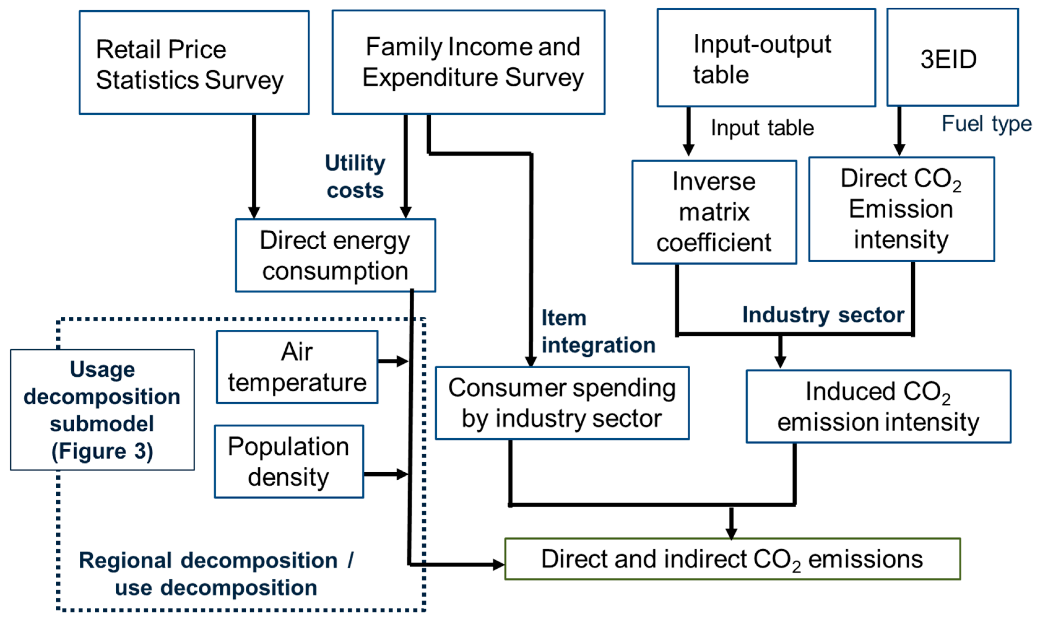
We estimated CO2 emissions using the workflow shown in Figure 2. Previous studies have estimated CO2 emissions from consumer behavior using various types of statistical data, such as input–output tables and consumption expenditure data [39,42,43]. In this study, we incorporated a usage decomposition method that considered the influence of regional conditions on direct energy consumption [41] and applied these to the consumption data for the 49 cities. This approach is based on Hirano et al. [43] and uses CO2 emissions per unit of value estimated using input–output tables and the Embodied Energy and Emission Intensity Data for Japan (3EID) [44]. We used the input–output table from the basic classification table in the basic input–output table of 2005, similar to Hirano et al. [43]. As it is difficult for wholesale and retail data in the input–output table to correspond to specific household consumption expenditures, the industrial sector margin (commercial margin) was set, and the total output was allocated based on the wholesale/retail margin of each industrial sector. As the input–output table was composed of 520 rows and 407 columns, these were aggregated into a square matrix to calculate the inverse matrix. The industrial sector classification was then set to 403, in accordance with 3EID. Based on the resulting input–output table, we calculated the inverse matrix coefficient of the [I-(IM)A]–1 type, then multiplied this by the direct CO2 emission intensity from 3EID. This provided the indirect CO2 emission intensity from household consumption expenditure. Direct CO2 emissions were calculated from the direct CO2 emission intensity based on the 3EID and domestic production values. We then calculated the indirect CO2 emission for each item of consumption expenditure using indirect CO2 emission intensity and household consumption expenditures.
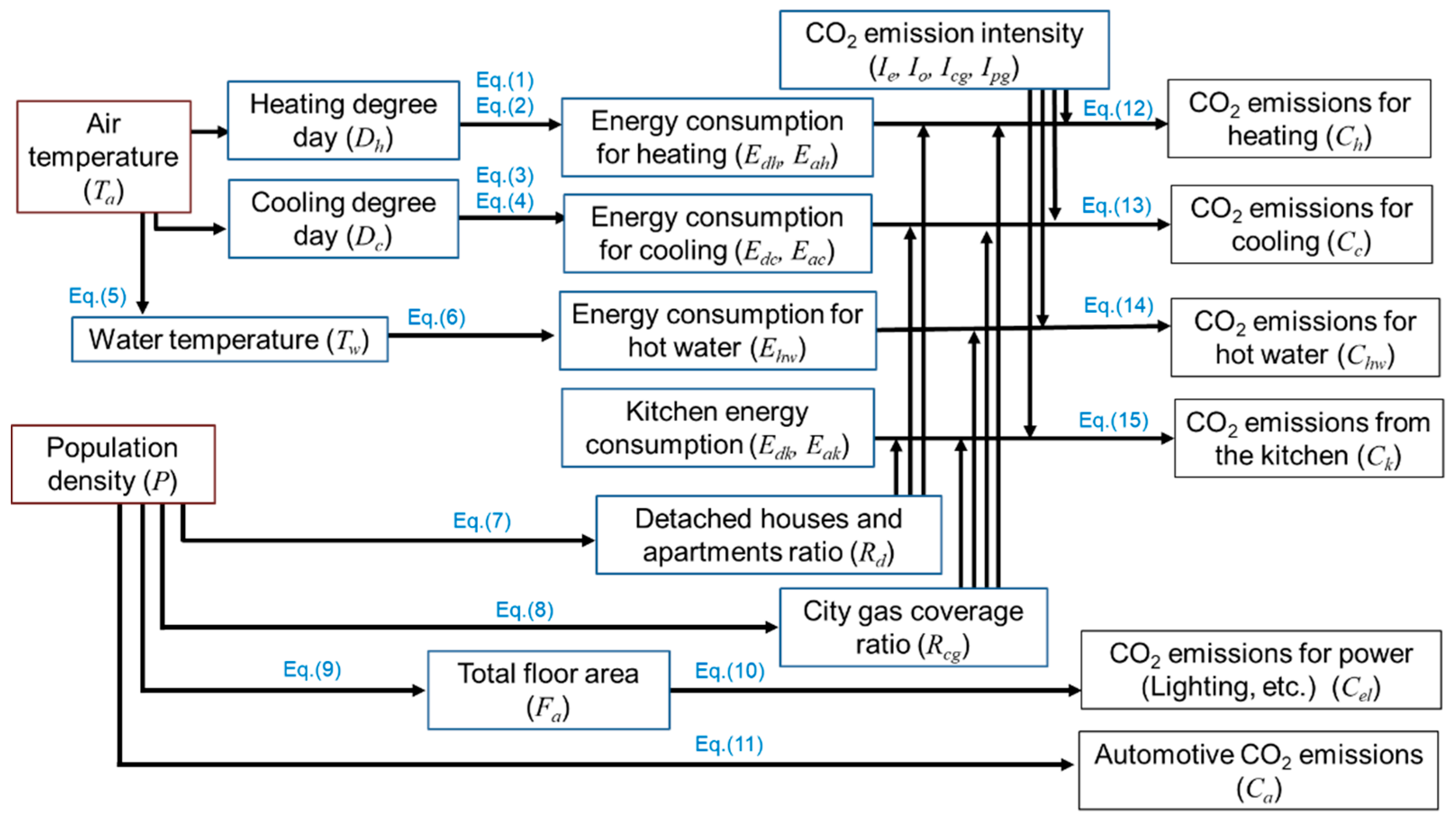
The CO2 estimation model of Hirano et al. [41] was used to develop a sub-model to estimate CO2 emissions when direct energy consumption was decomposed into energy use based on regional conditions. In this model, estimation equations created individually or known estimation equations for various factors related to CO2 emission are incorporated into the calculation. Then, by combining these estimation equations, total CO2 emissions for each energy use are estimated (Figure 3). However, for fuel, The CO2 estimation model [41] only counted in situ CO2 emissions calculated from fuel consumption and CO2 emission intensity of each fuel. For power, it only counted CO2 emissions from power plant efficiency calculated from power generation efficiency and CO2 emission intensity. On the other hand, our estimation method counted CO2 emissions related to fuel refining and transportation, and CO2 emissions associated with power consumption at power plants, as CO2 emissions due to direct energy consumption. Therefore, when incorporating these into total CO2 emissions, including indirect CO2 emissions (Section 3), we divided them into energy use by proportional allocation. The full details of this method are provided in Hirano et al. [41].
First, for space heating and cooling, energy consumption was estimated based on estimation equations by Sawachi et al. [9]. They investigated residential energy consumption in major cities across Japan with the number of valid samples of 2169 in the summer survey and 1675 in the winter survey. Based on the survey data, they analyzed the relationship between heating/cooling energy consumption and climatic conditions, and obtained the following equation by non-linear regressions (Equations (1)–(4)):
E d h = 1.25 · 10 14 · D h 5 3.49 · 10 4 · D h 2 + 2.15 · D h 155
E a h = 2.26 · 10 11 · D h 4 1.01 · 10 4 · D h 2 + 0.748 · D h + 25
E d c = 1.12 · 10 3 · D c 2 + 0.621 · D c + 18
E a c = 1.91 · 10 4 · D c 2 + 0.798 · D c + 21
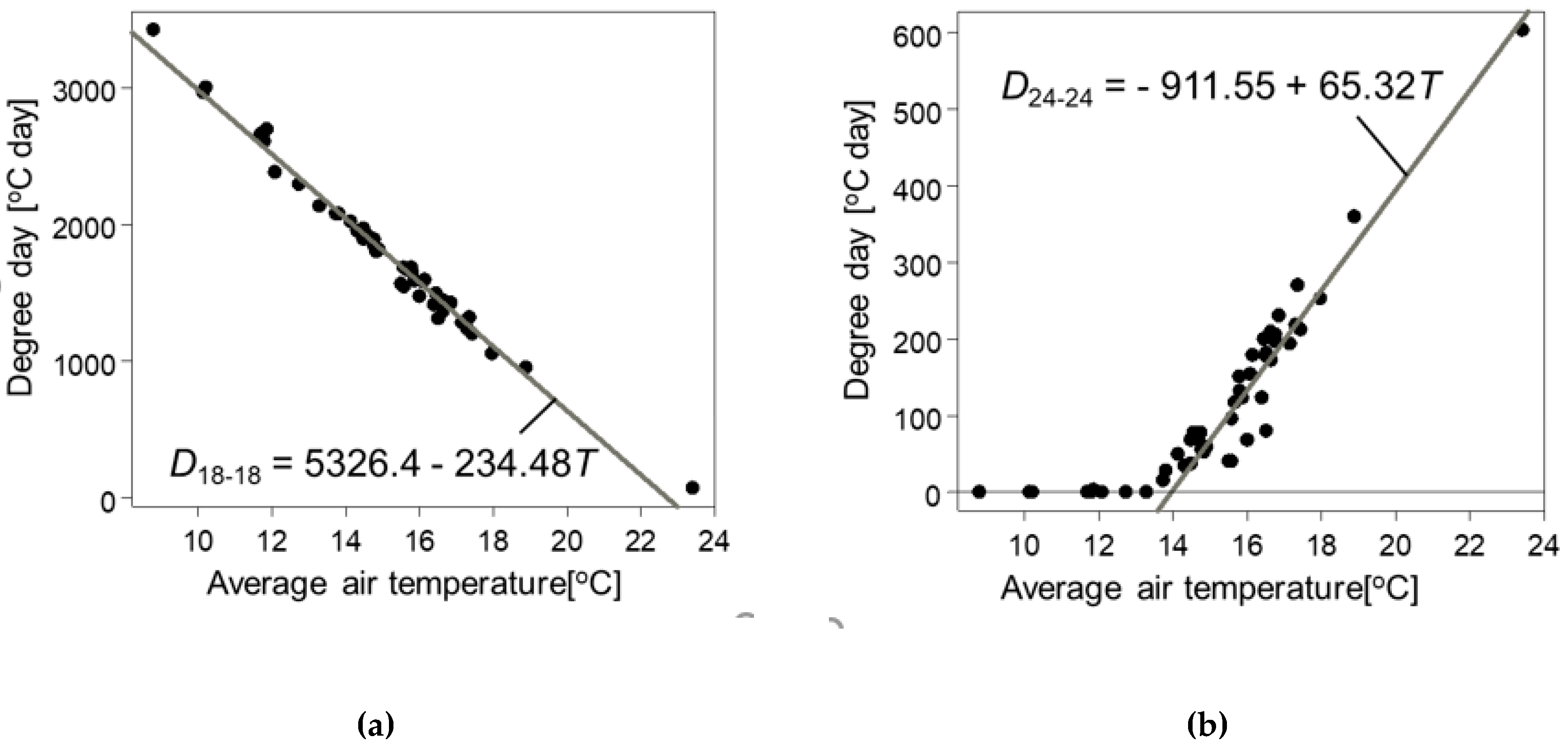
where E is secondary energy consumption (Mcal/year) (dh, detached house heating; ah, apartment heating, dc, detached house cooling; ac, apartment cooling), Dh is heating degree days (D18–18), and Dc is cooling degree days (D24–24). The heating degree days (D18–18) was defined as the cumulative total of the difference between 18 °C and the average daily temperature on days when the average daily temperature was less than 18 °C. The cooling degree days (D24–24) was defined as the sum of the difference between 24 °C and the daily average temperature on days when the daily average temperature exceeds 24 °C. In the regression analysis of Sawachi et al. [9], multiple correlation coefficients R = 0.99, 0.91, 0.94, and 0.78 were obtained in Equations (1)–(4), respectively. In Japan, although district heating and cooling are installed in some dense commercial and business areas, they are rarely installed in residential areas. As such, district heating and cooling was not considered in this model.
For hot water, the water temperature was calculated from air temperature using Equation (5) [11], and energy consumption was calculated using Equation (6) [45]:
T w = 0.7 · T a + 7.0
E h w = V · c ρ · ( T h w T w ) / η
where Ta is temperature, Ehw is energy consumption for hot water, V is the amount of hot water used, Thw is the hot water temperature, Tw is the water supply temperature, cρ is the volumetric heat capacity of water, and η is equipment efficiency. Although Equation (5) is an empirical formula, it is well known that the air temperature and the water temperature are linked, and it is a commonly used equation.
For cooking, the effect of air temperature was ignored, this was set as 4000 (MJ/household) for detached houses and 3700 (MJ/household) for apartments based on consumption per household, as presented in the existing survey data [9].
Urban density affects CO2 emissions in a variety of ways, such as the proportion of detached houses to apartments and the coverage ratio of city gas. We used population density as the parameter best representing urban density. Relationship between the ratio of houses to apartments (derived from the Population Census [46]), and the coverage ratio of city gas (derived from the purchase frequency of purchased city gas and liquid petroleum (LP) gas in the Family Income and Expenditure Survey ) and the population density of each city are shown in Figure 4 and Figure 5, respectively. These relationships were approximated by the following estimation formulas (Equations (7) and (8)):
R d = 9.09 ln ( P ) + 116
R c g = 8.77 ln ( P ) 0.804
where Rd is the detached house ratio (%), P is the population density (people/km2), and Rcg is the city gas coverage ratio (%).
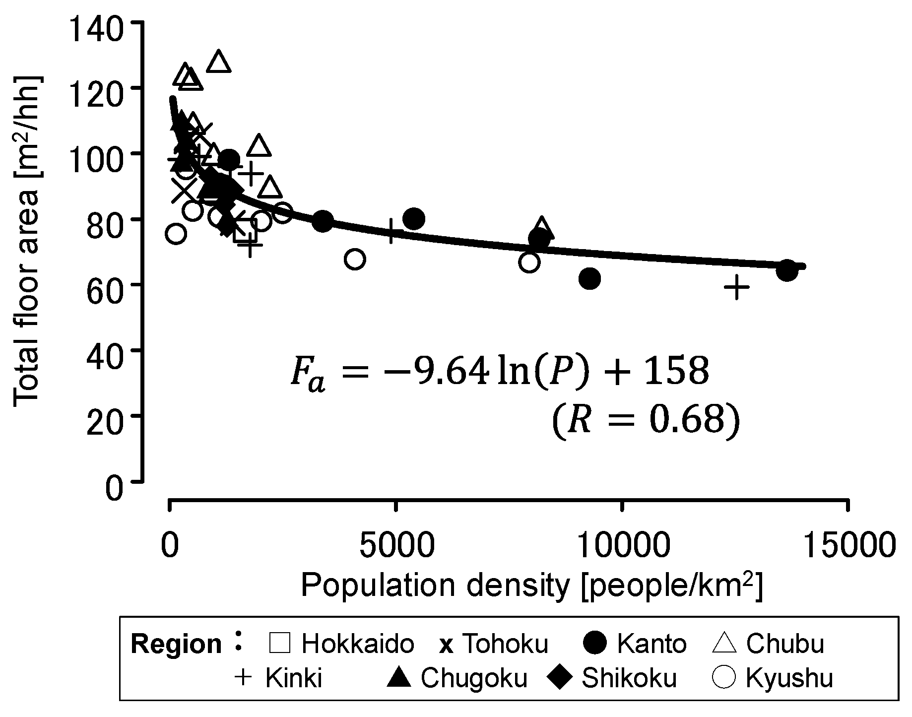
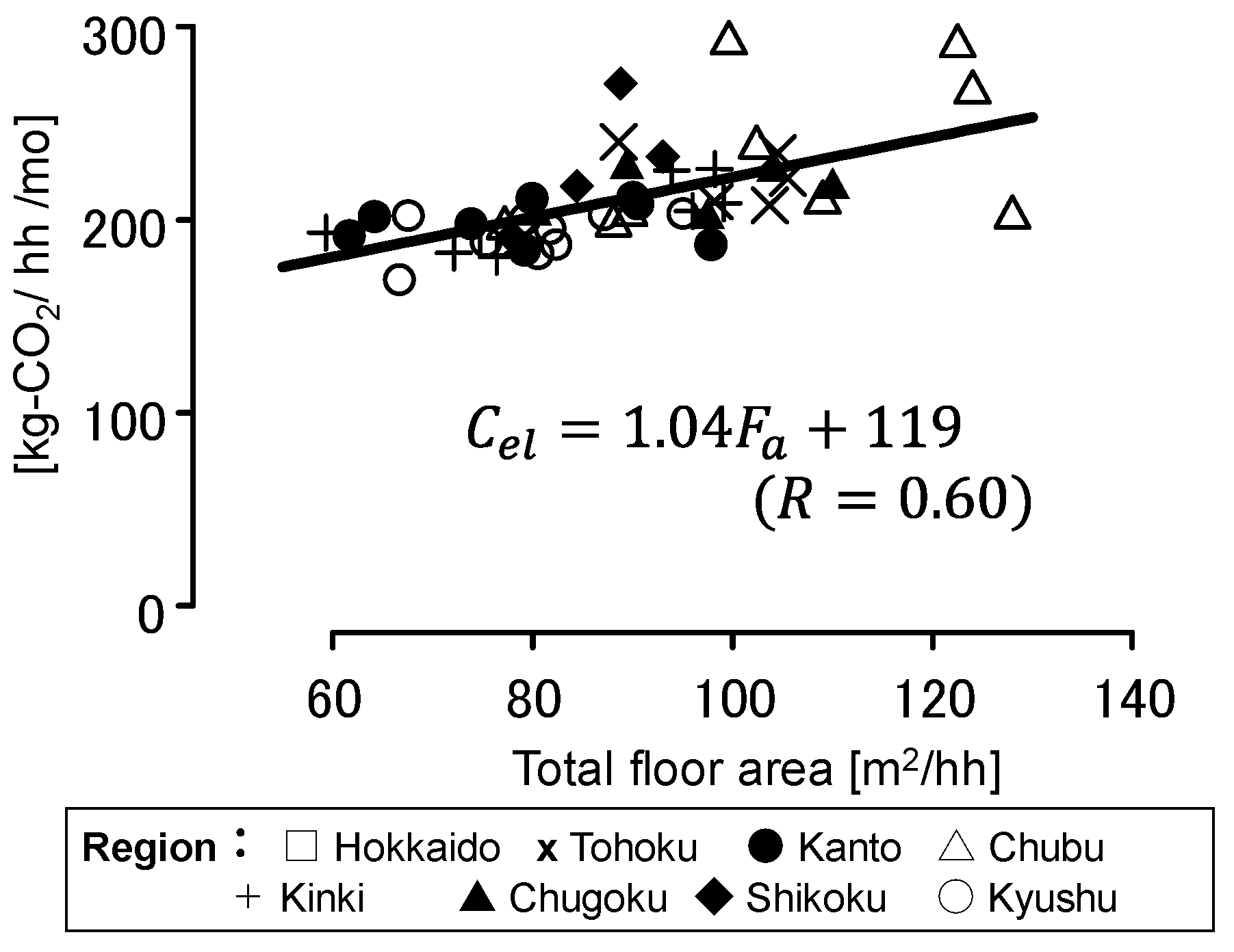
For other types of power consumption (e.g., lighting), we excluded the heating and cooling usage previously measured by calculating electricity consumption during intermediate seasons (spring and fall) using monthly values from the Family Income and Expenditure Survey and applying these values to summer and winter. As mentioned above, population density is used as an index to represent the density of cities. Although it is possible to directly relate CO2 emissions to population density empirically, it is more important to clarify the causal mechanisms for developing a general model. Therefore, we focused on the total floor area of the house, which is related to CO2 emissions. The relationship between population density and floor area and the relationship between floor area and CO2 emissions are shown in Figure 6 and Figure 7, respectively. Estimation formulas were subsequently developed for power consumption based on the population density (Equations (9) and (10)):
F a = 9.64 ln ( P ) + 158
C e l = 1.04 F a + 119
where Fa is the total floor area per household (m2/household), and Cel represents the CO2 emissions from electricity consumption during intermediate seasons (kg CO2/household/month).
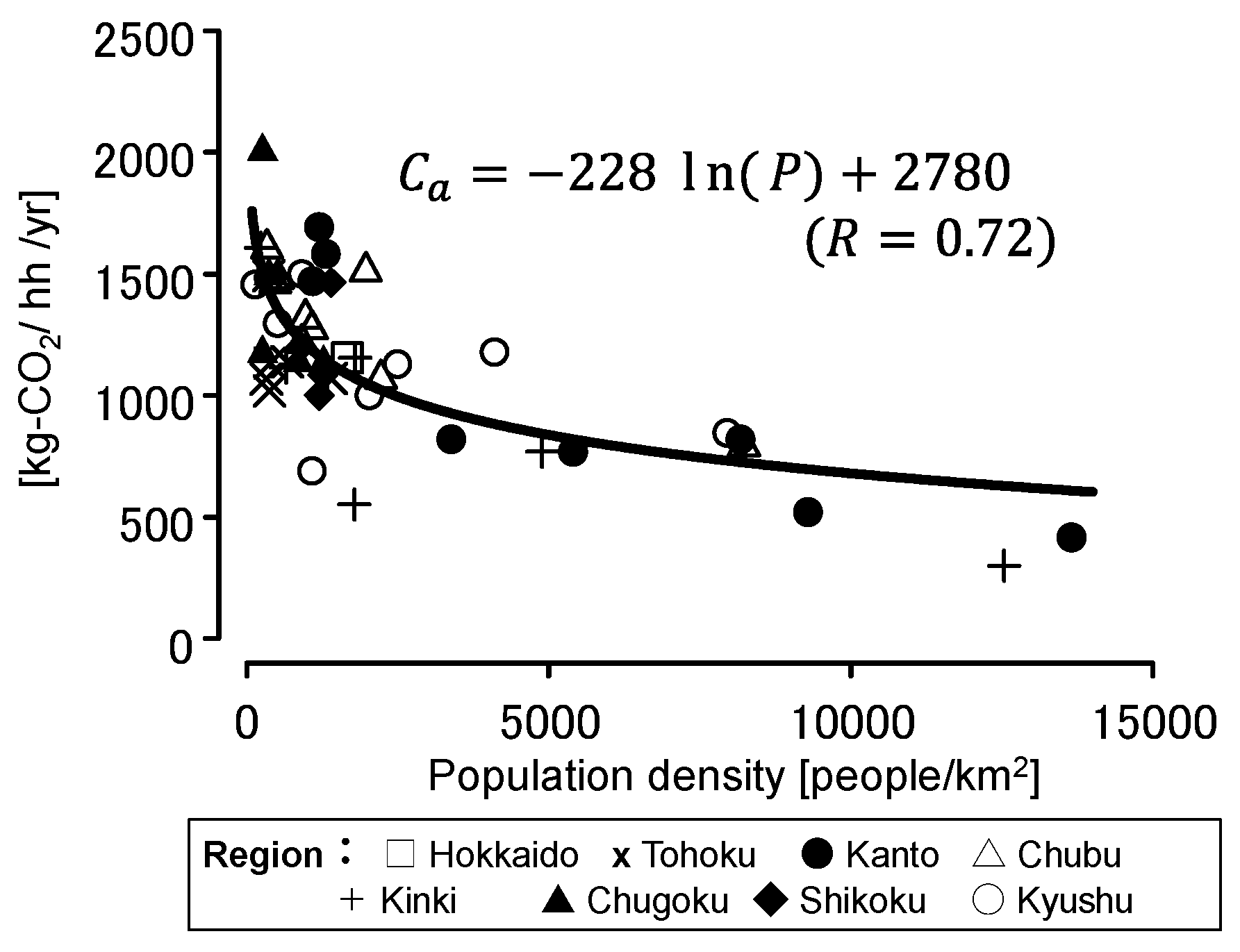
We estimated CO2 emissions from vehicle use based on the gasoline consumption calculated from the Family Income and Expenditure Survey. Relationship between the automotive CO2 emissions and the population density is shown in Figure 8. An estimation formula was then developed for gasoline consumption by cars as a function of population density (Equation (11)):
C a = 228 ln ( P ) + 2780
where Ca represents automotive CO2 emissions from gasoline consumption (kg CO2/household/year).
The source of energy used (i.e., electric or gas) was pre-determined by Hirano et al. [41] based on surveys of various existing sources (see Table 1). The CO2 emission intensity for each energy source was also set with reference to Hirano et al. [41], as shown in Table 2.
Using the above values, we calculated the CO2 emissions of heating, cooling, hot water, and kitchen by the following Equations (12)–(15).
C h = E d h · R d · ( 0.8 · I o + 0.2 · I e ) · ( 1 R c g ) + E d h · R d · ( 0.3 · I c g + 0.5 · I o + 0.2 · I e ) · R c g +   E a h · ( 1 R d ) · ( 0.8 · I o + 0.2 · I e ) · ( 1 R c g ) + E a h · ( 1 R d ) · ( 0.3 · I c g + 0.5 · I o + 0.2 · I e ) · R c g
C c = E d c · R d · I e +   E a c · ( 1 R d ) · I e
C h w = E h w · ( 0.4 · I p g + 0.6 · I o ) · ( 1 R c g ) + E h w · I c g · R c g
C k = E d k · R d · I p g · ( 1 R c g ) +   E d k · R d · I c g · R c g +   E a k · ( 1 R d ) · I p g · ( 1 R c g ) · E a k · ( 1 R d ) · I c g · R c g
where C is CO2 emissions (kg-CO2/household/year) (h, heating; c, cooling; hw, hot water; k, kitchen), E is energy consumption (MJ/ household/year) (dk, detached house kitchen; ak, apartment kitchen), I is CO2 emission intensity (kg-CO2/MJ) (e, electricity; o, kerosene; cg, city gas; pg, LP gas). It should be noted that the model of this study cannot be extrapolated to areas with a lower population density than these 49 cities.
Details of Japan’s direct energy consumption are provided in the literature [47,48,49].
Although the input–output table of 2005 was used to calculate indirect CO2 emission, since the Family Income and Expenditure Survey [40] is a sample survey, there may be variations due to sampling. Therefore, the average value from 2003 to 2007 was used to develop this model formula. We selected data over this period for analysis, recognizing that there may be a slight time lag from current emissions. This is because Japan experienced significant impacts from the 2008 financial crisis, the 2011 Great East Japan Earthquake, the resulting Fukushima Daiichi nuclear disaster, and the subsequent wide-area evacuation. Although the evacuation areas are now gradually being lifted in the current situation, considering the time lag until statistical data become available, it is difficult to obtain general results in the latest situation. We also compared several datasets on direct energy consumption in the residential sector [50] and found that inter-annual changes in the household sector were small prior to the financial crisis. Energy consumption may be decreasing due to the widespread use of light-emitting diodes (LEDs) and improved heating and cooling efficiencies of equipment. However, this change is not anticipated to be rapid as it takes time to replace buildings and equipment. In the long term, the model needs to be updated in consideration of the gradual diffusion of these new technologies.
To confirm the validity of the above equations, we compared our calculated CO2 emissions with those calculated from the Family Income and Expenditure Survey for each city, achieving a correlation coefficient of R = 0.822 (Figure 9). The model presented by Hirano et al. [41] aimed to clarify the CO2 emission structure by expressing it with essential elements rather than incorporating detailed elements in order to improve accuracy. For this reason, CO2 emissions by use were estimated based only on temperature and population density. Given the approximate nature of such parameterization, this was considered to be a relatively good match. Next, we compared the average CO2 emission values for the 49 cities by energy source, showing good correspondence (Figure 10).
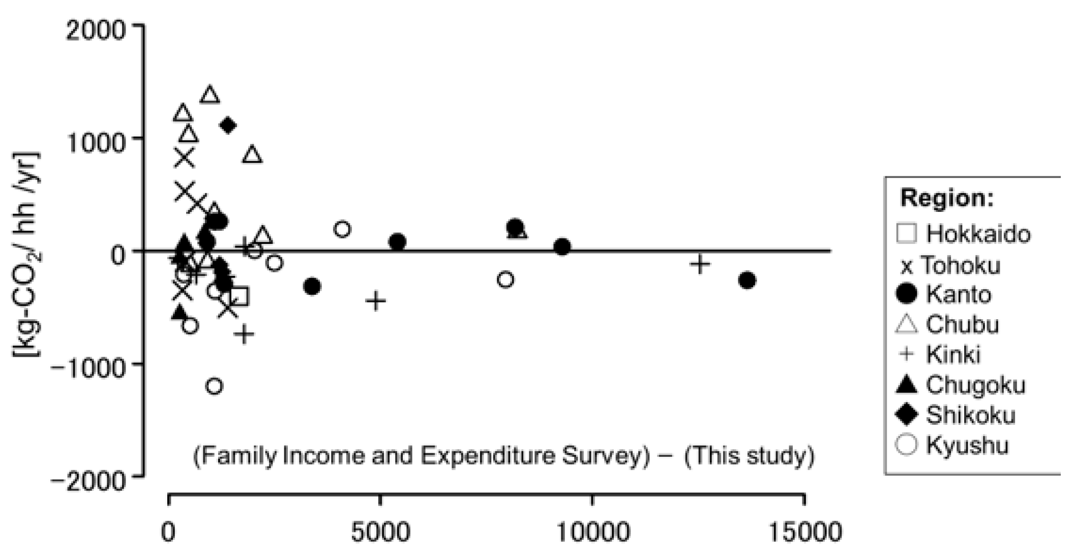
To confirm that the model is valid for all cities, we plotted the difference between the CO2 emissions calculated by the model and the CO2 emissions based on the Family Income and Expenditure Survey, and the population density (Figure 11). From this figure, it can be seen that there are relatively large variations in cities with a population density lower than 3000 (people/km2). This is because random variations due to various factors are relatively large in small cities. On the other hand, in medium and large cities with a high population density of more than 3000 (people/km2), the random variation factors are averaged and the variation is relatively small. As a whole, no clear systematic bias can be seen in Figure 11. The difference between the CO2 emissions calculated by the model and the CO2 emissions based on the Family Income and Expenditure Survey are less than -500 (kg-CO2/household/year) in 5, and more than 500 (kg-CO2/household/year) in 7 of 49 cities. Other cities are in the range of -500 (kg-CO2/household/year) to 500 (kg-CO2/household/year), and it can be said that the results are generally good when compared with the overall variation range shown in Figure 9.

3. Estimated CO2 Emissions for Each City

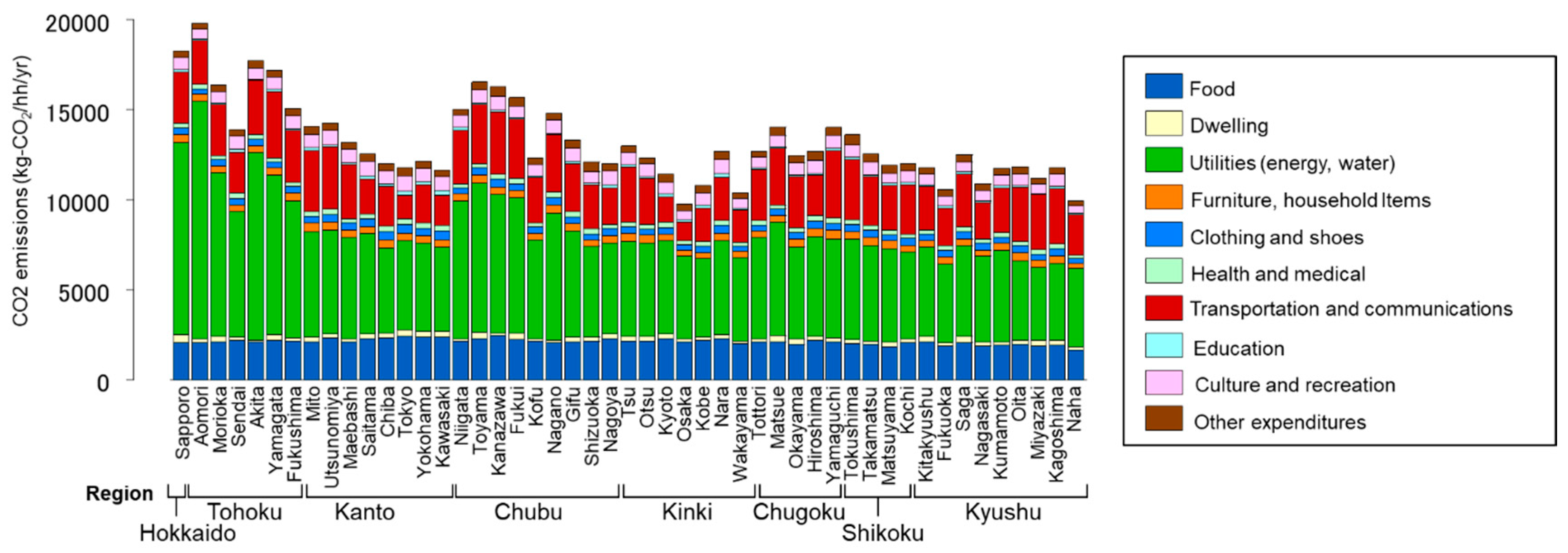
We calculated CO2 emissions by consumption behavior for each city (Figure 12). CO2 emissions were generally higher in colder regions and lower in large cities, including Tokyo and Osaka. When comparing consumption categories, the tendency for CO2 emissions to be large (especially in cold districts) was well correlated with utilities (i.e., energy and water). Thus, the influence of heating demand for interior spaces and hot water supplies was larger in the relatively colder districts. The inclination of lower CO2 emissions in large cities was for utilities (i.e., energy and water), and transportation/communication. This is likely due to a higher apartment ratio, widespread public transportation, and the shorter distances traveled. CO2 emissions from public transport were included in indirect CO2 emissions, and these were greater in large cities. However, compared to direct CO2 emissions from automobiles, indirect CO2 emissions from public transport were very small [51]. This meant that CO2 emissions were lower in large cities for the transportation and transportation categories.
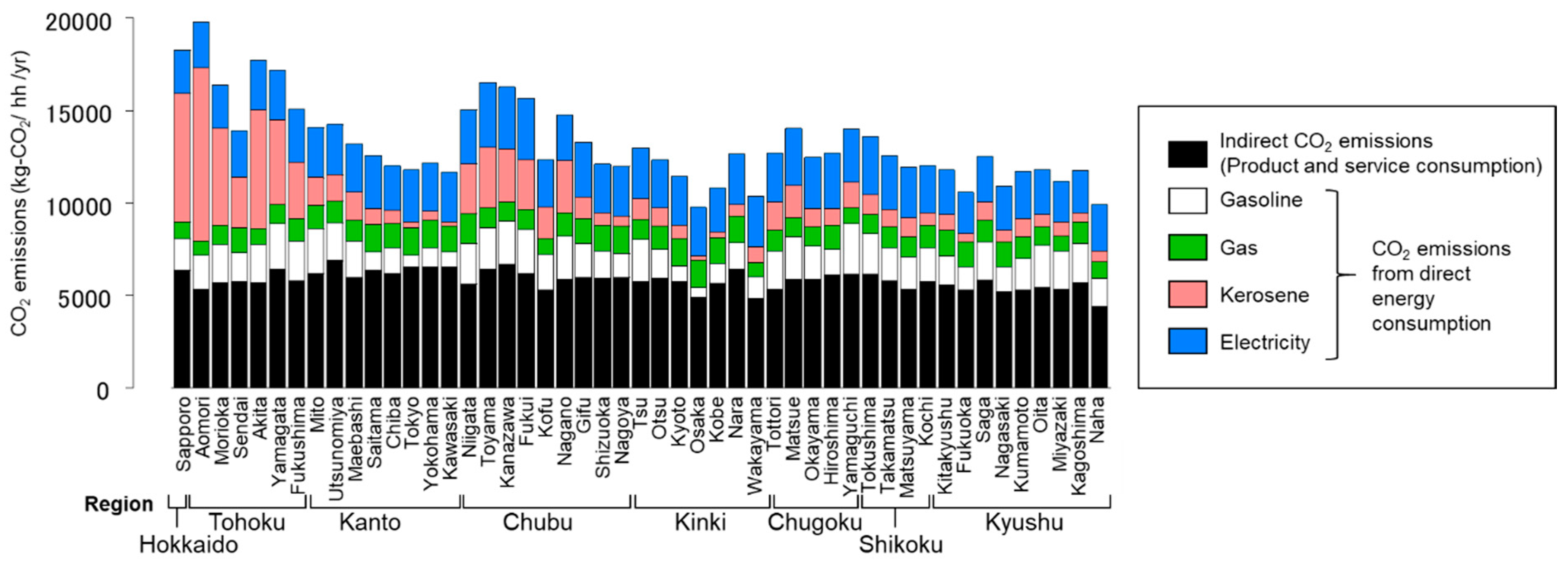
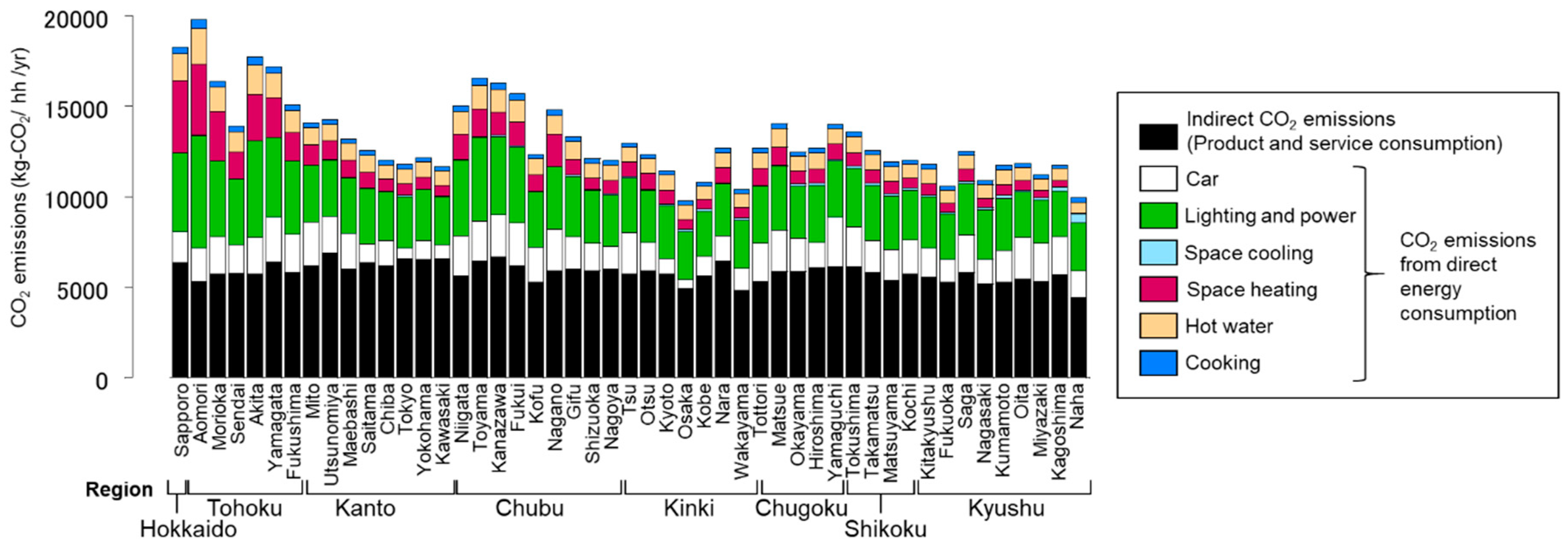
A breakdown of direct and indirect CO2 emissions by region and energy source of direct CO2 emissions (Figure 13). When CO2 emissions from electricity consumption and fuel consumption were considered as CO2 emissions due to direct energy consumption, there was some variation between cities, though on average, this was comparable to other indirect CO2 emissions. Both energy saving and indirect CO2 reductions were equally important in consumption behavior. Moreover, CO2 emissions from direct energy consumption had greater regional differences than indirect CO2 emissions. Particularly in cold regions, the level of CO2 emissions due to kerosene consumption was remarkable. This was consistent with Figure 12, as high CO2 emissions in cold regions mainly appear to be an effect of heat demand. In addition, CO2 emissions from areas, including large cities, were lower than other areas due to a reduction in car usage.
Figure 14 shows the results of decomposing CO2 emissions from energy consumption by consumers into energy use. As described above, the original calculation approach (Figure 3) used only temperature and population density and excluded CO2 emissions, such as refining and transportation, induced by energy consumption. For this reason, we adjusted the totals to the absolute amount defined in Figure 12 and Figure 13, and only the distribution ratio for each application was calculated using the workflow in Figure 3.
CO2 emissions from lighting and power accounted for approximately half of the CO2 emissions from direct energy consumption, the largest of any category. Heating demand accounted for most of the rest, while cooling and cooking were relatively minor. These findings suggest that consideration should be given to measures to improve heating supply sources, such as solar heat or cogeneration.

4. Analysis of Regional Conditions for CO2 Emissions from Direct Energy Consumption

The results so far demonstrated that the impact of regional conditions on CO2 emissions from direct energy consumption was significant. Therefore, we analyzed the effects of regional conditions in more detail using the sub-model shown in Figure 3. Although large cities tended to emit less CO2, in Japan, these cities tend to be located in relatively warm regions, making it necessary to distinguish between the effects of urbanization and those of climatic conditions when considering measures to reduce CO2 emissions.
For urban conditions, the ratio of detached houses to apartments had a relatively large effect. However, these were not presented separately in Figure 12, Figure 13 and Figure 14, preventing an assessment of their individual impact. Therefore, we selected specific major cities and calculated CO2 emissions separately for detached houses and apartments using the same values obtained from the temperature and population density in the equations above (Figure 15). The results showed a large difference between detached houses and apartments in cold regions. This may be related to the relatively low exterior roof and wall area of apartment buildings, which lowers the heating load due to reduced conduction and ventilation. On the other hand, cooling load is significantly affected by factors other than outside air, such as internal heat generation and heat obtained from window surfaces. As a result, these differences did not occur as easily in warm regions as cold regions. In addition, in the average Japanese house, energy consumption for heating is larger than energy consumption for cooling, another factor contributing to the difference between warm and cold regions.
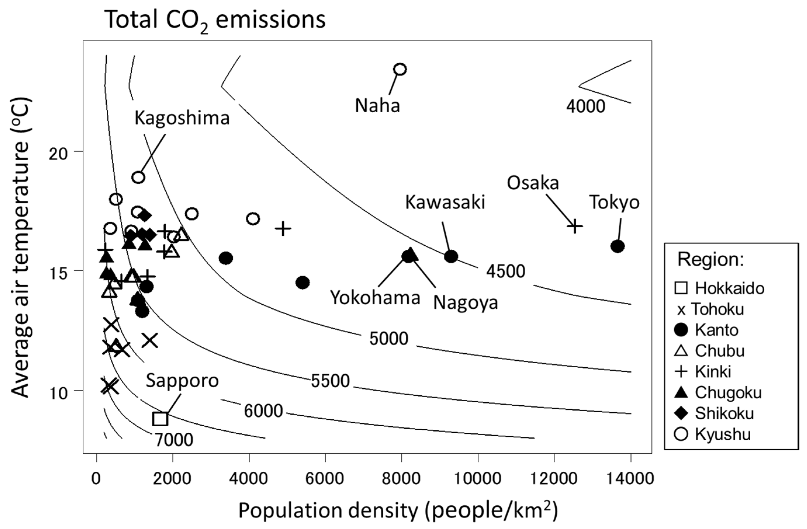
To more clearly distinguish between the effects of climatic conditions and the effects of urbanization, we considered the relationship between the two on a two-dimensional axis of population density and average temperature. First, we created estimation equations from the average temperatures and degree days in the 49 cities (Figure 16), then used these to approximate the average temperature from the degree days. This made it possible to estimate CO2 emissions in each city using only two variables, average temperature and population density (Figure 3).
We then plotted each city based on population density and average temperature, with the CO2 emissions obtained from equations in Section 2 defined by isolines (Figure 17). Overall, total CO2 emissions were lower in warmer regions because CO2 emissions in Japanese residences were more influenced by heating needs than cooling, and the influence of temperature was more likely to be higher for the former. Above an average temperature of 24 °C, the effect of cooling exceeded the effect of heating, and the isolines changed direction, though this was only applicable to 1 of the 49 cities (Naha).
We plotted similar results for heating, cooling, and hot water (Figure 18). The average temperature was the dominant factor for both heating and cooling, but population density also had a slight effect as this depends on the detached house to apartment ratio and city gas coverage ratio. For hot water, CO2 emissions were greater than for cooling, however, the effect of air temperature was smaller than for heating and cooling. These results suggest that CO2 emissions can be reduced by increasing urban density in cold regions. However, when creating new residential bases, relatively warm regions should be selected as moderate densification will likely lead to lower carbon emissions. Although there is a high possibility that CO2 emissions can be reduced by appropriately increasing density in current low-density areas, significant reductions cannot be expected even with major increases in density. This result includes suggestive findings when considering location conditions.

5. Conclusions

In this study, we calculated CO2 emissions from the consumption behavior of multi-person households in 49 Japanese cities in order to estimate both direct and indirect CO2 emissions from product and service consumption in a comparable way. The major difference between regions was CO2 emissions from direct energy consumption, which were influenced by climatic conditions and urbanization. In addition, indirect CO2 emissions from product and service consumption were almost as large as CO2 emissions from direct energy consumption, suggesting the potential to reduce CO2 emissions through lifestyle changes. The categories of utilities (i.e., energy and water) had the largest emissions, making reductions in direct CO2 emissions by energy-saving measures an important focus for future policymaking. As differences in regional conditions caused large differences in CO2 emissions from direct energy consumption, we further analyzed the effects of regional conditions on CO2 emissions per household as calculated from the sub-model used for estimating CO2 emissions from households. Regional conditions were approximated using two variables (temperature and population density), and CO2 emissions were then calculated by energy use associated with daily life. In addition, CO2 emissions tended to be higher in colder regions and lower in large cities. High CO2 emissions in cold regions were mainly caused by energy consumption for heating. This indicates that better insulation, higher efficiencies of heat source equipment, and lower heating temperature settings by adjusting clothes may be effective measures for reducing CO2 emissions. One of the most influential factors underpinning lower CO2 emissions in large cities was the low CO2 emissions from transportation. This suggests that promoting the use of public transportation and improving the fuel efficiency of automobiles may also be effective CO2 reduction measures. These results suggest the necessity for more detailed measures to reduce CO2 emissions, taking into account the substitutability of consumption behavior across the building, industrial, and transportation sectors.
Our next research topic would be the improvement of the method for data update and future prediction. At present, the efficiency of lighting, air conditioning, and automobiles is improving, and CO2 emissions may decrease with the spread of these new technologies. Therefore, the estimation equations of this study need to be updated continuously in the future. Since the method of this research is mainly based on the statistical information that is continuously surveyed in Japan, such as the Family Income and Expenditure Survey and input–output tables, it is considered possible to continuously update it in the future. Therefore, this study is meaningful as it presented the framework of the evaluation. However, in the sub-model for estimating direct energy consumption shown in Figure 3, since the heating and cooling estimation equations using degree days are based on existing research [9], it is difficult to update it using only statistical information. Therefore, we are developing a method of estimating energy consumption by heating and cooling from monthly energy consumption and temperature variation pattern. We have already proposed a method in the commercial sector to extract the variation components due to temperature from seasonal change information [52]. It is considered that our method is also applicable in the residential sector by using monthly data from the Family Income and Expenditure Survey. After continuous data acquisition becomes possible, we aim to contribute to environmental policies by forecasting and planning CO2 reductions due to the introduction of low-carbon technologies.

Author Contributions

Methodology, Y.H. and T.I.; validation, Y.H.; formal analysis, Y.H.; investigation, Y.H., T.I., M.H. and K.H.; resources, T.I. and K.H.; writing—original draft preparation, Y.H.; writing—review and editing, T.I., M.H. and K.H.; supervision, T.I. and K.H.; project administration, M.H.; funding acquisition, M.H. All authors have read and agreed to the published version of the manuscript.

Funding

This research was supported by the Environment Research and Technology Development Fund (1-1909) of the Ministry of the Environment, Japan.

Acknowledgments

We thank Tsuyoshi Fujita (National Institute for Environmental Studies), Takuya Togawa (National Institute for Environmental Studies), Daisuke Narumi (Yokohama National University) for helpful discussions and comments.

Conflicts of Interest

The authors declare no conflict of interest. The funders had no role in the design of the study; in the collection, analyses, or interpretation of data; in the writing of the manuscript, or in the decision to publish the results.

References

  1. National Institute for Environmental Studies. 2050 Low-Carbon Society Scenario. Available online: http://2050.nies.go.jp/LCS/eng/japan.html (accessed on 20 February 2020).
  2. Murakami, S.; Levine, M.D.; Yoshino, H.; Inoue, T.; Ikaga, T.; Shimoda, Y.; Miura, S.; Sera, T.; Nishio, M.; Sakamoto, Y.; et al. Overview of energy consumption and GHG mitigation technologies in the building sector of Japan. Energy Efficiency 2009, 2, 179–194. [Google Scholar] [CrossRef]
  3. Moriarty, P.; Wang, S.J. Low-carbon Cities: Lifestyle Changes are Necessary. Energy Procedia 2014, 61, 2289–2292. [Google Scholar] [CrossRef] [Green Version]
  4. Hirano, Y.; Fujita, T.; Bunya, S.; Inoue, T. Examination of how various measures in urban districts affect the development of low carbon cities-a case study of cooling energy savings in the city of Kawasaki. Environ. Sci 2011, 24, 255–268. (In Japanese) [Google Scholar]
  5. Architectural Institute of Japan. Energy Consumption for Residential Buildings in Japan; Architectural Institute of Japan: Tokyo, Japan, 2006. (In Japanese) [Google Scholar]
  6. Jyukankyo Research Institute. Residential Energy Statistics Yearbook; Jyukankyo Research Institute: Tokyo, Japan, 2011. (In Japanese) [Google Scholar]
  7. The Energy Data and Modelling Center, The Institute of Energy Economics, Japan. Handbook of Energy & Economic Statistics in Japan; The Energy Conservation Center, Japan: Tokyo, Japan, 2011. (In Japanese) [Google Scholar]
  8. Honjo, K.; Fujii, M. Impacts of demographic, meteorological, and economic changes on household CO2 emissions in the 47 prefectures of Japan. Reg. Sci. Policy Pract. 2014, 6, 13–30. [Google Scholar] [CrossRef] [Green Version]
  9. Sawachi, T.; Bohgaki, K.; Yoshino, H.; Suzuki, K.; Akabayashi, S.; Inoue, T. Energy consumption for different uses in dwelling and its estimation formulas: Study of energy consumption in residential buildings from the viewpoint of life style, on the basis of national scale surveys Part 1. J. Arch. Plann. Environ. Eng. 1994, 462, 41–48. (In Japanese) [Google Scholar]
  10. Hasegawa, Y.; Inoue, T. Energy consumption in housing on the basis of national scale questionnaire: Study on influence of residential characteristic and dispersion of energy consumption part1. J. Envrion. Eng. 2004, 583, 23–28. (In Japanese) [Google Scholar] [CrossRef]
  11. Ishida, K. Energy consumption of detached houses. J. Arch. Plann. Envrion. Eng. 1997, 501, 29–36. (In Japanese) [Google Scholar]
  12. Nansai, K.; Kagawa, S.; Kondo, Y.; Suh, S.; Inaba, R.; Nakajima, K. Improving the completeness of product carbon footprints using a global link input-output model: The case of Japan. Econ. Syst. Res. 2009, 21, 267–290. [Google Scholar] [CrossRef]
  13. Nansai, K.; Moriguchi, Y. Practical determination of sectoral environmental burdens applied to input-output analysis. J. Life Cycle Assess. Jpn. 2006, 2, 22–41. (In Japanese) [Google Scholar] [CrossRef]
  14. Koide, R.; Lettenmeier, M.; Kojima, S.; Toivio, V.; Amellina, A.; Akenji, L. Carbon Footprints and Consumer Lifestyles: An Analysis of Lifestyle Factors and Gap Analysis by Consumer Segment in Japan. Sustainability 2019, 11, 5983. [Google Scholar] [CrossRef] [Green Version]
  15. Diamond, R. A lifestyle-based scenario for US buildings: Implications for energy use. Energy Policy 2003, 31, 1205–1211. [Google Scholar] [CrossRef] [Green Version]
  16. Shimoda, Y.; Fujii, T.; Morikawa, T.; Mizuno, M. Residential End-Use Energy Simulation at City Scale. Build. Envrion. 2004, 39, 959–967. [Google Scholar] [CrossRef]
  17. Genjo, K.; Tanabe, S.; Matsumoto, S.; Hasegawa, K.; Yoshino, H. Relationship between possession of electric appliances and electricity for lighting and others in Japanese households. Energy Build. 2005, 37, 259–272. [Google Scholar] [CrossRef]
  18. Lopes, L.; Hokoi, S.; Miura, H.; Shuhei, K. Energy efficiency and energy savings in Japanese residential buildings-research methodology and surveyed results. Energy Build. 2005, 37, 698–706. [Google Scholar] [CrossRef]
  19. Shimoda, Y.; Asahi, T.; Taniguchi, A.; Mizuno, M. Evaluation of City-Scale Impact of Residential Energy Conservation Measures Using the Detailed End-Use Simulation Model. Energy 2007, 32, 1617–1633. [Google Scholar] [CrossRef]
  20. Bartiaux, F. Does environmental information overcome practice compartmentalisation and change consumers’ behaviours? J. Clean. Prod. 2008, 16, 1170–1180. [Google Scholar] [CrossRef]
  21. Gyberg, P.; Palm, J. Influencing households’ energy behaviour-how is this done and on what premises? Energ Policy 2009, 37, 2807–2813. [Google Scholar] [CrossRef]
  22. Ouyang, J.; Hokao, K. Energy-saving potential by improving occupants’ behavior in urban residential sector in Hangzhou City, China. Energy Build. 2009, 41, 711–720. [Google Scholar] [CrossRef]
  23. Almeida, A.D.; Fonseca, P.; Schlomann, B.; Feilberg, N. Characterization of the household electricity consumption in the EU, potential energy savings and specific policy recommendations. Energy Build. 2011, 43, 1884–1894. [Google Scholar] [CrossRef]
  24. Gouveia, J.P.; Fortes, P.; Seixas, J. Projections of energy services demand for residential buildings: Insights from a bottom-up methodology. Energy 2012, 47, 430–442. [Google Scholar] [CrossRef]
  25. Sanquist, T.F.; Orr, H.; Shui, B.; Bittner, A.C. Lifestyle factors in U.S. residential electricity consumption. Energy Policy 2012, 42, 354–364. [Google Scholar] [CrossRef]
  26. Meester, T.D.; Marique, A.F.; Herde, A.D.; Reiter, S. Impacts of occupant behaviours on residential heating consumption for detached houses in a temperate climate in the northern part of Europe. Energy Build. 2013, 57, 313–323. [Google Scholar] [CrossRef]
  27. Hu, T.; Yoshino, H.; Jiang, Z. Analysis on urban residential energy consumption of Hot Summer & Cold Winter Zone in China. Sustain. Cities Soc. 2013, 6, 85–91. [Google Scholar]
  28. Pisello, A.L.; Piselli, C.; Cotana, F. Influence of human behavior on cool roof effect for summer cooling. Build. Environ. 2015, 88, 116–128. [Google Scholar] [CrossRef]
  29. Shiraki, H.; Nakamura, S.; Ashina, S.; Honjo, K. Estimating the hourly electricity profile of Japanese households-coupling of engineering and statistical methods. Energy 2016, 114, 478–491. [Google Scholar] [CrossRef] [Green Version]
  30. Lubashevskiy, V.; Hirano, Y. Prediction of Power Supply Demand: Consumption Pattern Modeling. Int. J. Adv. Sci. Eng. Technol. 2018, 6, 61–66. [Google Scholar]
  31. Fun to Share Campaign. Available online: http://funtoshare.env.go.jp/ (accessed on 20 February 2020). (In Japanese)
  32. Eco-Home Diagnosis (Uchi-Eco Shindan). Available online: http://www.uchi-eco.com/index.php (accessed on 20 February 2020).
  33. National Institute for Environmental Studies. Greenhouse Gas Inventory Office of Japan, Greenhouse Gas Inventory. Available online: http://www-gio.nies.go.jp/index.html (accessed on 20 February 2020).
  34. Bin, S.; Dowlatabadi, H. Consumer lifestyle approach to US energy use and the related CO2 emission. Energy Policy 2005, 33, 197–208. [Google Scholar] [CrossRef]
  35. Liu, L.; Wu, G.; Wang, J.; Wei, Y. China’s carbon emissions from urban and rural households during 1992-2007. J. Clean. Prod. 2011, 19, 1754–1762. [Google Scholar] [CrossRef]
  36. Dai, H.; Masui, T.; Matsuoka, Y.; Fujimori, S. The impacts of China’s household consumption expenditure patterns on energy demand and carbon emissions towards 2050. Energy Policy 2012, 50, 736–750. [Google Scholar] [CrossRef]
  37. Wang, Z.; Yang, L. Indirect carbon emissions in household consumption: Evidence from the urban and rural area in China. J. Clean. Prod. 2014, 78, 94–103. [Google Scholar] [CrossRef]
  38. Weber, C.; Perrels, A. Modelling lifestyle effects on energy demand and related emissions. Energy Policy 2000, 28, 549–566. [Google Scholar] [CrossRef]
  39. Hirano, Y.; Ihara, T.; Yoshida, Y. Estimating Residential CO2 Emissions based on Daily Activities and Consideration of Methods to Reduce Emissions. Build. Environ. 2016, 103, 1–8. [Google Scholar] [CrossRef]
  40. Statistics Bureau of Japan, Ministry of Internal Affairs and Communications. Family Income and Expenditure Survey. Available online: http://www.stat.go.jp/data/kakei/ (accessed on 21 February 2020). (In Japanese)
  41. Hirano, Y.; Fujita, T.; Takahashi, T. Examination and formulation of household CO2 emissions and energy uses in major cities in Japan. Environ. Syst. Res. 2010, 38, 309–316. (In Japanese) [Google Scholar]
  42. Ihara, T.; Motose, R.; Kudoh, Y. Consideration of Analysis on CO2 Emissions from Household Expenditure with Input-Output Tables. Proc. Ann. Meet. Environ. Syst. Res. 2009, 37, 267–273. (In Japanese) [Google Scholar]
  43. Hirano, Y.; Ihara, T.; Togawa, T.; Gomi, K.; Okuoka, K.; Kobayashi, G. Investigation of Low-carbon Lifestyles Based on Direct/Indirect Residential CO2 Emissions. Environ. Sci 2017, 30, 261–273. (In Japanese) [Google Scholar]
  44. National Institute for Environmental Studies. 3EID-Embodied Energy and Emission Intensity Data for Japan Using Input-Output Tables. Available online: http://www.cger.nies.go.jp/publications/report/d031/eng/index_e.htm (accessed on 21 February 2020).
  45. LP-GAS Annual Report Fact Figures; Sekiyu-Kagaku-Shimbun-Sha: Tokyo, Japan, 2005.
  46. Statistics Bureau of Japan, Ministry of Internal Affairs and Communications. Population Census. Available online: https://www.stat.go.jp/english/data/kokusei/index.html (accessed on 21 February 2020).
  47. Murakami, S.; Levine, M.D.; Yoshino, H.; Inoue, T.; Ikaga, T.; Shimoda, Y.; Miura, S.; Sera, T.; Nishio, M.; Sakamoto, Y.; et al. Energy Consumption, Efficiency, Conservation, and Greenhouse Gas Mitigation in Japan’s Building Sector; Lawrence Berkeley National Laboratory, Institute for Building Environment and Energy Conservation: Berkeley, CA, USA, 2006. [Google Scholar]
  48. The Institute of Energy Economics. EDMC Handbook of Japan’s & World Energy & Economic Statistics; The Energy Conservation Center: Tokyo, Japan, 2017. [Google Scholar]
  49. Agency for Natural Resources and Energy. Japan’s Energy 2019–10 Questions for Understanding the Current Energy Situation. Available online: https://www.enecho.meti.go.jp/en/category/brochures/pdf/japan_energy_2019.pdf (accessed on 21 February 2020).
  50. Hirano, Y.; Fujita, T. Evaluation of the impact of the urban heat island on residential and commercial energy consumption in Tokyo. Energy 2012, 37, 371–383. [Google Scholar] [CrossRef]
  51. Hirano, Y.; Gomi, K.; Togawa, T.; Ariga, T.; Matsuhashi, K.; Fujita, T. The Relationship Between CO2 Emissions from Urban Traffic and Urban Area Density. J. Jpn. Soc. Civ. Eng. Ser. G (Environ. Res.) 2018, 74, II_183–II_191. (In Japanese) [Google Scholar]
  52. Hirano, Y.; Gomi, K.; Nakamura, S.; Yoshida, Y.; Narumi, D.; Fujita, T. Analysis of the impact of regional temperature pattern on the energy consumption in the commercial sector in Japan. Energy Build. 2017, 149, 160–170. [Google Scholar] [CrossRef]
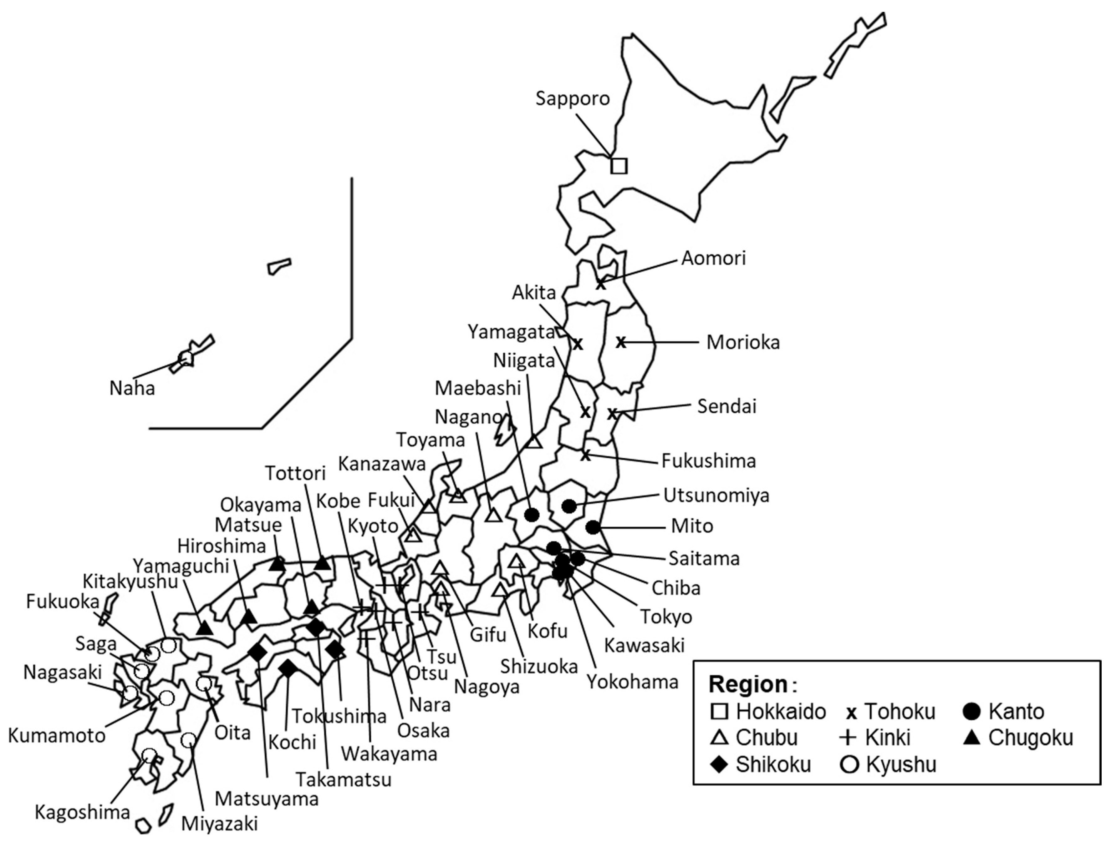
Figure 1. Distribution of the 49 Japanese cities considered in this study.
Sustainability 12 04678 g001
Figure 2. CO2 emission estimation workflow used in this study.
Sustainability 12 04678 g002
Figure 3. Calculation workflow of the direct CO2 emissions estimation sub-model.
Sustainability 12 04678 g003
Figure 4. Relationship between the detached house ratio and the population density (modified from Hirano et al. [41]).
Sustainability 12 04678 g004
Figure 5. Relationship between the city gas coverage ratio and the population density (modified from Hirano et al. [41]).
Sustainability 12 04678 g005
Figure 6. Relationship between the total floor area per household and the population density (modified from Hirano et al. [41]).
Sustainability 12 04678 g006
Figure 7. Relationship between the CO2 emissions during intermediate seasons and the total floor area (modified from Hirano et al. [41]).
Sustainability 12 04678 g007
Figure 8. Relationship between the automotive CO2 emissions and the population density (modified from Hirano et al. [41]).
Sustainability 12 04678 g008
Figure 9. Correlation between CO2 emissions calculated by this study and the Family Income and Expenditure Survey for 49 cities.
Sustainability 12 04678 g009
Figure 10. Comparison of CO2 emissions calculated by this study and the Family Income and Expenditure Survey with the estimated value by energy source.
Sustainability 12 04678 g010
Figure 11. A plot of the difference between CO2 emissions calculated by this study and the Family Income and Expenditure Survey versus the population density.
Sustainability 12 04678 g011
Figure 12. CO2 emissions by consumption behavior for multi-person households.
Sustainability 12 04678 g012
Figure 13. CO2 emissions by energy source for multi-person households.
Sustainability 12 04678 g013
Figure 14. CO2 emissions by energy use for multi-person households.
Sustainability 12 04678 g014
Figure 15. Estimated CO2 emissions for detached houses and apartments.
Sustainability 12 04678 g015
Figure 16. Relationship between average temperature and degree days for the 49 Japanese cities. (a) Heating degree days (D18-18); (b) Cooling degree days (D24-24).
Sustainability 12 04678 g016
Figure 17. Isolines for total CO2 emissions calculated from population density and average temperature based on the workflow shown in Figure 3.
Sustainability 12 04678 g017
Figure 18. Isolines for CO2 emissions related to residential heating, cooling, and hot water calculated from population density and average temperature based on the workflow shown in Figure 3.
Sustainability 12 04678 g018
Table 1. Setting values of energy source configuration [41].
Energy ApplicationsHouseholds Using City GasHouseholds Using LP Gas
Space heatingCity gas: 30%
Kerosene: 50%
Electricity: 20%
Kerosene: 80%
Electricity: 20%
Space coolingElectricity: 100%Electricity: 100%
Hot waterCity gas: 100%LP gas: 40%
Kerosene: 60%
CookingCity gas: 100%LP gas: 100%
Table 2. Setting values of CO2 emission intensity.
Energy SourceCO2 Emission Intensity (kg-CO2/MJ)
Electricity (secondary energy)0.1541
Kerosene0.0678
City Gas0.0511
LP gas0.0600