1. Introduction
1.1. Background and Research Objectives
Freight rail transportation relies on a fleet of circulating rail cars, either within specific service routes or areas or across the whole rail network. In addition to track infrastructure [
1], operational restrictions [
2] and service schedules [
3], the capacity of rail transportation is directly related to the number of available rail cars and how efficiently they are circulated [
4]. Rail cars are investments for their operators/owners and the return of investment depends mainly on their usage. From the perspective of rail car owners and railway operators, the objective is to always keep the cars moving, as they only provide revenue (excluding demurrage) when carrying a load. Therefore, any idling of a car is undesired. On the other hand, from the shippers’ perspective, the objective is to have a rail car available when it is needed to avoid any unplanned loss of productivity and related storage costs.
Determining the optimal number of rail cars that meets the expectations of both shippers and operators/owners is a challenging task, further complicated by potential seasonal fluctuations in freight volumes. The challenge gets even more complicated if the number of origins, destinations and possible routes is large. The forest products movements (especially transportation of logs to the mills) in the Upper Midwest region (the Upper Peninsula of Michigan, Wisconsin and Minnesota) of the US is one example of a challenging location for sizing a rail car fleet. Moving logs by rail from aggregation points to the mills has been a very cost effective and safe method of moving raw materials. Using rail has also provided social benefits by reducing the number of heavy log trucks on public highways and related emissions from the trucks [
5]. However, recent rail rate increases are pushing more logs into truck transportation. One of the justifications for increased rail rates has been a need for the replacement of the rail car fleet, as many rail cars are close to reaching the end of their service life. However, neither shippers nor railroads have a clear understanding of the proper size of such a fleet that would meet the demands in the region and maintain the rail as a sustainable alternative for the industry.
One fleet replacement alternative is the formation of a dedicated fleet of rail cars shared by all industry companies in the region. Shared fleet is expected to improve the efficiency of how cars are used, as cars no longer are limited to the origin–destination (OD) pairs of any individual company but can rather function as a single region-wide pool. This way, each car can be sent to the nearest location where it is needed, regardless of the specific company making the request. To secure funding for such a fleet, there is a need to determine the proper size of the fleet based on the efficient utilization of the cars.
This rail car fleet size study on freight storage and car idling was conducted to provide the industry with insights and benchmarking values for the openly accessible fleet size in ideal conditions. It explores the number of rail cars in the region, considering an actual database collected from the forestry companies. It also provides scenarios to evaluate how the number of cars affects the storage need at the sidings and the time the cars are idled. The analysis is the first step toward justifying investment in cars that is needed to continue and hopefully expand the log movements on rails and the overall sustainability of rail networks in the region.
1.2. Literature Review
Several studies have addressed the challenges of sizing the rail car fleet [
6,
7,
8,
9,
10,
11], with most studies focusing on a particular methodology to define the optimized fleet size. For example, Sherali and Maguire [
6] suggested the coordinated use of static and dynamic fleet-sizing models to determine the minimum fleet size for providing adequate service to an automobile company. Bojovic [
7] developed a mathematical model based on the general system theory to determine an optimal number of rail freight cars that satisfy a demand for the transportation of goods on a railroad network under consideration. Sayarshad and Ghoseiri [
8] proposed a heuristic method to optimize the fleet size and freight car allocation, assuming car demand and travel times are deterministic and unmet demands are backordered. Yaghini and Khandaghabadi [
9] further developed the model by adding rail car ownership, holding empty cars at stations, and adding departure and arrive schedule for cars. Milenkovic and Bojovic [
10] developed a fuzzy linear dynamic model of rail car flows in a network considering uncertain demands.
Rail car fleet sizing models are also highly related to the studies that consider distribution problem of empty rail cars [
12,
13,
14,
15]. White and Bomberault [
12] provided one of the earliest studies of the empty car distribution problem using a network-flow model. Joborn et al. [
13] proposed a capacitated network-design model that considers economies of scale for the distribution of empty cars, and developed a tabu search heuristic algorithm that can be applied at both the tactical and strategic levels. Narisetty et al. [
14] developed the mathematical model to create a tool to provide quantitative answers to questions about the car-assignment problem. The model seeks to reduce transportation costs and improve delivery time and customer satisfaction. More recently, Heydari and Melachrinoudis [
15] developed the empty railcar distribution model considering the block and capacity of trains.
One of the limitations of the studies reviewed above is their reliance on virtual networks and freight flows to test the models. For example, Bojovic [
7] tested his model on a hypothetical network with five stations, and Milenkovic and Bojovic [
10] also demonstrated the numerical example on the network with two stations on a four-day planning horizon. Another limitation of previous studies seems to be the absence of detailed data on actual rail operations (e.g., the rail transit time estimation from real routes/schedule of trains). If such data was available or used, it was not reported in studies reviewed. For detailed models, the knowledge of the rail transit time between all origin–destination pairs is one of the critical factors when identifying the number of rail cars needed. Previous studies have estimated rail transit time by either the probability distribution function, such as the fuzzy Gaussian probability density function [
10], or by using historical data for the same OD pairs [
16]. We have approached the challenge by developing the rail transit time function based on real train schedule and routing data obtained from the rail service provider.
Overall, our study expands the body of knowledge in the rail car fleet sizing problem by: (1) providing an improved understanding of the impact of rail car fleet size and loading/unloading efficiency on freight storage and car idling, and (2) actual and detailed industry shipment and rail operation data as the foundation for methodology and analysis, as provided by the involved shippers and rail carriers.
2. Materials and Methods
2.1. Log Movement Data Collection
Our research relied on a confidential and comprehensive dataset of log movements to 11 mills in the region during the calendar year of 2017, provided by five forest industry companies of the Lake State Shippers Association (LSSA). The main study area covers the state of Wisconsin, Minnesota, and the Upper Peninsula (UP) of Michigan in the US. The data from each mill included the following: the origin and destination of log shipments (from forest landing, or rail siding to the mill), the quantity transported (tons or cords), the transportation costs, the date, a unique identifier (trip ticket number), and the rail sidings utilized (as necessary). While the identifiable data on individual shipments and mills cannot be released due to confidentiality, the LSSA website [
17] provides more information on the research project and the source of the data.
Table 1 provides summary of the log movement data used in the project. The confidential data were collected by mail with a secured flash drive or by upload to a secured cloud storage. As shown in
Table 1, we used 15,740 log tickets (we assumed one ticket indicated one rail car) for a total of 1,342,603 tons of log movements by rail for the analysis. Although we knew the modal distribution between rail cars and trucks, our sample concentrated on logs currently moving by rail cars. Hence, the logs moving to mills by trucks were excluded from this specific analysis. For infrastructure data, we used the actual rail network and rail sidings status data provided by US Department of Transportation (DOT) [
18] and by the regional rail carriers.
Table 2 provides the monthly averages for the log tickets moved by rail. There are great differences between the mills, as some of the mills rely mainly on truck movements. There are also fluctuations between the months, mainly due to seasonal harvesting or transportation conditions. April has the lowest number of tickets (1042) and September the highest (1576).
2.2. Rail Operations Data Collection
In addition to the log shipments, data from rail operations in the study area was collected directly from the main rail carriers operating in our study area. CN Railway (CN) and Escanaba & Lake Superior Railroad (E&LS) are the main Class 1 and regional rail carrier in this region, respectively. As detailed rail operation data is not publicly available, many past studies have not accounted for specific train schedules and operations, but rather assumed rail as “shortest path” movements and trains stopping at each siding to pick-up and/or drop-off cars. CN graciously shared detailed data and schedules for 35 trains operating between 72 OD pairs in the region with the research team, which was critical for the detailed operational analysis. For E&LS, the operational snapshot from the operations and train delay reports (TDRs) during the last quarter of 2018 was provided. Since the rail operation data, such as train routings and schedules, are confidential, the specific values are not included in the paper. The data used in the analysis included each train origin–destination, functions at each siding (drop/pick-up/pass), schedules at each location, days of operation and connecting trains at yards. The availability of this data allowed us to build realistic route plans that meet the trains’ actual paths and schedules.
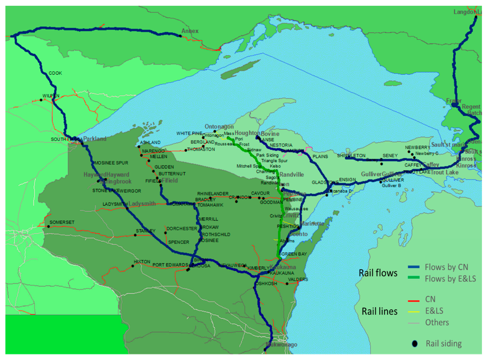
The GIS map in
Figure 1 depicts all current rail tracks and the rail sidings in study area, although some of the segments and sidings have been out of service for extended period of time.
Figure 1 also shows the main rail routes of log movement, created based on the rail shipment data collected for this project. All geographical preprocessing and spatial analysis were conducted using ESRI ArcMap 10.3.
2.3. Rail Transit Time Estimation Model
The analysis investigated the rail car fleet size needed for moving logs in the study area and the impact of the fleet size and loading/unloading time on rail car idling and on intermediate log storage needs prior to rail transportation. We developed a large-scale Integer Linear Programming (ILP) model to estimate the number of rail cars needed in the study area. We applied the model to two scenarios:
Scenario 1: Logs move by rail as soon as they arrive (eliminate storage).
Scenario 2: Logs can be moved immediately or temporarily stored at the siding as they arrive (storage available as alternative).
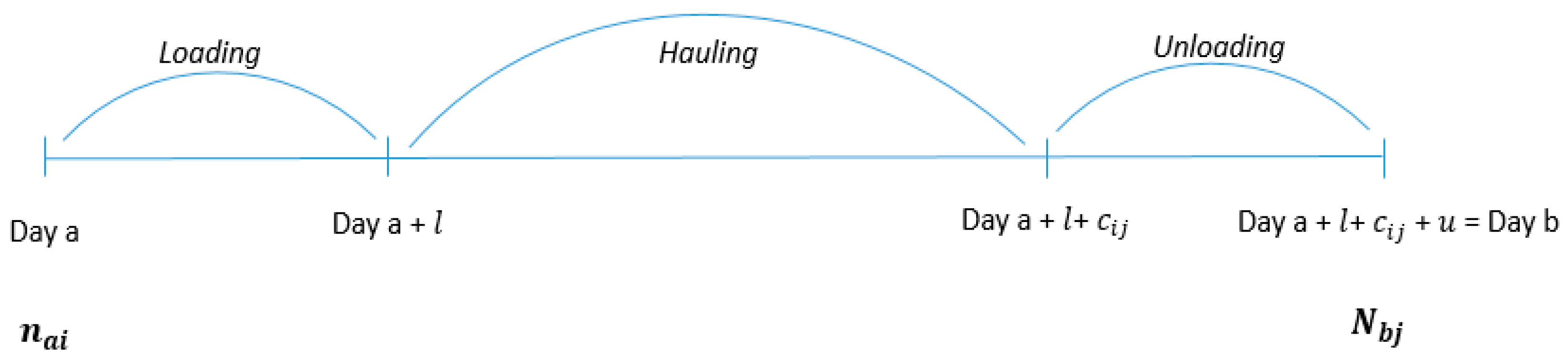
For both scenarios, we assumed that the total time to ship the logs consisted of the loading time at the origin site, the hauling time, and the unloading time at the destination (
Figure 2).
In
Figure 2,
indicates the rail hauling days to move from origin
i to mill
j (same as
j to
i); the loading/unloading days are expressed by
l and
u, respectively;
means the number of rail cars about to be loaded at the origin
i at day
a; and
indicates the number of rail cars that finish unloading at the mill
j at day
b. An empty rail car at day
b can be reassigned to any other rail siding for loading.
Since we already knew the day
b based on the log movement data collected from the forest companies, it would be possible to calculate day
a if we knew the rail hauling days. However, such estimation of rail hauling days (
in
Figure 2) is challenging as there is little information on the actual rail operation between all OD pairs. Instead of using the rail hauling days estimated from past research, we developed our estimation model through multiple regression analysis that determine the hauling days it takes to move from siding to siding, based on the actual timetable data collected from regional rail carriers. Together with the general approach of the step-wised multiple regression analysis, we selected two highly correlating decision variables to estimate rail hauling days in the study area as follows:
where y is the rail freight hauling days between OD pair, X₁ is the rail distance between each OD pair, and X₂ is rail carriers at origin and destination (if both are the same = 0, otherwise = 1).
In this paper, we did not consider the OD pairs which are operated outside of our study area. Thus 52 OD pairs in total were identified from the actual train schedule data by the two rail companies and used to develop this regression model. The adjusted
of the model was 0.74. Our X₂ variable was included in the model, as we found that the value of adjusted
decreased if we considered the OD distance as the only variable. Eventually, we applied this equation into those OD pairs that did not have past routings.
Table 3 provides the average rail hauling days per shipment, calculated by the multiple regression model. As shown in the table, the average rail hauling days for log shipments ranged from 3.1 to 3.7 days in the study region.
Table 3 also shows the variations of hauling days between months per each mill. It was found that Mill 3 has the highest standard deviation of average rail hauling days (1.23) and the hauling days had the highest average in December and the lowest in May. The hauling days (
) parameter developed through this regression model was used by our large-scale ILP optimization model to determine rail car needs under two different scenarios, as described above.
3. Analysis on the Impact of Rail Car Fleet Size on Freight Storage and Car Idling
3.1. Set, Decision Variables, and Input Parameters for Optimization Models
Two ILP models were developed to estimate the optimal number of rail cars under each of the two scenarios described in the previous section.
Table 4 provides the sets, decision variables, and input parameters used in the mathematical models.
3.2. Scenario 1: Logs Moved by Rail as They Arrive (Eliminate Storage)
In Scenario 1, no storage was allowed at the rail siding or yard, so a rail car was expected to be present when the load arrived by truck. If no cars were available in the existing fleet, a new rail car was added to the fleet to pick up the load. The mathematical model of scenario 1 is as follows:
Note that . The first term (2) of this model indicates the objective function that minimizes newly added rail cars in this study area. The second term (3) is a constraint to ensure that the sum of the number of cars finished unloading and the number of cars idled on previous day is equivalent to the sum of the number of cars reassigned and the number of cars left idling. The next constraint (4) ensures the number of cars loading at rail siding i at time a is the same as the sum of car reassignments from all j locations at time b and newly added cars at rail siding i at time a. The final constraint (5) checks that rail hauling days are smaller than the difference between loading day (a) and unloading day (b). Otherwise, the rail car will not be reassigned, as it would fail to arrive to the origin in time for the next load.
3.3. Scenario 2: Logs Can Be Moved or Stored as They Arrive (Storage Available as Alternative)
In Scenario 2, the number of rail cars available in the system was predetermined. If no rail car was available at the time a truck load arrived at the siding or yard, the new car would only be added to the system if the predetermined maximum fleet size had not been reached. If the maximum fleet size had been reached, loads would be placed on temporary storage at the siding until an empty car could be brought for loading. The mathematical model of Scenario 2 is as follow:
The main differences between Scenario 1 and Scenario 2 are the objective function and the constraints (8) and (10). The objective function (6) of this model minimizes number of carloads (tickets) deferred (placed in storage) at origin
i at day
a. The term (8) is equivalent to the following equation:
The equation ensures that the total sum of the reassigned empty cars, newly added cars, and stored carloads is equivalent to the sum of the number of rail cars to be loaded and the number of carloads in storage from previous days.
Finally, the constraint (10) makes sure that the total number of added rail cars do not exceed the predetermined maximum number of rail cars in the system. Note that a minimized in an objective function would lead to a maximized . by the equation in term (8), but is constrained by the maximum number of rail cars (maximum fleet size) in term (10). In this analysis, we assumed the value of “MAX x” in term (10) is 493 which is determined based on the number of rail cars needed during maximum and minimum tonnage months in Scenario 1 (April and September).
In this study, we use the ILP solver of IBM ILOG COS (CPLEX Optimization Studio) 12.7 with Python API, which is based on the dynamic search algorithm. The dynamic search algorithm in CPLEX basically consists of four blocks; pre-processing, LP relaxation, branch and cuts, and heuristics [
19]. The pre-processing step reduces the size of the problem and improves the formulation through a probing technique that analyses the logical implications of fixing each binary variable to 0 or 1. For heuristics, the relaxation induced neighborhood search (RINS) algorithm [
20] was selected in this project. The details of this built-in RINS algorithm is shown in an IBM ILOG COS document [
21]. All experiments were run on a 3.6 GHz Core i7 processor with 16 gigabytes of RAM.
4. Results
4.1. Result of Scenario 1: Storage Not Allowed
In Scenario 1 all logs must have rail car available at the rail siding at the time of their arrival. We first conducted the analysis for two months of shipments, the one with the lowest volume (April) and the one with the highest (September). Then, we applied the same model to the log movements for the whole year of 2017.
Figure 3 shows the minimum number of rail cars required to ship the rail tonnage with no allowance for storage. A minimum of 405 and 580 rail cars would be needed to deliver rail tons in April and September, respectively. If we consider a whole year, the minimum number of rail cars to satisfy the annual rail tons in the study area is 593. We believe that the full year number is slightly higher due to the comparatively shorter average hauling days per shipment in September than the average rail hauling days of the year. It should be noted that this number considers the whole fleet to be dedicated to the region and available for shipments by any of the companies participating in the study. We compared the fleet size minimum and maximum with the actual fleet size in the region (obtained from CN Railway) and found it to be between our estimated values, providing a level of validation to our estimate.
Figure 4 provides a graphical representation of the daily status of rail cars. An idled car indicates a rail car is not utilized for the freight shipment on the specific day. New-added car means that none of the cars from the current fleet (we started with 0 on day one) are available for the shipment, so a new car is added to the model. As expected, new cars were added over the first month until the fleet reached its full size of 593 in early February. Once the full size was reached, some cars were idled from time to time. For the great majority of the year, the number of idled cars was approximately 25 (< 5% of the fleet). The idling rate remained fairly static throughout the year, which suggests that demand was able to adjust to seasonal variations. As all shipments were ended on 31 December, the idling increased significantly in December.
4.2. Result of Scenario 2: Storage Allowed at Origins
Scenario 2 examined the impact of a reduced rail car fleet size on the number of cars left idling and on the amount of intermediate log storage needed due to a smaller fleet. We examined four alternatives, varying both the size of the rail car fleet and the time it takes to load/unload a car (
Table 5). The fleet size of 493 rail cars used in the first alternative was selected based on the average number of rail cars between the maximum and minimum fleet sizes (September and April) calculated in Scenario 1. For loading and unloading days, we assumed 1.5 days or 2.5 days (each), based on input from the forest companies. For example, in Alternative 1, there are 493 rail cars available for the log movements in the study region and it takes 1.5 days to load or unload each rail car load in all origin and destination sites. In Alternative 4, there are only 400 rail cars available and it takes 2.5 days for both loading and unloading.
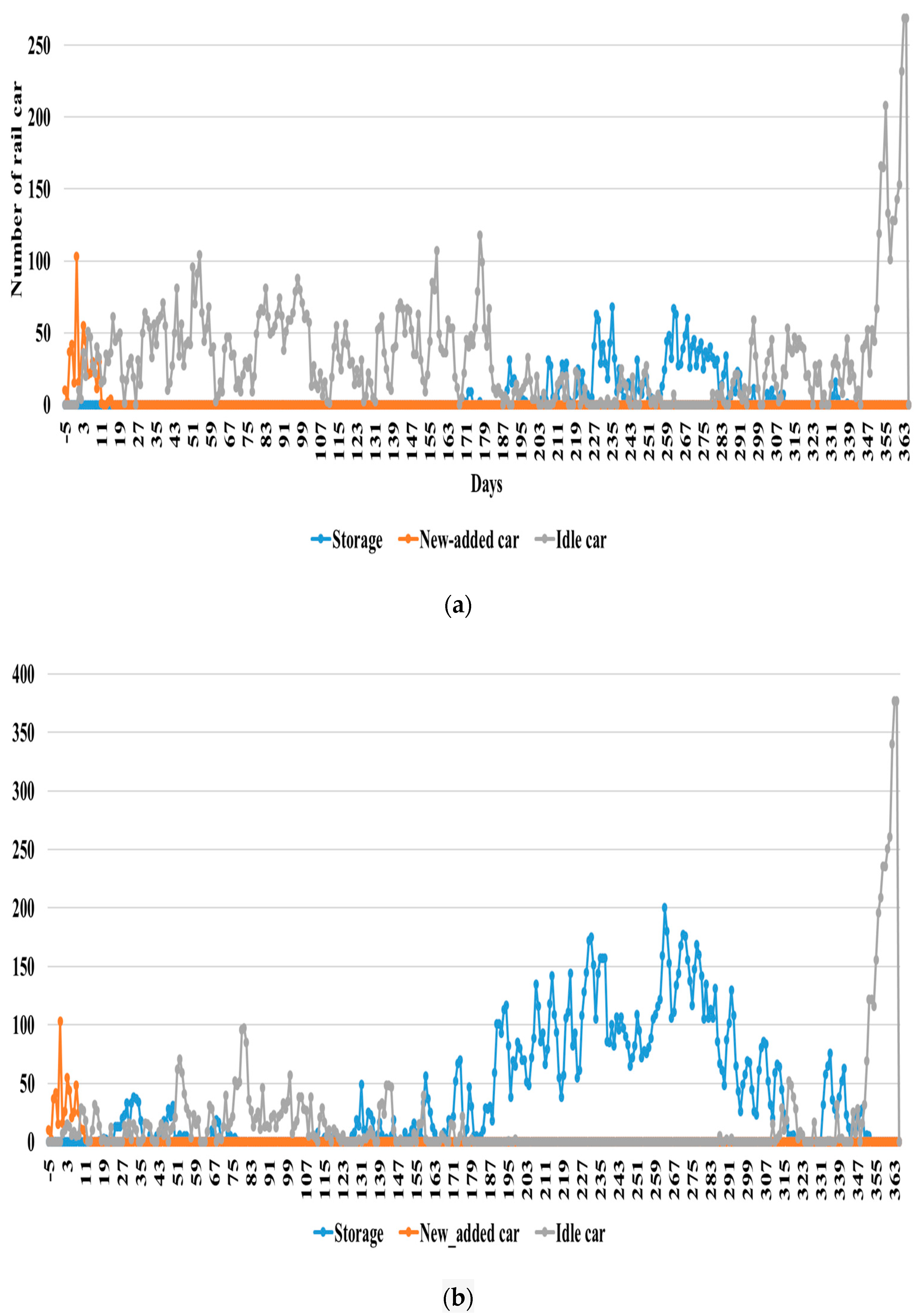
Figure 5 and
Figure 6 show the results of the four alternatives under Scenario 2 in graphical format. Both Figures show the amounts of logs that required storage (in carloads), as well as the number of added and idled rail cars per day. All the alternatives had some idled cars (mainly in the spring) and some storage (summer and fall). As expected, Alternative 1 (
Figure 5a) with a larger car fleet and quicker loading/unloading see much less storage and more idling than the other alternatives, especially Alternative 4 (
Figure 6b) which has a smaller fleet and longer loading/unloading times. Under Alternative 4, car idling is almost eliminated (except at the end of year, as the simulation was not continued to the next year).
To better understand the need for storage with different alternatives, we calculated the percentage of car loads stored, as well as the average storage days at the origin sites (
Table 6). The table shows that a one day increase in unloading and loading time results in a double-digit increase in stored loads and almost doubles the average days spent in storage. We can also see that the results for Alternative 2 and 3 are very close. This suggests that the storage impact of one added day in the loading/unloading process equals the removal of almost 100 cars from the fleet rotation. We also found that 400 car rotation would eliminate idling, but 31–47% of logs would be stored (Alternatives 3 and 4), depending on the loading/unloading time. In Alternatives 3 and 4, the average storage time was 3–5 days, but we found a great variation between individual sidings. For example, under Alternative 4 the storage days (average 5.3) ranged from 2.8 days (Gulliver, MI, USA) up to 25.1 days (Crivitz, MI, USA).
5. Discussion and Conclusions
The availability of rail transportation for log movements in the Upper Midwest region of the US is considered essential to maintaining the economic health of the industry, as well as reducing the environmental and social impacts from large log trucks. As rail traffic has dwindled and an increasing portion of existing rail car fleet is reaching the end of its service life, neither shippers nor railroads have had a clear understanding of what fleet size would meet the demands in the region and maintain rail as a sustainable alternative for the industry.
One fleet replacement alternative is the formation of a dedicated fleet of rail cars shared by all industry companies in the region. We used actual log shipment and train movement data to develop ILP models for estimating the size of shared rail car fleet needed to move the current log volumes. While the analyses conducted were hypothetical (we have only a part of the actual rail car routing data), they were based on true data and provide a solid foundation for future activities in the region, whether they relate to fleet size determinations or to the efficiencies in car circulation.
The analysis revealed that approximately 400–600 dedicated log cars, depending on the specific month, would be able to move the logs without any temporary storage at the origin. This would remove all excess empty kilometers by cars and provide the fastest circulation possible, but it would also require that each car in the fleet be immediately moved to the nearest location needing a car after unloading (independent of the company in need of service). If the high end of fleet size were available for the whole year (593 cars), logs could always move forward in timely fashion, but on average 25 cars (5% of the fleet) would be idling on any given date.
We also investigated how variations in the fleet size and loading/unloading times would impact the temporary storage need for logs at the origin site. We were able to almost eliminate the car idling by reducing the fleet size to 400, but 31–47% of loads would have to be stored on average for 3.0–5.3 days, depending on the loading/unloading time. This would be the preferred situation from the rail operator perspective, as the cars only provide revenue when moving with logs. On the other hand, it would require temporary storage of logs at the siding, both elements that increase the costs for shippers. With 493 cars and 1.5 days of loading/unloading, only eight percent of the loads would have to be stored, but this would increase to almost 30 percent if loading/unloading were each increased by a day. The analysis under Scenario 2 also revealed that a reduction of a single day in the loading/unloading process (2.5 to 1.5 days), would eliminate almost 100 cars (20%) from the fleet without a reduction in throughput, suggesting that opportunities for processing time reductions are a noteworthy strategy to look into in the future.
While the study received unprecedented support from shippers and rail carriers, there were certainly limitations that should be recognized when interpreting the results. For example, the car peaking and fleet size analysis used ideal conditions with no consideration for foul weather or equipment-related delays. In reality, both weather and equipment issues are likely to create some uncertainty in the results and should be accounted for in the actual fleet size. These stochastic considerations will be included in the next phases of the research, but to maintain the high level of accuracy of our analysis, we will collect detailed industry data on weather-related delays, equipment-related failure rates, and the frequencies and durations of maintenance activities.
In addition, the analysis considered all cars to belong to a single equipment pool shared by all the companies and mills. In reality, some cars are privately owned and their routes are limited to the controlling company, reducing the opportunities to optimize fleet circulation. We believe that one option to address this shortcoming in future research is through bilevel programming to analyze how decisions by one party (the administrator of the pool) or by the rail service provider impact the needs by any individual companies using the pool resources. However, we also recognize that some of the necessary data for these analyses may be inaccessible due to data confidentiality.
Author Contributions
The authors confirm contribution to the paper as follows: Conceptualization, S.K. and P.L.; Methodology, S.K. and K.Z.; Software, S.K. and K.Z.; Validation, S.K., P.L. and K.Z.; Formal Analysis, S.K.; Investigation, S.K. and P.L.; Data collection, S.K. and P.L.; Writing—Original Draft Preparation: S.K.; Writing—Review & Editing, S.K., P.L. and K.Z.; Project Administration, P.L.; Funding Acquisition, P.L. All authors reviewed the results and approved the final version of the manuscript.
Funding
This research was funded by the Michigan Economic Development Corporation (MEDC), the Michigan Department of Transportation (MDOT), and the US DOT OST-R Tier 1 University Transportation Center, DTRT12-G-UTC18/DTRT13-G-UTC52. Additionally, the APC and the promotional activities of this research were funded by a grant from R&D program of the Korean Railroad Research Institute, Korea.
Acknowledgments
The research team would like to acknowledge the forest product companies associated with LSSA and two rail carriers (CN and E&LS) who supported the research.
Conflicts of Interest
The authors declare no conflict of interest. The founding sponsors had no role in the design of the study; in the collection, analyses, or interpretation of data; in the writing of the manuscript, and in the decision to publish the results.
References
- Song, Y.; Liu, Z.; Rønnquist, A.; Nåvik, p.; Liu, Z. Contact Wire Irregularity Stochastics and Effect on High-speed Railway Pantograph-Catenary Interactions. IEEE Trans. Instrum. Meas. 2020. [Google Scholar] [CrossRef]
- Goverde, R.M. Punctuality of Railway Operations and Timetable Stability Analysis. Ph. D. Thesis, Delft University of Technology, Delft, The Netherlands, 2005. [Google Scholar]
- Pouryousef, H.; Lautala, P. Hybrid simulation approach for improving railway capacity and train schedules. Plan. Manag. 2015, 5, 211–224. [Google Scholar] [CrossRef]
- Antich, M. Why Railcar Constraints Continue to Impact Order-to-Delivery. In Automotive Fleet; Bobit Business Media: Torrance, CA, USA, 2019. [Google Scholar]
- Transportation, S.F. A Comparison of the Costs of Road, Rail, and Waterways Freight Shipments That Are Not Passed on to Consumers; 2013, GAO-11-134; US Government Accountability Office: Washington, DC, USA, 2011.
- Sherali, H.D.; Maguire, L.W. Determining rail fleet sizes for shipping automobiles. Interfaces 2000, 30, 80–90. [Google Scholar] [CrossRef]
- Bojović, N.J. A general system theory approach to rail freight car fleet sizing. Eur. J. Oper. Res. 2002, 136, 136–172. [Google Scholar] [CrossRef]
- Sayarshad, H.R.; Ghoseiri, K. A simulated annealing approach for the multi-periodic rail-car fleet sizing problem. Comput. Oper. Res. 2009, 36, 1789–1799. [Google Scholar] [CrossRef]
- Yaghini, M.; Khandaghabadi, Z. A hybrid metaheuristic algorithm for dynamic rail car fleet sizing problem. Appl. Math. Model. 2013, 37, 4127–4138. [Google Scholar] [CrossRef]
- Milenković, M.; Bojović, N. A fuzzy random model for rail freight car fleet sizing problem. Transp. Res. Part C Emerg. Technol. 2013, 33, 107–133. [Google Scholar] [CrossRef]
- Bachkar, K.; Awudu, I.; Osmani, A.; Hartman, B.C. Fleet management for rail car transport of ethanol. Res. Transp. Bus. Manag. 2017, 25, 29–38. [Google Scholar] [CrossRef]
- White, W.W.; Bomberault, A.M. A network algorithm for empty freight car allocation. IBM Syst. J. 1969, 8.2, 147–169. [Google Scholar] [CrossRef]
- Joborn, M.; Crainic, T.G.; Gendreau, M.; Holmberg, K.; Lundgren, J.T. Economies of scale in empty freight car distribution in scheduled railways. Transp. Sci. 2004, 38, 121–134. [Google Scholar] [CrossRef]
- Narisetty, A.K.; Richard, J.P.P.; Ramcharan, D.; Murphy, D.; Minks, G.; Fuller, J. An optimization model for empty freight car assignment at Union Pacific Railroad. Interfaces 2008, 38, 89–102. [Google Scholar] [CrossRef]
- Heydari, R.; Melachrinoudis, E. A path-based capacitated network flow model for empty railcar distribution. Ann. Oper. Res. 2017, 253, 773–798. [Google Scholar] [CrossRef]
- Kallrath, J.; Klosterhalfen, S.T.; Walter, M.; Fischer, G.; Blackburn, R. Payload-based fleet optimization for rail cars in the chemical industry. Eur. J. Oper. Res. 2017, 259, 113–129. [Google Scholar] [CrossRef]
- LSSA. Lake States Shippers Association-Web Page. 2019. Available online: http://www.centralcorridors.com/lssa/index.html (accessed on 30 October 2019).
- DOT, U.S. Transportation Networks; National Transportation Atlas Database; Bureau of Transportation Statistics: Washington, DC, USA, 2016.
- IBM. Branch & cut or dynamic search? IBM Knowledge Center 2017. Available online: https://www.ibm.com/support/knowledgecenter/pl/SSSA5P_12.7.1/ilog.odms.cplex.help/CPLEX/UsrMan/topics/discr_optim/mip/performance/13_br_cut_dyn_srch.html (accessed on 15 December 2017).
- Danna, E.; Rothberg, E.; Le Pape, C. Exploring relaxation induced neighborhoods to improve MIP solutions. Math. Program. 2005, 102, 71–90. [Google Scholar] [CrossRef]
- IBM. CPLEX User’s Manual; Version 12 Release 7; IBM ILOG CPLEX Optimization Studio: New York, NY, USA, 2016. [Google Scholar]
© 2020 by the authors. Licensee MDPI, Basel, Switzerland. This article is an open access article distributed under the terms and conditions of the Creative Commons Attribution (CC BY) license (http://creativecommons.org/licenses/by/4.0/).


