Assessing the Impacts of Urban Expansion on Habitat Quality by Combining the Concepts of Land Use, Landscape, and Habitat in Two Urban Agglomerations in China

Abstract

Understanding the spatiotemporal variability of habitat quality as a function of land-use changes is important for expanding scientific knowledge of ecological conservation. In this study, the impacts of land-use change on habitat quality were assessed in two urban agglomerations in China at different stages of development, namely (1) the Yangtze River Delta Urban Agglomeration (YRDUA), which has reached the middle and late stage of urbanization, and (2) the Golden Triangle of Southern Fujian (GTSF), which has reached the middle and early stage. The Integrated Valuation of Ecosystem Services and Tradeoffs (InVEST) habitat quality model was applied to determine the habitat quality and the degree of habitat degradation in these two agglomerations. Overall, the habitat quality in the YRDUA was found to be clearly inferior to that in the GTSF. In the GTSF, more than 65% of the habitat was of good or excellent quality, whereas in the YRDUA, less than 45% of the habitat reached this quality. By combining the concepts of land use, landscape, and habitat, the boundary of degradation and the general increase in habitat quality from 2000 to 2015 were found to be mainly related to the landform, the dominant landscape, and the concentration of non-habitat areas. Additionally, the type, distribution, and fragmentation of the dominant habitat were shown to play important roles in habitat quality. Moreover, changes in industrial composition over time were demonstrated to be critical drivers of changes in areas of construction land.

1. Introduction

Overall, 55% of the world’s population resided in urban areas in 2018. By 2050, this is projected to increase to 68% [1]. Due to urbanization and concomitant population aggregation, cities are experiencing inevitable expansion. With the attractions of some big cities and the help of convenient transport, flows of materials, energy, and information are occurring with increasing frequency, and the interactive effects between them are getting bigger and bigger. Urban growth, accompanied by ecological and environmental problems, exhibits significant agglomeration effects [2,3,4].

In 1957, Jean Gottmann chose the word “Megalopolis” to describe a vast region of adjacent urban areas that have become increasingly fused over time into what could be conceived as a super city [5]; hence the origin of urban agglomeration. The emergence and development of urban agglomerations leads to drastic land-use changes, thus greatly impacting the supply of ecosystem services [6]. There are three main ways that land-use change affects ecosystem services: (1) It directly affects the spatial and temporal distribution of biological habitats and resources, and thus changes the spatiotemporal pattern of the generation, delivery, and expression of ecosystem services [7,8]; (2) It also affects ecosystem services by changing biodiversity, such as by varying the characteristics of plants [9] or changing plant functional diversity [10]; (3) It also has direct effects on ecosystem services themselves by changing ecosystem processes, such as hydrological processes [11] and the recycling of organic matter and nutrients [12].

Integrated Valuation of Ecosystem Services and Tradeoffs (InVEST) is a set of effective models that is used to quantify and visualize ecosystem services in conjunction with Geographic Information System (GIS) software [13,14]. Essentially, the patterns in the production of ecosystem services are spatial, and such patterns can be estimated via the analysis of land-use/land-cover (LULC) maps. Thus, InVEST models can be used to explore what kind of evolution in terrestrial ecosystems may bring beneficial changes to human beings. For example, these models can be employed to undertake a quantitative evaluation of the spatially heterogeneous ecological benefits of soil conservation [15,16], to calculate forest carbon stocks and monitor the temporal dynamics of these stocks [17,18], or to study the effects of land-use changes on habitat quality [19,20]. Due to the high concentration of human activities in urban ecosystems, the magnitudes and spatial patterns of all types of ecosystem services have been severely affected [21]. Previous studies have evaluated urban ecosystem services based on InVEST models. These not only include comprehensive evaluations of the impacts of human activities and urban development on various types of ecosystem services [22,23] but also evaluations of the impacts of urban expansion on certain types of ecosystem service, such as carbon storage [24,25,26], soil conservation [27], and habitat quality [28].

Habitat quality refers to the ability of an ecosystem to provide the conditions appropriate for individual and population persistence. InVEST models habitat quality as one of the proxies for biodiversity, which is intimately linked to the production of ecosystem services [13]. In other words, the InVEST habitat quality model combines information on LULC and threats to biodiversity. The objective of this study was to assess the impacts of land-use change on habitat quality in two urban agglomerations in China at different stages of development, namely the Yangtze River Delta Urban Agglomeration (YRDUA) and the Golden Triangle of Southern Fujian (GTSF). According to the national urban hierarchical plan compiled by the China Academy of Urban Planning and Design, the YRDUA is a world-class urban agglomeration and the GTSF is a second-class urban agglomeration that is an important part of the Western Taiwan Straits Economic Zone. As such, development patterns in the YRDUA could serve as a reference for the development of the GTSF.

2. Study Area and Data Sources

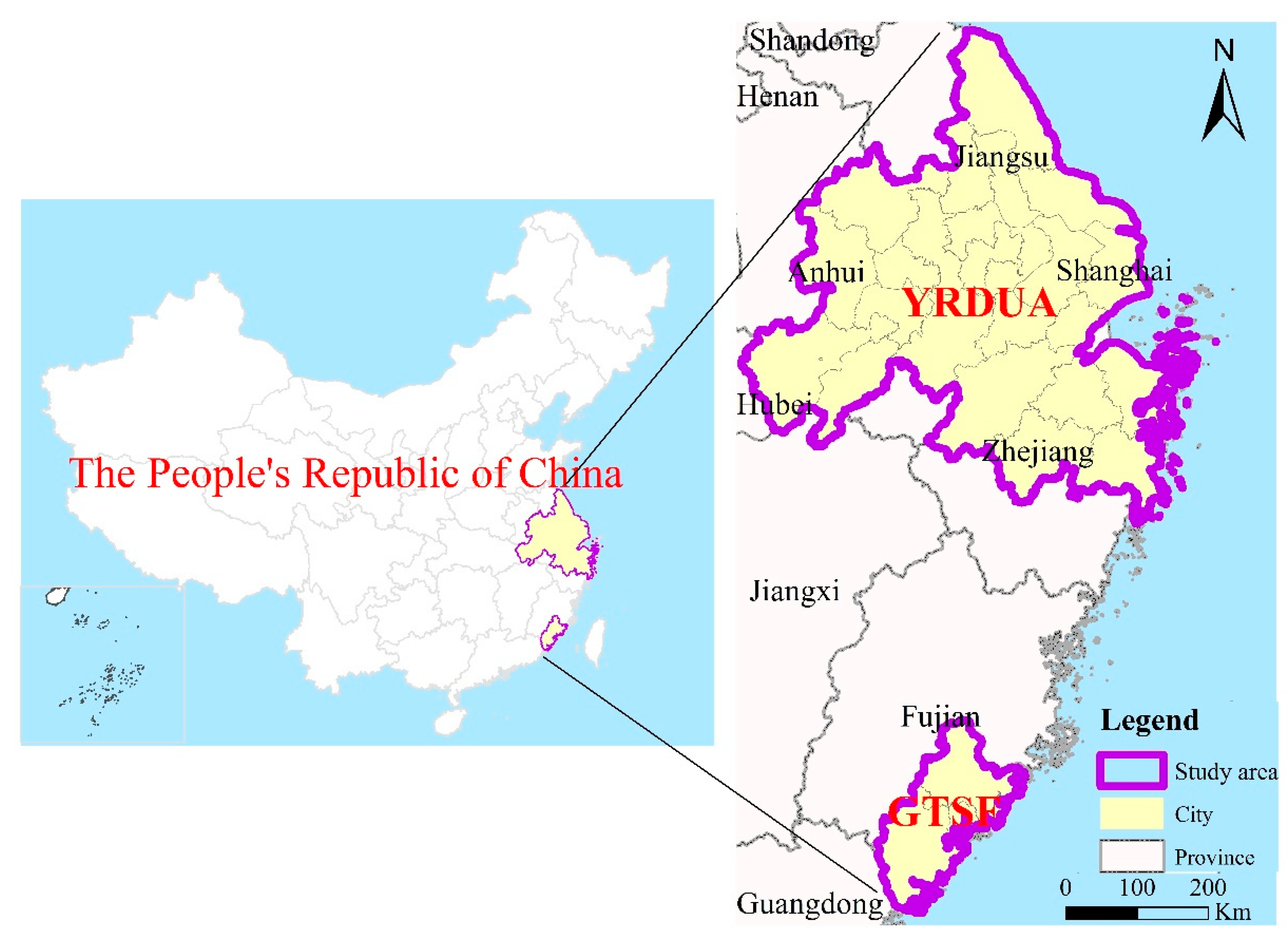
2.1. Study Area

The YRDUA is located in the coastal area of the Yangtze River Estuary [29] and is one of the most developed, densely populated, and industrially concentrated areas in China. Since the YRDUA has developed into one of six influential world-class metropolises, it has become increasingly important to China’s economic and social development [30]. The boundaries of the YRD are different when considering different factors; for example, cultural, economic, or geographical. The Yangtze River Delta Urban Agglomeration development plan (2015–2030) issued by the State Council of China in May 2016 stated that the YRDUA covered a total of 26 cities: Shanghai plus nine cities in Jiangsu Province, eight cities in Zhejiang Province, and eight cities in Anhui Province. For the purposes of defining the sampling frame of this study, the latest official region of the YRDUA is used (Figure 1), which covers an area of 211,700 square kilometers, accounting for about 2.2% of the country’s total area [31].

The GTSF is a region constituted by the cities of Xiamen, Quanzhou, and Zhangzhou. The GTSF is a rapidly growing urban area in the southeast of Fujian Province, on the southeastern coastline of China [32]. With an area of about 25,000 square kilometers, it accounts for 20.7% of the total area of Fujian Province and generates 40% of the province’s gross domestic product [33]. Following China’s reform and opening-up, the GTSF has become one of the most economically developed regions in the country. Although the GTSF cannot be compared with more economically developed regions such as the Pearl River Delta and the Yangtze River Delta, this area has nevertheless attracted a large amount of investment from Taiwan due to its unique geographical location, language environment, and customs.

The reasons for choosing these two study areas are as follows: Firstly, the coastal area of China is an area of concentrated industrialization and urbanization that is typically used as a research area. Secondly, the YRDUA is densely populated, industrially concentrated, and highly urbanized, and the GTSF is in a stage of rapid urbanization and has wealthy and abundant natural resources. Thirdly, the comparative analysis of these two study areas will help to reveal the impact of urbanization on the environment and provide support for habitat protection under rapid urbanization.

2.2. Data Sources

LULC maps of the two case-study regions for the period 2000–2015 were downloaded from the multi-temporal land-use database on the Resource and Environment Data Cloud Platform (http://resdc.cn 5a, four scenarios). The database covers the whole of China and has been established after years of accumulation under the support of many major research projects. The Landsat TM/ETM+ remote sensing imagery (30 m × 30 m resolution) was used as the main data source to produce the dataset, which was generated manually based on visual interpretation using a classification system shown in

Table 1. Land-use classification system.

Class1	Class2	Class1	Class2
Farmland	Paddy field	Wetland	River
	Dryland		Lake
Forest	Woodland		Reservoir
	Shrubwood		Tidal flat
	Sparse forest		Beach
	Other woodland		Marshland
Grassland	High-coverage grassland		Sea
	Moderate-coverage grassland	Construction land	Urban land use
	Low-coverage grassland		Rural residential areas
Bare land	Bare land		Other construction land
	Bare rock

. This system is a classification system of land-use types divided into six primary and 21 secondary classes (Table 1). Statistical data were collected from the Yearbooks of 29 cities in the period 2000–2015 (5a).

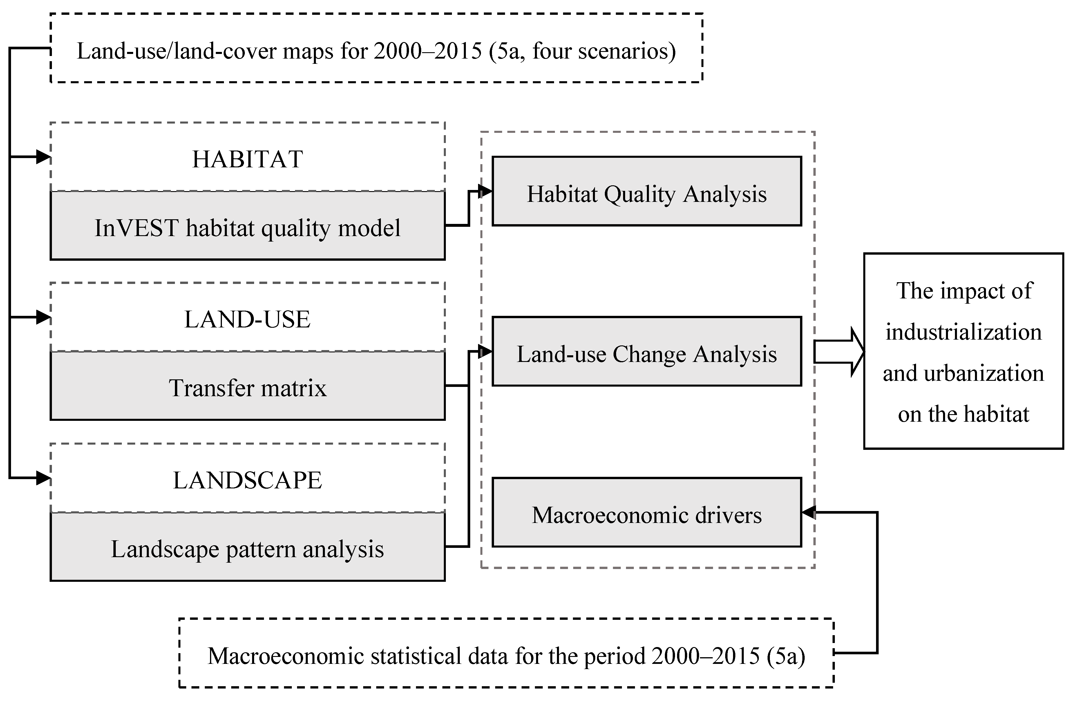
3. Methodological Approach

Based on the LULC maps of the two case-study regions for the period 2000–2015 (5a, four scenarios), habitat quality and land-use change were analyzed using the InVEST habitat quality model and transfer matrix and landscape pattern analysis, respectively, according to the habitat, land use, and landscape. By combining the concepts of habitat, land use, and landscape, the macroeconomic drivers were then introduced to study the impacts of urbanization and industrialization on the habitat. The framework of the methodological process is shown in Figure 2.

3.1. Land-Use Change Analysis

To uncover and understand the interrelations between urban land-use changes and habitat quality, spatial features and temporal processes had to be jointly analyzed. Firstly, the amount of land-use change in the Yangtze River Delta and the Golden Triangle of Southern Fujian was calculated. Next, a transfer matrix was applied to study variations across all types of land use. Then, using the Fragstats version 4.1 software package, particular landscape metrics were selected to analyze the characteristics of landscape patterns based on class-and landscape-level considerations (

Table 2. Description of landscape metrics.

Landscape Metrics	Level	Significance
NP	Class/Landscape	The higher the NP, the higher the degree of fragmentation.
PD	Class/Landscape	The number of patches per unit area; the higher the PD, the higher the degree of fragmentation.
AREA_MN	Class/Landscape	Represents an average situation; patches with smaller values are more fragmented than those with larger values.
LPI	Class	Reflects the dominant type. In one landscape type, the ratio of the largest patch to the total landscape area.
COHESION	Class	The aggregation degree of a landscape type; the higher the COHESION, the higher the degree of aggregation.
CONTAG	Landscape	The higher the value, the better the connectivity.
DIVISION	Landscape	The segmentation degree of a landscape type with different patch numbers.
LFI	Class/Landscape	Represents the degree of fragmentation of the landscape and the complexity of landscape spatial structure.

NP: Number of Patches; PD: Patch Density; AREA_MN: Mean Patch Area; LPI: Largest Patch Index; COHESION: Patch Cohesion Index; CONTAG: Contagion; DIVISION: Landscape Division Index; LFI: Landscape Fragmentation Index, LFI = (NP − 1)/AREA_MN.

). The representative significance of all these eight landscape metrics was categorized into four types, namely the fragmentation, the aggregation, the connectivity, and the dominant type [20,28]. For example, the higher the Number of Patches (NP) or Patch Density (PD) metrics, the higher the degree of fragmentation, while the higher the Patch Cohesion Index (COHESION) metric, the higher the degree of aggregation.

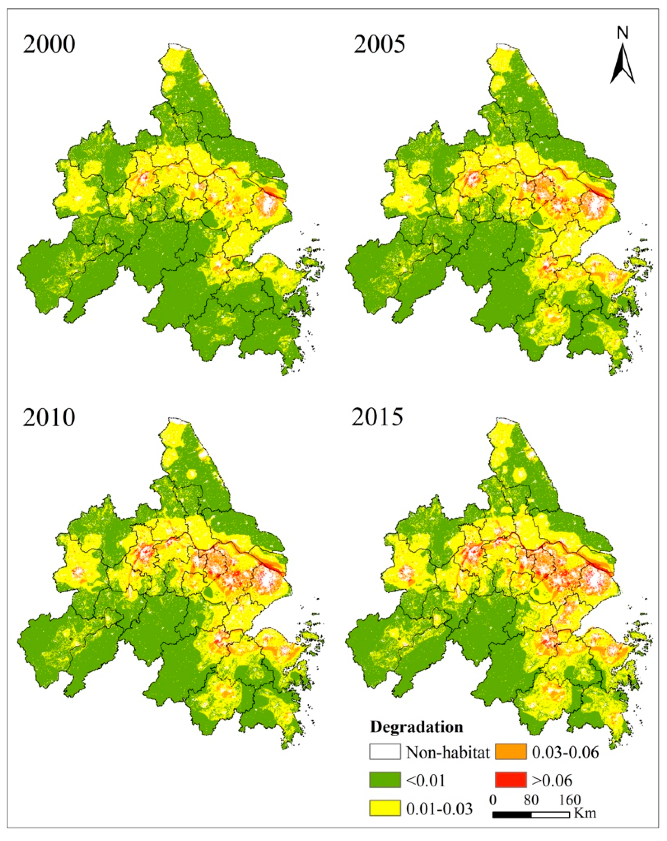
3.2. Habitat Quality Analysis

Combining the information from the LULC maps and the habitat threats of biodiversity, the InVEST habitat quality model was used to generate habitat quality maps that contained the degradation degree and the habitat quality score of all land-cover types in one particular region. Being considered as a continuous variable in this model, habitat quality ranges from low, through medium, to high [34]. High-quality habitats are relatively intact in terms of their structure and stable in terms of their function within a certain period. Generally, habitat quality depends on the proximity of habitats to human land uses and the intensity of these land uses, and the degradation of habitats depends on the intensity of nearby land use [35,36,37].

Habitat quality is based on the following four factors: (1) The relative impact among the threats, (2) the distance between the habitat and the threat and the impact from the threat, (3) the level at which a grid cell of the habitat is legally/socially/physically protected, and (4) the relative sensitivity of each habitat to each threat. Therefore, the habitat quality in grid cell x in habitat type or LULC type j is given by $Q_{xj}$ (Equation (1)):

$$Q_{xj}=H_j\left[1-\left(\frac{D_{xj}^z}{D_{xj}^z+k^z}\right)\right]$$

(1)

where $H_j$ indicates the habitat suitability of LULC type j; $D_{xj}$ is the total threat level; k is the half-saturation value, which is equal to half of the peak value of $D_{xj}$; and z is a normalized constant, which is fixed at 2.5.

The most significant aspect of the habitat approach is the ability to characterize the sensitivity of habitat types to diverse threats. Not all habitats are influenced by threats in the same way. For example, forest could be more sensitive to the threat of urban land use than rural residential areas. The model also incorporates the distance over which a threat will bring degradation to natural systems. Because human activities are mostly concentrated in areas of construction land, three secondary classes of construction land are taken as the threats in this study. Moving onto habitat sensitivity to threats, at the extremes, we treat forest as habitat and bare land as non-habitat. Being the most sensitive habitat type, forest is more sensitive to rural residential areas or other construction land than is urban land use (0.8 and 0.8 versus 0.9 in the GTSF). The threat factor properties of these three classes of construction land are shown in

Table 3. Threat factor properties.

Threat	Max Dist	Weight	Decay
Urban land use	10	1	Exponential
Rural residential areas	5	0.5	Exponential
Other construction land	10	0.7	Exponential

Note: Threat: the name of the specific threat; MAX_DIST: the maximum distance over which each threat affects habitat quality (measured in km) so that the impact of each degradation source declines to zero at this maximum distance; Weight: the impact of each threat on habitat quality, relative to other threats, ranging from 0 to 1; Decay: the functional form of decay over space associated with the threat, either “linear” or “exponential”.

, and the sensitivities of other habitat types to each threat are shown in

Table 4. The sensitivity of habitat types to each threat factor.

Land Use Type	Habitat	YRDUA			GTSF
		L_urbl	L_rra	L_ocl	L_urbl	L_rra	L_ocl
Paddy field	0.5	0.35	0.35	0.3	0.3	0.3	0.3
Dryland	0.3	0.3	0.3	0.2	0.3	0.3	0.2
Woodland	1	0.85	0.75	0.75	0.9	0.8	0.8
Shrub wood	1	0.85	0.75	0.75	0.9	0.8	0.8
Sparse forest	0.8	0.85	0.75	0.75	0.9	0.8	0.8
Other woodland	0.8	0.5	0.5	0.5	0.9	0.8	0.8
High-coverage grassland	0.7	0.5	0.35	0.5	0.6	0.3	0.6
Moderate-coverage grassland	0.6	0.5	0.35	0.5	0.5	0.3	0.5
Low-coverage grassland	0.5	0.5	0.35	0.5	0.5	0.3	0.5
River	0.8	0.9	0.9	0.9	0.9	0.9	0.9
Lake	0.9	0.9	0.9	0.9	0.9	0.9	0.9
Reservoir	0.8	0.8	0.8	0.8	0.8	0.8	0.8
Tidal flat	0.7	0.75	0.8	0.8	0.8	0.8	0.6
Beach	0.7	0.75	0.8	0.8	0.8	0.8	0.6
Marshland	0.9	0.9	0.8	0.8	0.9	0.9	0.9
Sea	0	0	0	0	0	0	0
Urban land use	0	0	0	0	0	0	0
Rural residential areas	0	0	0	0	0	0	0
Other construction land	0	0	0	0	0	0	0
Bare land	0	0	0	0	0	0	0
Bare rock	0	0	0	0	0	0	0

Note: L_urbl, L_rra and L_ocl: The relative sensitivity of each habitat type to each threat (urban land use, rural residential areas and other construction land). The sensitivity of the Golden Triangle of Southern Fujian was mainly based on reference [20], and the sensitivity of the Yangtze River Delta Urban Agglomeration was based on references [38,39,40,41,42].

. These are value-assigned based on the extant literature [20,28,38,39,40,41,42] and the opinions of some experts.

3.3. Macroeconomic Drivers Analysis

Some researchers consider that, in a short period, changes in landscape patterns are mainly due to the influence of social and economic factors. We directly quote the conclusions of relevant studies [43,44,45,46]; for example, that there is a positive correlation between GDP and the area of construction land, and GDP is the sum of the added value of primary, secondary, and tertiary industries. In this study, by combining the concepts of land use, landscape, and habitat, we introduce macroeconomic drivers to further explain the reasons for the changes of habitat quality.

4. Results

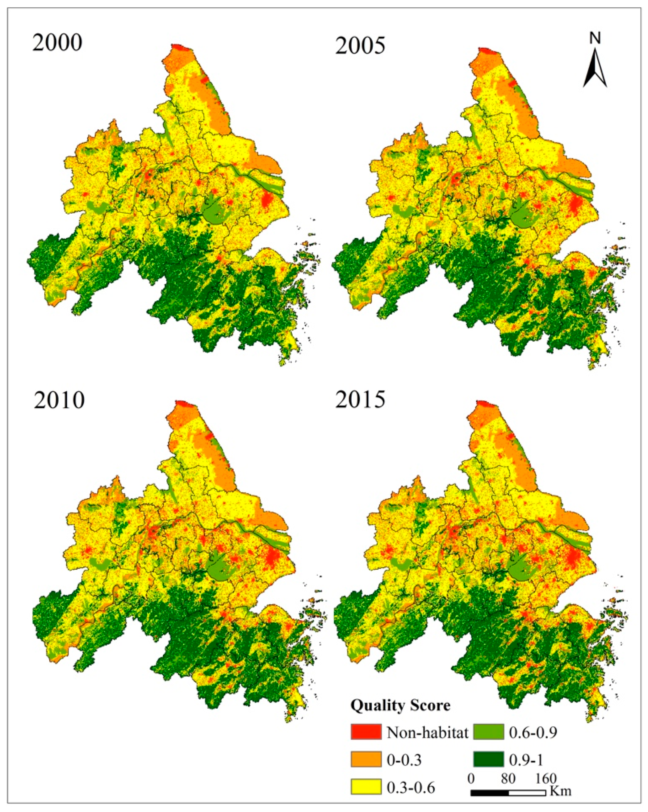
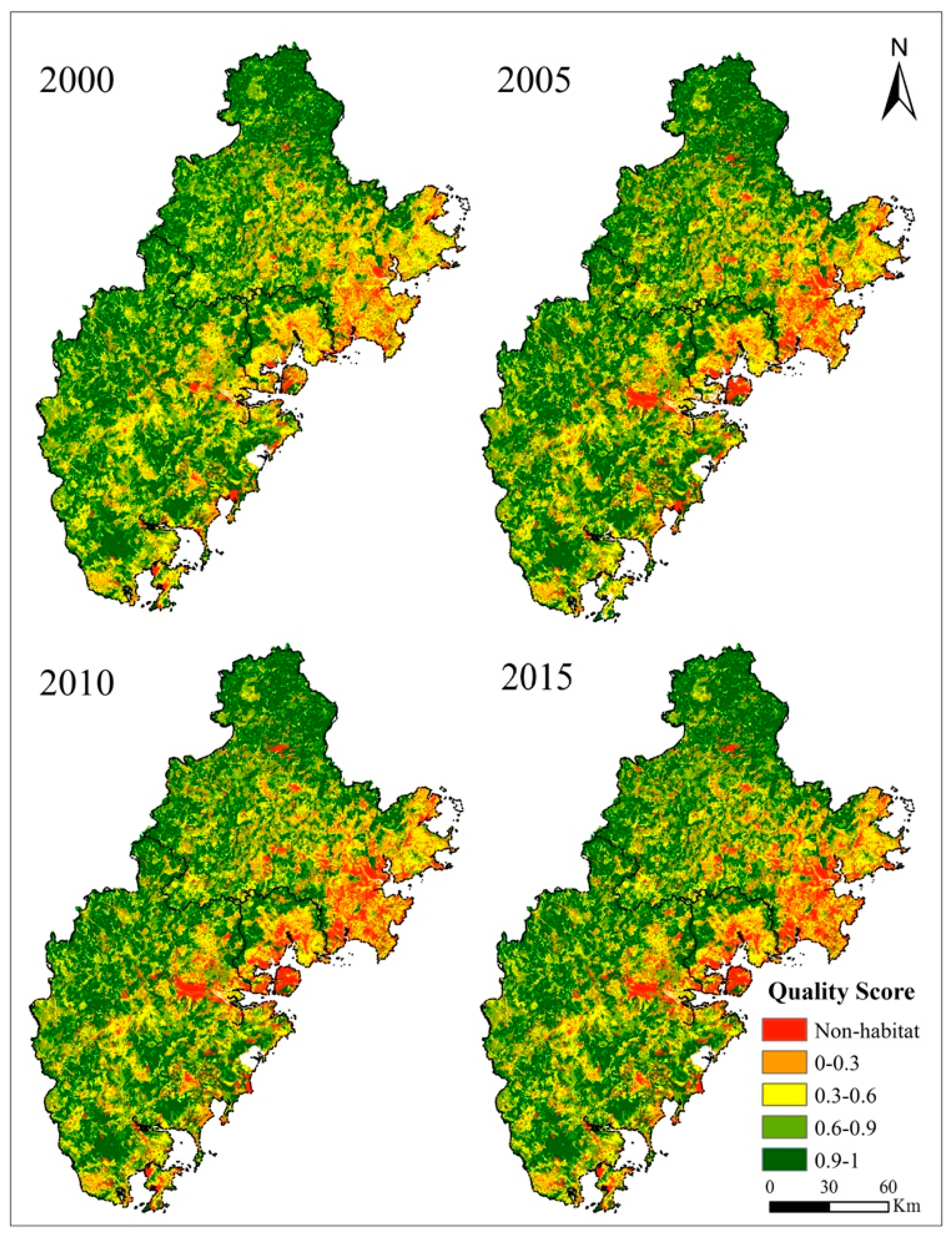
4.1. Habitat Quality Analysis

Upon execution of the InVEST habitat quality model, results were generated pertaining to the relative level of habitat degradation and habitat quality during the period 2000–2015 for the two urban agglomerations.

Grid cells with non-habitat land cover are assigned a degradation score of 0; a higher score means more severe degradation. The spatial distributions of habitat degradation in the two urban agglomerations are shown in Figure 3 and Figure 4. Since construction land was the main non-habitat land cover, habitat degradation centered on those non-habitats and proceeded outwards along rivers. Furthermore, with the expansion of the two urban agglomerations from 2000 to 2015, the boundaries of habitat degradation exhibit an obvious outward-migration trend over time.

Habitat quality scores vary continuously between 0 and 1 on the raster layer. The non-habitat land cover areas are assigned a value of 0; a higher value indicates better habitat quality. The spatial distributions of habitat quality in the two urban agglomerations are shown in Figure 5 and Figure 6. Habitat quality in the YRDUA exhibited a decreasing trend from south to north, and a near-identical decreasing trend from southwest to northeast in coastal areas was observed in the GTSF. Overall, coastal areas tended to exhibit low scores whilst the scores of first-tier cities in these urban agglomerations were usually below 0.6. It was particularly apparent that there were large and continuous areas with low scores in the downtown areas of these first-tier cities.

For better comparison and illustration, by using the geometric interval classification method in the ArcGIS software, the habitat quality results in each period were divided into four intervals—namely 0–0.3, 0.3–0.6, 0.6–0.9, and 0.9–1—corresponding, respectively, with the four valuation levels of low, medium, good, and excellent. The proportion of habitat in each quality interval was then calculated (

Table 5. Changes in habitat quality over time in the YRDUA and GTSF.

Valuation Level	Value Interval	YRDUA				GTSF
		2000	2005	2010	2015	2000	2005	2010	2015
Low	[0,0.3)	10.42%	10.49%	10.47%	10.58%	9.68%	9.44%	9.23%	9.21%
Medium	[0.3,0.6)	46.98%	46.14%	45.65%	45.15%	25.36%	24.34%	23.85%	23.63%
Good	[0.6,0.9)	15.32%	15.74%	16.04%	16.19%	22.63%	22.96%	23.67%	23.88%
Excellent	[0.9,1]	27.28%	27.63%	27.84%	28.08%	42.33%	43.26%	43.25%	43.29%

). Overall, it was found that the habitat quality in the Yangtze River Delta was clearly inferior to that of the Golden Triangle of Southern Fujian. In the GTSF, more than 65% of the habitat was of good or excellent quality. Meanwhile, in the YRDUA, 45% of the habitat was of medium quality, with lower proportions registered for the other quality intervals. From 2000 to 2015, the proportion of habitat of medium and low (good) quality decreased (increased) in the YRDUA and GTSF year by year. Temporal changes in excellent habitat were less apparent, although there was a slightly decreasing (increasing) trend in the GTSF (YRDUA).

4.2. Changes in Habitat Quality Induced by Land-Use Changes

Between 2000 and 2015, the area of bare land in the YRDUA increased by 17.21 km². Compared with the total land area of the YRDUA, the area of bare land is very small, and its growth rate was 58.57%. Meanwhile, the total area of bare land in the GTSF is small, and its area was basically unchanged between 2000 and 2015. During this period, the area of construction land increased greatly in the YRDUA and GTSF, with the area increasing by 8539.24 km² and 1199.24 km², respectively, with maximum increases of 63.82% and 94.23%, respectively. The farmland area decreased by 7964.67 km² and 824.47 km² in the YRDUA and GTSF, respectively, representing decreases of 7.01% and 12.94%, respectively. In the YRDUA, the area of forest decreased by 1.52%, while the areas of grassland and wetland increased by 2.71% and 2.94%, respectively. In the GTSF, the areas of forest and grassland decreased by 2.84% and 3.16%, respectively, and the area of wetland increased by 32.10%.

A land-use transfer matrix was used to analyze losses of all types of land use (

Table 6. Land-use transfer matrix for the YRDUA (Unit: %).

Year	LULC	Bare Land	Wetland	Construction Land	Grassland	Farmland	Forest
2000–2015	Bare land	-	9.12	2.49	0.00	0.38	4.90
	Wetland	0.00	-	2.09	0.74	4.12	0.26
	Construction land	0.01	0.39	-	0.11	5.01	0.14
	Grassland	0.02	1.12	1.05	-	1.74	2.10
	Farmland	0.01	1.18	7.29	0.09	-	1.07
	Forest	0.01	0.14	0.86	0.59	2.44	-
2000–2005	Bare land	-	0.00	5.24	0.00	0.49	0.00
	Wetland	0.00	-	0.68	0.10	1.66	0.07
	Construction land	0.00	0.16	-	0.01	2.12	0.05
	Grassland	0.01	0.37	0.33	-	0.72	0.31
	Farmland	0.00	0.62	2.95	0.01	-	0.20
	Forest	0.00	0.05	0.29	0.07	0.30	-
2005–2010	Bare land	-	0.11	0.00	0.00	0.05	3.13
	Wetland	0.00	-	0.49	0.01	0.36	0.01
	Construction land	0.00	0.07	-	0.00	1.64	0.03
	Grassland	0.00	0.17	0.19	-	0.04	0.04
	Farmland	0.00	0.18	2.27	0.01	-	0.10
	Forest	0.00	0.01	0.19	0.05	0.11	-
2010–2015	Bare land	-	8.95	0.16	0.01	0.35	1.91
	Wetland	0.00	-	1.19	0.69	3.22	0.28
	Construction land	0.01	0.41	-	0.12	5.98	0.30
	Grassland	0.03	0.64	0.55	-	1.01	1.86
	Farmland	0.01	0.60	3.21	0.08	-	0.93
	Forest	0.01	0.11	0.49	0.49	2.22	-

and

Table 7. Land-use transfer matrix for the GTSF (Unit: %).

Year	LULC	Bare Land	Wetland	Construction Land	Grassland	Farmland	Forest
2000–2015	Bare land	-	1.16	2.53	6.65	0.82	1.81
	Wetland	0.01	-	10.64	0.32	1.43	0.96
	Construction land	0.00	7.05	-	0.33	2.17	0.77
	Grassland	0.04	0.14	3.54	-	0.86	2.99
	Farmland	0.00	0.70	12.64	0.61	-	1.63
	Forest	0.01	0.14	2.61	1.06	0.80	-
2000–2005	Bare land	-	0.80	2.41	6.76	0.73	1.95
	Wetland	0.02	-	4.23	0.31	1.14	0.79
	Construction land	0.00	0.18	-	0.26	1.92	0.64
	Grassland	0.04	0.11	2.50	-	0.52	1.23
	Farmland	0.00	0.38	7.69	0.30	-	0.68
	Forest	0.01	0.09	1.93	0.36	0.42	-
2005–2010	Bare land	-	0.55	0.12	0.81	0.44	1.81
	Wetland	0.01	-	4.80	0.25	0.94	0.65
	Construction land	0.00	2.10	-	0.31	1.28	0.55
	Grassland	0.00	0.06	1.06	-	0.53	1.69
	Farmland	0.00	0.39	4.29	0.34	-	1.06
	Forest	0.00	0.08	0.69	0.71	0.38	-
2010–2015	Bare land	-	0.27	0.35	0.91	0.78	1.91
	Wetland	0.01	-	0.84	0.34	1.39	0.89
	Construction land	0.00	0.54	-	0.45	2.32	1.08
	Grassland	0.01	0.04	0.31	-	0.84	2.48
	Farmland	0.00	0.11	2.05	0.70	-	1.68
	Forest	0.00	0.04	0.22	0.75	0.77	-

). Although the rate of transformation of bare land and wetland was very high, in absolute terms the land areas in both cases are too small for analytical purposes. Thus, in the following, we focus on construction land (non-habitat) and farmland, forest, and grassland (habitats). The characteristic land-use change in the YRDUA and GTSF was the gradual expansion of construction land, which mainly occurred through the displacement of farmland. From 2000 to 2015, 7.29% and 12.64% of farmland changed to construction land in the YRDUA and GTSF, respectively. In terms of the reverse change, i.e., construction land to farmland, the figures were 5.01% and 2.17% for the YRDUA and GTSF, respectively. The transformations with respect to other habitats were not as sizeable as that between construction land and farmland. Interestingly, there was a net conversion of forest into farmland in the YRDUA, while the opposite was the case in the GTSF, where there was a net conversion of farmland into forest.

In the YRDUA, the transformation of other land to construction land was the main type of land-use change during the period from 2000 to 2010, while the conversion of other land to farmland and wetland was the main type from 2010 to 2015. In the GTSF, there were also two distinct transformation periods: From 2000 to 2010, the main type of transfer was from other land to construction land, grassland, and forest, while from 2010 to 2015, the main type was from other land to farmland and forest. Overall, these differential temporal trends explain why habitat quality increased over time in the YRDUA and GTSF.

Each terrain factor has a different degree of influence on land-use change; however, the elevation has a relatively greater impact [47]. The exploitation of land proceeds by first displacing flat areas, namely bare land, wetlands, or farmland [48]. Since the terrain of the two urban agglomerations is high in the east and low in the west, the habitat quality in coastal areas changed substantially between 2000 and 2015, and habitat degradation was also intensive along rivers during this time. Over two-thirds of the YRDUA is located on an alluvial plain, whereas the GTSF is relatively mountainous and hilly. As a result of its contiguous mountains, habitat quality in the GTSF was generally better than that in the YRDUA.

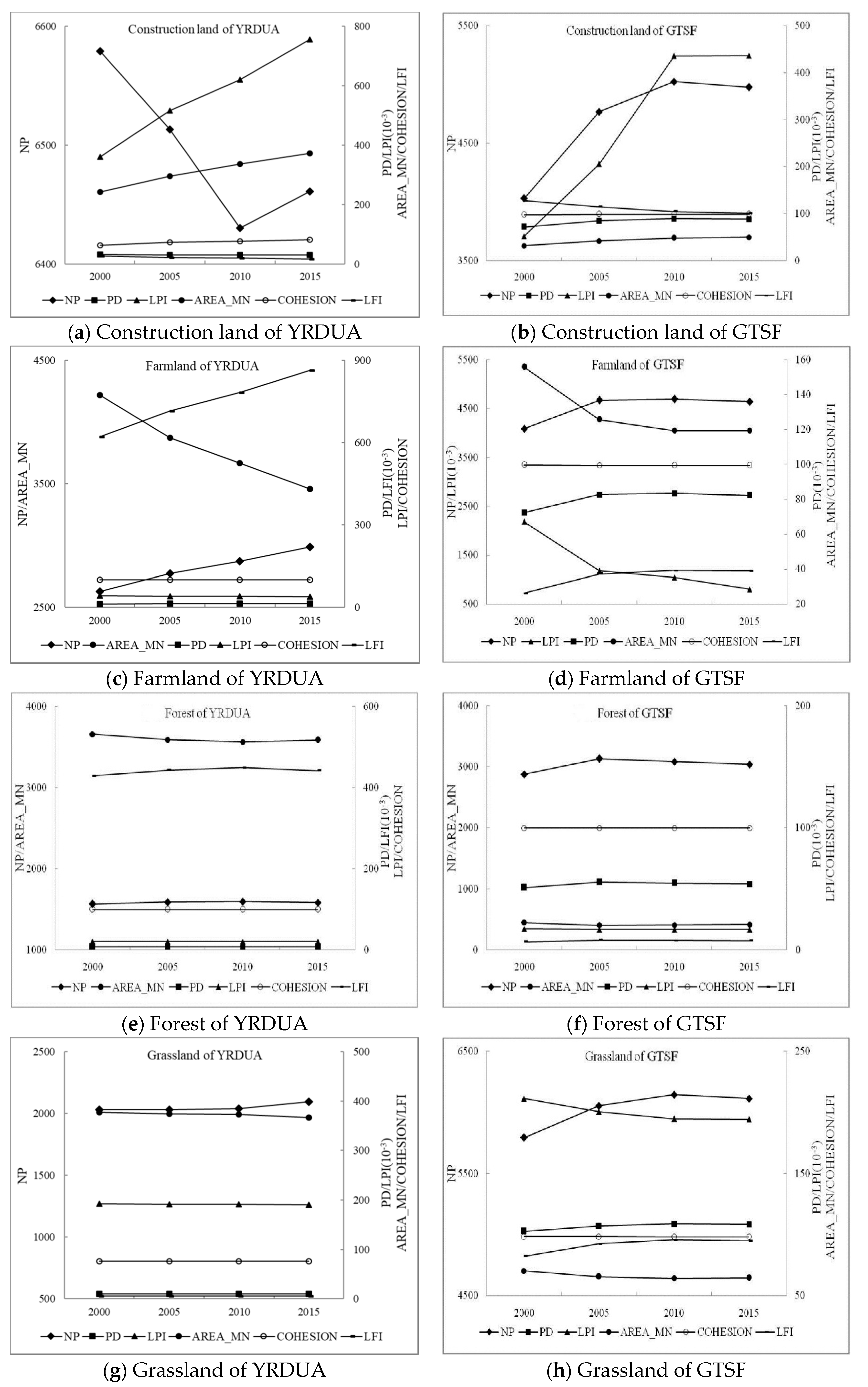
4.3. Changes in Habitat Quality from the Perspective of Landscape Metrics

Here, changes in habitat and non-habitat areas are further discussed from the perspective of landscape patterns. Figure 7a,b plots the values of certain class-level landscape metrics associated with construction land over time in the YRDUA and GTSF. Therein, the values of Mean Patch Area (AREA_MN), Largest Patch Index (LPI), and COHESION grew between 2000 and 2015, while the value of the Landscape Fragmentation Index (LFI) decreased during the same period. This is consistent with the results of previous analyses in which it was found that non-habitat land use became increasingly aggregated over the study period.

Figure 7c–h shows the changes in farmland, forest, and grassland over time across the two sites. In the YRDUA and GTSF, farmland and forest exhibited the largest LPI, respectively, and thus represent the dominant type in the respective case-study area. As already noted, the overall habitat quality in the YRDUA is clearly inferior to that of the GTSF; put differently, the habitat quality of farmland is lower than that of forest.

The different habitats in the GTSF exhibit similar trends in terms of landscape metrics, and there was no further fragmentation of forest after 2005 or of farmland after 2010. In the YRDUA, forest is the second most common landscape type, and the PD and LFI of forest in this area did not increase after 2010, meaning that the degree of fragmentation of this habitat began to decrease gradually after this year, thus leading to improvements in habitat quality.

The values of the COHESION metric were found to slightly decrease over time for most habitats in the GTSF (although the values are large, at ca. 98–100; even the non-habitat COHESION was around 98). In the YRDUA, the values of this landscape metric for farmland and forest were also large, close to 100. Thus, habitats in the YRDUA and habitats and non-habitats in the GTSF were relatively aggregated, including the non-habitat of the GTSF. The COHESION value for construction land in the YRDUA rose from 62.3 in 2000 to 80.8 by 2015; thus, significant aggregation occurred over time but to a lesser extent. In summary, the aggregation of non-habitat areas is higher in the GTSF than in the YRDUA, and therefore the boundary of habitat degradation is clearer in the former, which has higher-quality habitat overall compared to the latter.

As shown in

Table 8. Aggregated changes in class-level landscape metrics over time.

	Year	NP	PD	Area_Mn	CONTAG	Division	LFI
GTSF	2000	17892	0.3171	139.7858	60.0154	0.9700	127.9887
	2005	19848	0.3518	125.2444	58.6348	0.9718	158.4662
	2010	20114	0.3565	124.4887	57.4540	0.9721	161.5649
	2015	19916	0.3530	125.6410	57.3507	0.9721	158.5072
YRDUA	2000	15534	0.0741	1350.0772	42.1290	0.7738	11.5053
	2005	15738	0.0750	1333.2444	40.5114	0.7842	11.8035
	2010	15790	0.0752	1329.1894	39.5566	0.7940	11.8787
	2015	16034	0.0762	1311.7687	38.5584	0.8016	12.2224

, at the overall landscape level, there are certain differences between the landscape metrics in the two urban agglomerations. In the YRDUA from 2000 to 2015, excepting AREA_MN and Contagion (CONTAG), all other metrics exhibited an upward trend. In the GTSF, the NP, PD, and LFI metrics increased from 2000 to 2010 and then decreased from 2010 to 2015, while the opposite was observed for AREA_MN. The remaining two metrics exhibited small increases between 2000 and 2015. The degree of landscape fragmentation was slightly enhanced, and therefore habitat degradation continued.

The degree of fragmentation and the dominant landscape play important roles vis-a-vis habitat quality [49]. In this study, habitat quality was shown to be greatly affected by the fragmentation of habitats and non-habitats, especially in the dominant types. The higher the degree of concentration, the better the habitat quality. Urban agglomeration gradually decreased the fragmentation of construction land, which concomitantly decreased the fragmentation of other habitats, thus leading to gradual improvements in the overall habitat quality. There are several central cities and sub-central cities in the YRDUA that represent concentrations of non-habitat areas and which affect the connectivity of the whole landscape and overall habitat quality.

4.4. Macroeconomic Drivers

Although the YRDUA has become the largest urban agglomeration in China, it developed from a small city cluster. By 1992, it consisted of 14 cities. Then, by 2010, the YRDUA included two cities in Anhui for the first time. The YRDUA maintained an average regional GDP growth rate of over 110% during the periods 2000–2005 and 2005–2010; after 2010, the rate dropped by nearly half, to 63.06%. In terms of the GTSF, the establishment of the Western Taiwan Straits Economic Zone in 2004 enabled the Xiamen special economic zone to play a central role in the region’s economic development. Xiamen City is the geographical, financial, and tourism center of the GTSF, and together with Zhangzhou and Quanzhou, development proceeded in a planned and coordinated way to prevent urban sprawl after 2005. The economy of the GTSF has been developing rapidly; the growth rates of regional GDP in 2000, 2005, and 2010 were 84.95%, 113.25%, and 75.33%, respectively.

As can be seen from

Table 9. Changes in the industrial composition of regional GDP over time for the YRDUA and GTSF.

Year	YRDUA			GTSF
	Primary Industry	Secondary Industry	Tertiary Industry	Primary Industry	Secondary Industry	Tertiary Industry
2000	8.65%	50.41%	40.94%	12.02%	50.05%	37.92%
2005	5.44%	53.46%	41.10%	8.15%	53.20%	38.65%
2010	4.21%	51.30%	44.50%	5.81%	54.16%	40.03%
2015	3.64%	44.77%	51.59%	4.63%	52.82%	42.55%

, between 2000 and 2015, there were clear changes in terms of the contribution of different industry types to the regional GDP in the two urban agglomerations. The proportional contribution of primary (tertiary) industry to GDP has decreased (increased) over time in the YRDUA and GTSF. However, changes in secondary industry over time are more equivocal. The rise of tertiary industry and the fall of primary industry represents a critical change in China’s industrial structure over time. Economic development and an increasing population also correspondingly increase the demand for infrastructure, industry, and residential land. These demands were largely met by displacing farmland and forest, which increased the threats to habitats in these areas.

5. Discussion

From 2000 to 2015, the main trends of land-use changes in the two studied urban agglomerations were (1) the substantial and rapid expansion of construction land and (2) the rapid decrease of farmland and forest resources. There were two distinct transformation periods in both of the urban agglomerations: From 2000 to 2010, the main type of transfer was from other land to construction land, while from 2010 to 2015, the main type was from other land to farmland or forest. Driven by population growth, economic development, agricultural production conditions, and other factors [50], the expansion of construction land encroached on part of the farmland, forest, and grassland. On the other hand, there is a certain rigid demand for construction land to support development; the YRDUA and the GTSF both maintained an average regional GDP growth rate of over 90% between 2000 and 2015, and a corresponding amount of construction land was needed to support such rapid growth. On the other hand, the residents in urban fringe areas and some suburban farmers are also inclined to convert farmland into construction land in order to obtain higher economic benefits [51].

The abovementioned land-use change processes led to the decrease of landscape heterogeneity and the increase of fragmentation. In general, between 2000 and 2015, the overall habitat quality of the eastern, northern, and coastal areas of the YRDUA and the GTSF was relatively low, while that of the southern and western areas was relatively high. A possible reason for the above characteristics is that the eastern coastal areas are mostly plain areas, and frequent human activities interfered strongly with the habitat there, which affected the habitat quality. Meanwhile, the western areas are mostly mountains and hills, and the various biotopes formed by the terrain provide a basis for rich biodiversity [52], forming a benign ecological effect of land use. Additionally, due to the impact of ecological policies such as the return of farmland to forest and grassland, between 2010 and 2015, the forest and grassland in some areas increased and the habitat quality also improved accordingly [20].

Bai et al. [53] stated that forest ecosystems play an important role in water conservation, environmental purification, carbon fixing, and oxygen release. Additionally, Zheng et al. [54] confirmed that land-use change directly caused changes in ecological service value. These findings, together with the results of the present study, suggest that the landscape patterns of forest, farmland, and construction land should be optimized in land-use planning and ecological protection. While maintaining reasonable economic growth, ecological land should be allocated in the process of urbanization. Furthermore, more attention should be paid to the spatial form of urban development in the process of urbanization. The expansion of scattered construction land with low density and low efficiency should be avoided, and the comprehensive renovation of rural idle homesteads and other low-efficiency land should be strengthened so as to reduce the randomness and volatility of the impact of this land on the habitat and improve the connectivity of ecological land and the stability of ecosystems.

However, this study has some deficiencies. For example, due to the lack of quantitative and direct monitoring indicators of regional large-scale habitat quality by remote sensing, at present only indirect assessment of habitat quality based on threats can be carried out. In further work, other sub-modules of the InVEST model could be considered to simulate changes in ecosystem services caused by regional land-use change in order to improve the comprehensiveness of ecological effect assessment.

6. Conclusions

In this study, the spatiotemporal variability of habitat quality was explored in the YRDUA and GTSF by combining the concepts of land use, landscape, and habitat. It was shown that degradation boundaries and improvements in habitat quality from 2000 to 2015 were related to landform, the dominant landscape, and the concentration of non-habitat areas. As a result of the locational advantages offered by coastal areas, the economies of the two urban agglomerations developed rapidly after the launch of the Reform and Opening-up policy in 1978. Urbanization in China is currently characterized by urban agglomerations around core cities. Overall, the results obtained and reviewed herein could prove useful for policymakers and other relevant decision-makers to help ensure that future development in the YRDUA and GTSF proceeds in a manner that optimizes both socioeconomic and environmental objectives simultaneously. As the GTSF is a developing urban agglomeration, the central parts of Xiamen, Zhangzhou, and Quanzhou have become areas with a high concentration of non-habitat, and it is therefore important to optimize the spatial pattern of the dominant landscape and the direction of non-habitat expansion in the GTSF.

References

1. United Nations, Department of Economic and Social Affairs, Population Division. World Urbanization Prospects; United Nations: New York, NY, USA, 2018. [Google Scholar]
2. United Nations Human Settlements Programme. Planning Sustainable Cities; UN-Habitat: Nairobi, Kenya, 2009. [Google Scholar]
3. Tan, Z.-B. Urban Planning; Tsinghua University Press: Beijing, China, 2005. [Google Scholar]
4. Huang, J.; Lin, T.; Zhang, G.-B.; Li, X.-H. Comparative Analysis of the Urbanization Dynamic Characteristics of the Three Major Urban Agglomerations in China. China Popul. Resour. Environ. 2014, 24, 37–44. [Google Scholar] [CrossRef]
5. Gottmann, J. Megalopolis or the urbanization of the northeastern Seaboard. J. Econ. Geogr. 1957, 33, 189–220. [Google Scholar] [CrossRef]
6. Ouyang, Z.-Y.; Zheng, H. Ecological mechanisms of ecosystem services. Acta Ecol. Sin. 2009, 29, 6183–6188. [Google Scholar]
7. Kremen, C.; Williams, N.M.; Aizen, M.A.; Gemmill-Herren, B.; LeBuhn, G.; Minckley, R.; Packer, L.; Potts, S.G.; Roulston, T.; Steffan-Dewenter, I.; et al. Pollination and other ecosystem services produced by mobile organisms: A conceptual framework for the effects of land-use change. Ecol. Lett. 2007, 10, 299–314. [Google Scholar] [CrossRef] [PubMed]
8. Tscharntke, T.; Klein, A.M.; Kruess, A.; Steffan-Dewenter, I.; Thies, C. Landscape perspectives on agricultural intensification and biodiversity-ecosystem service management. Ecol. Lett. 2005, 8, 857–874. [Google Scholar] [CrossRef]
9. Quétier, F.; Lavorel, S.; Thuiller, W.; Davies, I. Plant-trait-based modeling assessment of ecosystem-service sensitivity to land-use change. Ecol. Appl. 2007, 17, 2377–2386. [Google Scholar]
10. Díaz, S.; Lavorel, S.; de Bello, F.; Quétier, F.; Grigulis, K.; Robson, T.M. Incorporating plant functional diversity effects in ecosystem service assessment. Proc. Natl. Acad. Sci. USA 2007, 104, 20684–20689. [Google Scholar] [CrossRef] [Green Version]
11. Ding, Y.-K.; Shan, B.-Q.; Zhao, Y. Assessment of River Habitat Quality in the Hai River Basin, Northern China. Int. J. Environ. Res. Public Health 2015, 12, 11699–11717. [Google Scholar] [CrossRef] [Green Version]
12. Le Maitre, D.-C.; Milton, S.-J.; Jarmain, C.; Colvin, C.-A.; Saayman, I.; Vlok, J.-H.-J. Linking ecosystem services and water resources: Landscape-scale hydrology of the Little Karoo. Front. Ecol. Environ. 2007, 5, 261–270. [Google Scholar] [CrossRef]
13. Tallis, H.T.; Ricketts, T.; Nelson, E.; Ennaanay, D.; Wolny, S.; Olwero, N.; Vigerstol, K.; Pennington, D.; Mendoza, G.; Aukema, J.; et al. InVEST 1.004 Beta User’s Guide. The Natural Capital Project; Stanford University: Stanford, CA, USA, 2010. [Google Scholar]
14. Nelson, E.; Mendoza, G.; Regetz, J.; Polasky, S.; Tallis, H.; Cameron, D.R.; Chan, K.M.A.; Daily, G.C.; Goldstein, J.; Kareiva, P.M.; et al. Modeling multiple ecosystem services, biodiversity conservation, commodity production, and tradeoffs at landscape scales. Front. Ecol. Environ. 2009, 7, 4–11. [Google Scholar] [CrossRef]
15. Li, R. Research on the ecological benefits of soil conservation of Yulin City based on InVEST model. Arid. Zone Res. 2015, 32, 882–889. [Google Scholar]
16. Chen, S.-S.; Liu, K.; Li, T.; Yuan, J.-G. Evaluation of ecological service function of soil conservation in Shangluo City based on InVEST model. Acta Pedol. 2016, 53, 800–807. [Google Scholar]
17. Huang, C.-H.; Yang, J.; Zhang, W.-J. The application of forest inventory data in an ecosystem service evaluation model: InVEST. For. Resour. Manag. 2014, 5, 126–131. [Google Scholar]
18. He, T.; Sun, Y.-J. Dynamic monitoring of forest carbon stocks based on the InVEST model. J. Zhejiang AF Univ. 2016, 33, 377–383. [Google Scholar]
19. Chen, Y.; Qiao, F.; Jiang, L. Effects of land use pattern change on regional scale habitat quality based on InVEST model—A case study in Beijing. Acta Sci. Nat. Univ. Pekin. 2016, 52, 553–562. [Google Scholar]
20. Liu, Z.-F.; Tang, L.-N.; Qiu, Q.-Y.; Xiao, L.-S.; Xu, T.; Yang, L. Temporal and spatial changes in habitat quality based on land-use change in Fujian Province. Acta Ecol. Sin. 2017, 37, 4538–4548. [Google Scholar]
21. Braat, L.; Brink, P.T. The Cost of Policy Inaction (COPI). The Case of not Meeting the 2010 Biodiversity Target; IEEP: The Enveco Meeting, Brussels, Belgium, 2008 17 June. [Google Scholar]
22. Mansoor, D.L.; Marty, D.M.; Eric, C.C.; Lanier, L.N. Quantifying and mapping multiple ecosystem services change in West Africa. Agric. Ecosyst. Environ. 2013, 165, 6–18. [Google Scholar]
23. Stephen, P.; Erik, N.; Derric, P.; Kris, A.J. The Impact of Land-Use Change on Ecosystem Services, Biodiversity and Returns to Landowners: A Case Study in the State of Minnesota. Environ. Resour. Econ. 2011, 48, 219–242. [Google Scholar]
24. Han, J.-R. The Impact of Urban Sprawl on Carbon Stocks Based on the InVEST Model. Master’s Thesis, Northeast Normal University, Jilin, China, 2013. [Google Scholar]
25. He, C.; Zhang, D.; Huang, Q.; Zhao, Y. Assessing the potential impacts of urban expansion on regional carbon storage by linking the LUSD-urban and InVEST models. Environ. Model. Softw. 2016, 75, 44–58. [Google Scholar] [CrossRef]
26. Jiang, W.; Deng, Y.; Tang, Z.; Lei, X.; Chen, Z. Modelling the potential impacts of urban ecosystem changes on carbon storage under different scenarios by linking the CLUE-S and the InVEST models. Ecol. Model. 2017, 345, 30–40. [Google Scholar] [CrossRef]
27. Wang, M.; Ruan, J.-J.; Yao, J.; Sha, C.-Y.; Wang, Q. Study on soil conservation service of ecosystem based on InVEST model-A case study of Ningde City, Fujian Province. Res. Soil. Water. Conserv. 2014, 21, 184–189. [Google Scholar]
28. Wu, J.-S.; Cao, Q.-W.; Shi, S.-Q.; Huang, X.-L.; Lu, Z.-Q. Spatio-temporal variability of habitat quality in Beijing-Tianjin-Hebei Area based on land use change. Chin. J. Appl. Ecol. 2015, 26, 3457–3466. [Google Scholar]
29. Sang, Y.-F.; Wang, Z.-G.; Li, Z.-L.; Liu, C.-M.; Liu, X.-J. Investigation into the daily precipitation variability in the Yangtze River Delta, China. Hydrol. Process. 2013, 27, 175–185. [Google Scholar] [CrossRef]
30. Jiang, W.-H.; Hu, Y.-L. The World’s Sixth Mega-City Group: The Rising of the Yangtze River Delta City Group; Shanghai Academy of Social Sciences Press: Shanghai, China, 2010. [Google Scholar]
31. Liu, G.-L.; Zhang, L.-C.; Zhang, Q. Spaial and temporal dynamics of land use and its influence on ecosystem service value in Yangtze River Delta. Acta Ecol. Sin. 2014, 34, 3311–3319. [Google Scholar]
32. Liu, X.; Ding, Z.-C.; Yang, Y.-X. Strategies Towards a Metropolitan Area with Strong MICE Industry in Minnan Golden Triangle. J. Xiamen Univ. Technol. 2016, 24, 34–40. [Google Scholar]
33. Zhu, L.-C.; Wang, H.-W.; Tang, L.-N. Importance evaluation and spatial distribution analysis of ecosystem services in Min triangle are. Acta Ecol. Sin. 2018, 38, 7254–7268. [Google Scholar]
34. Hall, L.S.; Krausman, P.R.; Morrison, M.L. The habitat concept and a plea for standard terminology. Wildl. Soc. Bull. 1997, 25, 173–182. [Google Scholar]
35. Nelleman, C.; Kullered, L.; Vistnes, I.; Forbes, B.; Foresman, T.; Husby, E.; Kofinas, G.; Kaltenborn, B.; Rouaud, J.; Magomedova, M.; et al. GLOBIO, Global Methodology for Mapping Human Impacts on the Biosphere: The Arctic 2050 Scenario and Global Application; United Nations Environment Programme: Nairobi, Kenya, 2001. [Google Scholar]
36. Mckinney, M.L. Urbanization, biodiversity, and conservation. BioScience 2002, 52, 883–890. [Google Scholar] [CrossRef]
37. Forman, R. Road Ecology: Science and Solutions; Island Press: New York, NY, USA, 2003. [Google Scholar]
38. Bao, Y.-B.; Liu, K.; Li, T.; Hu, S. Effects of Land Use Change on Habitat Based on InVEST Model-Taking Yellow River Wetland Nature Reserve in Shaanxi Province as an Example. Arid. Zone Res. 2015, 32, 622–629. [Google Scholar]
39. Wang, L.-Y. Scenario Simulation for Urban Land Growth Under the Constraint of Ecological Space Quality-A Case of Modified SLEUTH Model. Master’s Thesis, Nanjing University, Nanjing, China, 2016. [Google Scholar]
40. Zhong, L.-N.; Wang, J. Evaluation on effect of land consolidation on habitat quality based on InVEST model. Trans. Chin. Soc. Agric. Eng. 2017, 33, 250–255. [Google Scholar]
41. Rong, Y.-J.; Zhang, H.; Wang, Y.-S. Assessment on Land Use and Biodiversity in Nanjing City Based on Logistic-CA-Markov and InVEST Model. Res. Soil Water. Conserv. 2016, 23, 82–89. [Google Scholar]
42. Wu, J.-Q. Integrated Assessment of Ecosystem in Hainan Bamen Bay Based on CA-Markov and InVEST Models. Master’s Thesis, Hainan University, Hainan, China, 2012. [Google Scholar]
43. Pan, J.-H.; Su, Y.-C.; Huang, Y.-S.; Liu, X. Land use & landscape pattern change and its driving forces in Yumen City. Geogr. Res. 2012, 31, 1631–1639. [Google Scholar]
44. Zhang, M.; Zhu, H.-Y.; He, S.-J. Landscape dynamics of medium- and small-sized cities in eastern and western China: A comparative study of pattern and driving forces. Acta Ecol. Sin. 2013, 33, 275–285. [Google Scholar]
45. Hepcan, S. Analyzing the pattern and connectivity of urban green spaces: A case study of Izmir, Turkey. Urban Ecosyst. 2013, 16, 279–293. [Google Scholar] [CrossRef]
46. Hu, D.-X.; Tang, L.-N.; Qiu, Q.-Y.; Shi, L.-Y.; Shao, G.-F. Decadal temporal changes in landscapes and their driving forces for West-bank Economic Zone of Taiwan Straits. Acta Ecol. Sin. 2015, 35, 6138–6147. [Google Scholar]
47. Jin, T.; An, Y.-L.; Su, X.-L.; Wu, Q.-X.; Zhang, C.; Duan, S.-Q. Research on the Topographic Differentiation of Land Use and Land Use Change in Qingshuijiang Watershed. Ecol. Econ. 2015, 31, 120–125. [Google Scholar]
48. Mao, J.-X.; Li, Z.-G.; Yan, X.-P.; Zhou, S.-H. Research on the Spatio-Temporal Changes of Land Use in Relation to Topography Factors in Shenzhen City. Geogr. Geo-Inf. Sci. 2008, 24, 71–76. [Google Scholar]
49. Liu, S.-L.; Yin, Y.-J.; Yang, Y.-J.; An, N.-N.; Wang, C.; Dong, S.-K. Assessment of the influences of landscape fragmentation on regional habitat quality in the Manwan Basin. Acta Ecol. Sin. 2017, 37, 619–627. [Google Scholar]
50. Hu, Q.-L.; Qi, Y.-Q.; Hu, Y.-C.; Zhang, Y.-C.; Wu, C.-B.; Zhang, G.-L.; Shen, Y.-J. Changes and driving forces of land use/cover and landscape patterns in Beijng-Tianjin-Hebei region. Chin. J. Eco-Agric. 2011, 19, 1182–1189. [Google Scholar] [CrossRef]
51. Wang, X.-J.; Gu, S.-Z.; Dong, D.-K.; Zhang, X.-H.; Wu, H.; Zhou, H. Study on Economic Rationality of Cultivated Land Protection in Typical Case Areas of Shandong Province. China Popul. Resour. Environ. 2011, 21, 61–65. [Google Scholar]
52. Xu, P.; Wang, Y.-K.; Yang, J.-F.; Peng, Y. Identification of hotspots for biodiversity conservation in the Wenchuan earthquake-hit area. Acta Ecol. Sin. 2013, 33, 718–725. [Google Scholar]
53. Bai, Y.; Ouyang, Z.-Y.; Zheng, H.; Xu, W.-H.; Jiang, B.; Fang, Y. Evaluation of the forest ecosystem services in Haihe River Basin, China. Acta Ecol. Sin. 2011, 31, 2029–2039. [Google Scholar]
54. Zheng, J.-K.; Yu, X.-X.; Jia, G.-D.; Xia, B. Dynamic evolution of the ecological services value based on LUCC in Miyun Reservoir Catchment. Trans. CSAE 2010, 26, 315–320. [Google Scholar]
Figure 1. The Yangtze River Delta Urban Agglomeration (YTDUA) and Golden Triangle of Southern Fujian (GTSF).
Sustainability 12 04346 g001
Figure 2. The framework of the methodological process.
Sustainability 12 04346 g002
Figure 3. Spatiotemporal distribution of habitat degradation in the Yangtze River Delta.
Sustainability 12 04346 g003
Figure 4. Spatiotemporal distribution of habitat degradation in the Golden Triangle of Southern Fujian.
Sustainability 12 04346 g004
Figure 5. Spatiotemporal distribution of habitat quality in the Yangtze River Delta.
Sustainability 12 04346 g005
Figure 6. Spatiotemporal distribution of habitat quality in the Golden Triangle of Southern Fujian.
Sustainability 12 04346 g006
Figure 7. Disaggregated changes in class-level landscape metrics over time.
Sustainability 12 04346 g007