Article

Evaluating Dominant Land Use/Land Cover Changes and Predicting Future Scenario in a Rural Region Using a Memoryless Stochastic Method

Centre for Geographical Studies, Institute of Geography and Spatial Planning, Universidade de Lisboa, Rua Branca Edmée Marques, 1600-276 Lisboa, Portugal
*
Author to whom correspondence should be addressed.
Sustainability 2020, 12(10), 4332; https://doi.org/10.3390/su12104332
Submission received: 30 April 2020 / Revised: 22 May 2020 / Accepted: 22 May 2020 / Published: 25 May 2020

Abstract

:
The present study used the official Portuguese land use/land cover (LULC) maps (Carta de Uso e Ocupação do Solo, COS) from 1995, 2007, 2010, 2015, and 2018 to quantify, visualize, and predict the spatiotemporal LULC transitions in the Beja district, a rural region in the southeast of Portugal, which is experiencing marked landscape changes. Here, we computed the conventional transition matrices for in-depth statistical analysis of the LULC changes that have occurred from 1995 to 2018, providing supplementary statistics regarding the vulnerability of inter-class transitions by focusing on the dominant signals of change. We also investigated how the LULC is going to move in the future (2040) based on matrices of current states using the Discrete-Time Markov Chain (DTMC) model. The results revealed that, between 1995 and 2018, about 28% of the Beja district landscape changed. Particularly, croplands remain the predominant LULC class in more than half of the Beja district (in 2018 about 64%). However, the behavior of the inter-class transitions was significantly different between periods, and explicitly revealed that arable land, pastures, and forest were the most dynamic LULC classes. Few dominant (systematic) signals of change during the 1995–2018 period were observed, highlighting the transition of arable land to permanent crops (5%) and to pastures (2.9%), and the transition of pastures to forest (3.5%) and to arable land (2.7%). Simulation results showed that about 25% of the territory is predicted to experience major LULC changes from arable land (−3.81%), permanent crops (+2.93%), and forests (+2.60%) by 2040.

1. Introduction

In many areas of the globe, the scale and extent of land use/land cover (LULC) changes have been affected by socioeconomic and biophysical factors (e.g., [1,2]). More specifically, environmental conditions, internal and external policies, the functioning of local and national markets, and the demographic situation have been pointed out as the main causes directly responsible for the LULC changes [3,4,5]. Therefore, over the last decade, for dynamic visualization and quantification of the spatial patterns of the LULC changes, Geographic Information Systems (GIS) have been widely used, since they allow for the use of vector or remote sensing data, expressed spatially and temporally [6,7,8]. Particularly, LULC change monitoring and assessment is a practice that assists a more conscious and thrifty management of this natural resource, which could result in effective environmental planning and informed policy decisions.
Commonly, in LULC change analysis, the LULC transitions are quantified and visualized based on a transition matrix by computing the inter-class percentage and by measuring, e.g., the persistence, gain/loss, net, and rate of the changes, in order to achieve comprehensive monitoring of physical changes over time [9,10]. Although these are the most commonly used measures, since they are very instructive for understanding the nuance of LULC changes, there are other measures that are equally informative and can contribute to more insights regarding LULC change processes [11] and to the design of anticipatory measure responses to changes. For instance, the quantification of both net change and swap (which comprises both the gain and loss of an LULC class in different locations of the study area), as well the gross gains/losses, allows for the detection of the inter-class transitions that have occurred as a systematic or as a random process of change [11,12]. Thus, the dominant signals of LULC changes can be distinguished.
Hence, whereas a systematic transition occurs by a continuous or general process of change, having a gradual tendency for progressive increment influenced by different factors (e.g., population growth or internal and external policies) [13], a random transition occurs as a single abrupt episode process of change influenced by factors that occur suddenly (e.g., floods or wildfires) [12,13]. Accordingly, distinguishing systematic (dominant) processes within a pattern of LULC changes, which tends to evolve in a progressive way driven by established and continued processes (see, e.g., [12,14]), allows one to focus on the mechanisms of change and further in-depth assessment of the potential change’s main drivers. Therefore, a better understanding of the LULC dynamics and better policies and measures in line can reduce the adverse impacts of dominant LULC changes [12,14,15].
In addition, apart from LULC change dynamics analysis, since the end of the 20th century, the prediction of future scenarios at different spatial and temporal scales has been extensively carried out [16,17,18]. In fact, the study of past and future LULC changes has been very promising for understanding past trends [2] and potential future developments, being a decision-making basis for environmental management and the sustainability of the ecosystems. Therefore, as a complex process, LULC dynamics is regularly modeled through several methods that are efficient in the simulation and prediction of future LULC [19], including the discrete-time Markov chain (DTMC) model (more commonly known as the Markov chain [20]) [21,22], the cellular automata (CA) model [18,23,24], and neural networks [25], among others. Of these approaches, the DTMC model is of countless importance for modeling LULC changes [26,27,28], as it has the advantages of a time dimension and is able to represent the LULC change data, since it has the ability to quantify not only the states of conversion between LULC classes but also the rate of conversion among them. Thus, it is a stochastic process, where space is discrete (i.e., mainly based on probabilities, not certainties).

Context and Background

The last decades of the 20th century and the first decades of the 21st century have shown that European and Mediterranean rural areas have been undergoing significant changes [29,30]. Indeed, one of the most remarkable changes in LULC in Europe, identified in Fuchs et al.’s [2] research, is the increase in forest to the detriment of the agricultural land. Likewise, the same trend has been observed in Portugal [30]. Indeed, the LULC changes in Portugal have been the most dynamic among the European Union (EU) countries [30,31].
For instance, despite the existence of numerous studies regarding the LULC changes in Portugal [32,33,34], the primary research focus has been on urban areas rather than rural areas. However, rural areas and agriculture have an important role in the regional and national economy of individual countries, as they constitute an important source of income for part of the population. Therefore, it is urgent to monitor the dynamics of rural LULC changes to promote and ensure a weighted and parsimonious use of the available resources.
Accordingly, given the stark changes of the Portuguese landscape, this study seeks to unravel the LULC changes situation in the Beja district, the largest Portuguese district in terms of area and the second in terms of percentage of agricultural land (about 47% in 2010); a rural region where we can find the Montado (named Montado in Portugal and Dehesa in Spain), an agrosilvopastoral agricultural heritage system [35,36], that has been indicated as a globally important agricultural system according to the Globally Important Agricultural Heritage System (GIAHS) program promoted by the Food and Agriculture Organization of the United Nations (FAO) [37].
Moreover, this research is an effort to evaluate the spatiotemporal LULC changes with a particular focus on the evaluation of the dominant LULC changes and to simulate the future changes, in order to determine the main LULC processes’ transformations and suggest new strategies for formulating better land use policies. The analysis was performed in a 10,229.05 km² area in the southeast of Portugal, which is experiencing marked landscape changes [32]. Thus, the main objectives of the present study were threefold: (i) identify and analyze the spatiotemporal dynamics of LULC over the past 23 years (1995–2018); (ii) quantify and analyze in depth the inter-class dominant (systematic) LULC transitions; and (iii) quantify the states of conversion between LULC classes and simulate and analyze the future LULC changes by 2040 using the DTMC model.
Our research is organized as follows: Section 2 details the study area, the used data, and the applied methodology. The results of the LULC changes and future LULC developments are described in Section 3. Finally, in Section 4, we discussed the main findings of our results and the implications of the applied methodology, presenting also the main conclusions of our research.

2. Materials and Methods

2.1. Study Area

The study area, the Beja district, is located between 07°37′58″ W and 07°41′17″ W longitude and between 38°08′35″ N and 38°10′08″ N latitude in the southeast of Portugal in the Nomenclature of Territorial Units for Statistics (NUTS) II Alentejo litoral and Baixo Alentejo (Figure 1). The district of Beja is bordered to the north by the Évora district, to the south by the Algarve region, to the east by Spain, and to the west by the district of Setúbal and the Atlantic Ocean. Beja is the largest Portuguese district, with an area of 10,229.05 km² and a resident population of 152,758 inhabitants in 2011 [38].
This region is characterized by a vast landscape of wheat, cork oaks, and olive trees, where the dominant land use is mixed agrosilvopastoral. The landscape of this region is distinctive, with both fragmented parcels and more compact parcels of land due to the different cropping calendars and field geometries. Dispersed settlements are the predominant urban form in this region. The climate is influenced by its distance from the coast, with a Mediterranean climate characterized by hot and dry summers and wet and cold winters. To the southeast, the territory is flat; to the north and west, the extensive plains are cut by tiny hills, the valley of the Guadiana River is the district’s main geographical feature, which crosses from north to south in the eastern part of the district. The Alqueva dam, the largest in the country, is located in this district.

2.2. Official Portuguese Land Cover (COS) Data

The official spatial land cover data (COS) produced by the Portuguese General Directorate for Territorial Development (DGT) for 1995, 2007, 2010, 2015, and 2018 were used. These maps have the highest cartographic detail for the study area and are available for free on the DGT website (http://mapas.dgterritorio.pt/geoportal/catalogo.html). The COS maps are produced by photointerpretation (i.e., over orthophoto maps), with vector (polygons) structure data, a cartographic accuracy of 0.5 m, a minimum mapping unit (MMU) of 1 ha, and a scale of 1:25,000 [39]. The five datasets have a hierarchical nomenclature system (a DGT report describes in detail the COS nomenclature characteristics [39]).
Spatiotemporal LULC change analysis was developed considering three major classes of the first hierarchical level of the COS nomenclature, namely, artificial surfaces, forest, and water bodies. In order to specify the major changes in croplands and characterize the type of agricultural activity in this region, we used the second hierarchical level of the COS nomenclature of the agriculture mega class, namely arable land, permanent crops, pastures, and heterogeneous areas. Therefore, a total of seven classes were used (Table 1). All LULC maps were clipped to the extent of the case study area, converted to a raster format of 100 × 100 m, and reclassified into seven classes. The cartographic information treatment and the spatiotemporal analysis were developed in QGIS software.

2.3. Spatiotemporal LULC Change Analysis

To identify and analyze the spatiotemporal dynamics of LULC in the Beja district, we first presented a brief evolution and distribution analysis of each class between 1995 and 2018. We quantified the changes for each year and reported them spatially and temporally. Secondly, we computed four change matrices in order to understand the main transition dynamics within each LULC class during the periods 1995–2007, 2007–2010, 2010–2015, and 2015–2018. The matrices were presented in graphical form. Each graph for each period shows the changes within each class from the initial time to the final time.

2.4. LULC Change Detection

For the LULC change detection in-depth analysis, we compared two maps (1995 and 2018) and produced a cross-tabulation matrix for the overall period (1995–2018). We decided to only analyze the overall period since each period comprises different years. While the first period has 12 years (1995–2007), the second (2007–2010) and the last (2015–2018) have 3 years, and the third has 5 years (2010–2015), so the change detection analysis could be influenced by the year’s discrepancy between periods. Thus, the transition matrix represents the percentage of LULC changes within each class (j), where the diagonal values indicate the percentage of LULC that persists ( P j j ) for each LULC class from initial time ( T 1 ) (1995) to the final time ( T 2 ) (2018), rows indicating the transitions from initial time ( P j + ) , and columns indicating the transitions in the final time   ( P + j ) .
By following Pontius et al.’s [11] study, we obtained several measures from the transition matrix result and grouped them into two categories. The first category includes the (i) persistence, (ii) gain, (iii) loss, (iv) total change, (v) absolute value of net change, and (vi) swapping tendency. Since net change cannot detect the swap between each class, and therefore underestimates the LULC total change, the swapping tendency is calculated, since it comprises both the gain and loss of an LULC class in different locations of the study area [11]. Additionally, we presented the LULC vulnerability to transition by calculating the gain-to-loss, lost-to-persistence, and the gain-to-persistence ratios. A description of each measure is in Table 2.
The second category includes the measurement of systematic and random LULC changes by using the off-diagonal entries of the transition matrix (which indicates the transitions from one LULC class to the other) for the significant inter-class transitions detection. To detect if the inter-class transition is systematic or random, the expected LULC value was compared with the observed LULC value in the matrix. Following the statistical definitions outlined by Pontius et al. [40], a random transition indicates that the gain from other LULC classes was equivalent to the size of those other losing classes, or the loss to other LULC classes was equivalent to the size of those other gaining classes. Therefore, values close to zero or at zero indicate a partly systematic or random transition, respectively, while numbers far from zero indicate a systematic inter-class transition [11].
As such, the measurement of the systematic and random LULC transitions will result in three values in terms of gain ( G i j ) and in three values in terms of loss ( L i j ) . Firstly, we compute the expected LULC gains percentage if the gain in each class were to occur randomly:
G i j = ( P + j P j j ) ( P i + i = 1 ,   i j   j P i + )
where ( P + j P j j ) is the total gross gain of LULC class j, and P i + is the size of LULC class i in the initial time (1995). i = 1 ,   i j   j P i + is the sum of the sizes of all LULC classes, excluding LULC classes of j, in the initial time. Secondly, we compute the expected LULC losses percentage if the loss in each class were to occur randomly:
L i j = ( P i + P i i ) ( P + j j = 1 , j j   j P + j )
where ( P i + P i i ) is the observed total gross loss of LULC class i, and P + j is the size of LULC class j in the final time (2018). j = 1 , j j   j P + j is the sum of the sizes of all LULC classes, excluding LULC classes of j, in the final time.
Third, we compute the differences between the observed LULC percentage and the expected LULC percentage under a random process of gain:
P i j G i j
where P i j is the observed LULC, and G i j   is the expected LULC if the gain in each class were to occur randomly. Fourth, we compute the differences between the observed LULC percentage and the expected LULC percentage under a random process of loss:
P i j L i j
where P i j is the observed LULC, and L i j is the expected LULC if the loss in each class were to occur randomly.

2.5. The Discrete-Time Markov Chain (DTMC) Model

2.5.1. States Transition Probability of the Markov Chain

To quantify the states of conversion between the LULC classes and simulate and analyze the future LULC changes by 2040, we used the Discrete-Time Markov Chain (DTMC) model. Specifically, the DTMC model use matrices to model the LULC transition probabilities among a set of discrete states. Therefore, a DTMC is characterized by an array of random variables X 1 ,   X 2 ,   ,   X n showing a memoryless property (i.e., a Markov property). The memoryless property postulates that the transition probabilities are independent of the chain state before its current state. Thus, the X n + 1 state distribution relies only upon the current state X n regardless of the X n 1 ,   X n 2 ,   ,   X n 1 states.
P r ( X n + 1 = x n + 1 | X 1 = x 1 ,   X 2 = x 2 ,   ,   X n = x n ) = P r ( X n + 1 = x n + 1 | X n = x n )
Strictly, a Markov chain is a probabilistic automaton, where X n has a set of possible states S = { S 1 ,   S 2 ,   ,   S r } entitled as the “state space of the chain.” The procedure begins in one of S states and changes consecutively from one to another. Each change is named either step or transition, and the transition probability p i j is set as the probability of change from state s i to state s j in just one step.
p i j = P r ( X 1 = s j | X 0 = s i )
whereas the probability to change from state s i to state s j in n steps is given by p i j ( n ) = P r ( X n = s j | X 0 = s i ) .
If Equation (7) proves to be true, the DTMC is time-homogeneous, which indicates that the original transition probabilities remain unchanged through time.
P r ( X n + 1 = s j | X n = s i ) = P r ( X n = s j | X n 1 = s i )
For k > 0 , if p i j = P r ( X k + 1 = s j | X k = s i )     p i j ( n ) = P r ( X n + k = s j | X k = s i ) , then the Markov chain is said to be time-homogeneous. The transition probability can be represented as a transition probabilities matrix (or simply transition matrix) P = ( p i j ) i , j , where each element ( i , j ) denotes the position of p i j .
P = [ p i i p i j p j i p j j ]
The dispersion through the states can be transcribed as a stochastic ( i x i = 1 , x i 0 ) row vector x . Hence, x ( 1 ) relates to x ( 0 ) as x ( 1 ) = x ( 0 ) P and, recursively, we have x ( 2 ) = x ( 0 ) P 2     x ( n ) = x ( 0 ) P n .

2.5.2. Classification States and Simulating Future States

The states can be classified by means of their periodicity. A state that is not absorbing is a transient one. A state s i is said to be transient if there is a state s k that is attainable from s j , but j not being attainable from s k . In other words, if s j is transient, there is no guarantee that, after leaving s j , the system will return there. Suppose that, for a chain with initial state x , the number of periods required to return to that state is given by T x x . If P ( T x x < + ) = 1   P ( T x x = + ) > 0 , the x state is transient.
A state s j is said to be recurrent if it is not transient, i.e., if it is always possible to return to s j . As such,
s t a t e   x   i s   r e c u r r e n t   i f P ( T x x < + ) = 1   o r P ( T x x = + ) = 1 i n   a d d i t i o n   i s { n u l l   r e c u r r e n t   i f   P ( T x x ) = + p o s i t i v e   r e c u r r e n t   i f   P ( T x x ) < + a b s o r b i n g   i f   P ( T x x = 1 ) = 1
The time necessary to reach a specific state can also be computed. The so-called hitting time, i.e., the first passage ( s i s j ) , is given by the number of steps ( T i j ) that the chain requires until it hits the state s j for the first time, considering that X 0 = s i .
h i j ( n ) = P r ( T i j = n ) = P r ( X n = s j ,     X n 1 s j ,   ,   X 1 s j | X 0 = s i )
where h i j ( n ) = k S { s j } p i k h k j ( n 1 ) and h i j ( n ) = p i j .
A measure interconnected with ( h ) h that is frequently used is the mean first passage time, i.e., the expected hitting time. In an ergodic Markov chain, the mean first passage time from s i to s j is the estimated number of steps necessary to go from the initial state s i to s j for the first time. This measure is the ( h ) average value, explicitly   h ¯ i j = n = 1 n h i j ( n ) . When delineating the first passage time, one can assume that s i = s i j and thus obtain the first recurrence time T i = i n f { n 1 :   X n = s i | X 0 = s i } .
Therefore, having the recurrent states, we calculated the mean recurrence time, i.e., the expected number of steps to return to the initial state:
r i = k = 1 k P ( T i = k )
Finally, as the period under analysis presents different cycles, that is more dynamic cycles (1995–2007 and 2010–2015) interspersed with less dynamic ones (2007–2010 and 2015–2018), we chose to perform future simulations based on trends of the whole set (1995–2018). Thus, based on the year 2018 and using the trends recorded over 23 years, we created a scenario of LULC for 2040 (instead of 2041 for rounding purposes).

2.5.3. Uncertainty of Future States

Uncertainty can then be characterized by the probability vectors that are produced as a sub-product of simulation, made available by most stochastic modeling procedures [41]. These probabilities provide useful information about the quality of the resulting classification in terms of the uncertainties involved. To fully explore the information of the probability vector, additional measures of uncertainty are needed [42]. The greater the uncertainty, the lower the probability that a pixel will be associated with a given class, so uncertainty is the complement of the probability. Formally, if we considerer P i j , the probability that a given pixel j is associated with class i , the uncertainty can be described by U i j = 1 P i j .
However, normally the true class of the pixel is not known and, consequently, the amount of information required to indicate the pixel class is also unknown. The pixel entropy is therefore defined as the expected information index of a piece of information that reveals your true class. For this purpose, the entropy measure combines the uncertainties of the various pixel classes, weighing them by their probabilities. In this way, the global entropy can be estimated from the normalized values of probabilities by class, using the expression E i j = P i j log P 2 i j .

3. Results

3.1. LULC Spatiotemporal Evolution and Distribution

The spatiotemporal analysis results showed that the Beja district has undergone major changes between 1995 and 2018 (Table 3). At first sight, the predominance of agricultural and forestry areas over the entire study period was observed. However, the occupancy tendency of both classes showed large fluctuations. Examining the results, between 1995 and 2010, there was a loss of almost 6.6% of the agricultural area, but this mega class continued to occupy the largest portion of the territory (in 2010 about 62.88%). Subsequent years (2015–2018) saw an increase in agricultural area (+1.08%).
Indeed, except for the permanent crops, there has been a significant decrease in remaining croplands. Particularly, arable land, the cropland with the most significant predominance in the Beja district (in 2018 about 20.7%), presented a decrease of almost 6% between 1995 and 2018, while heterogeneous areas and pastures decreased by about 2% and 2.6%, respectively. Heterogeneous areas are mainly concentrated near forestland, and the pastures class almost disappears in the central region of the Beja district. Permanent crops increased by about 5%, particularly in the northern part of the district, where the patch correspondent to this class is noticeable (Figure 2).
By contrast, the forestland presented an area increase of almost 5.6% between 1995 and 2010 (in 2010 about 34%), but in subsequent years (2010–2018) there was a loss of almost 1.3% (in 2018 about 32.7%). It is noticeable that the green area corresponds to the forestland class in the SSW of the study area, probably due to its being closer to the Atlantic Ocean and to its orography (plateaus). However, the increase in forest was especially near the wetlands, untangling the southeast part of the district. As for the artificial surfaces, although substantially reduced in this region, they present a linear growth increment between the period under analysis (close to 0.5%), especially in the north of the district near the Beja airport. The same occurred with the wetlands class with an overall increase of 0.7%, with some visible expression in the northeast part of the district (Figure 2).

3.2. Main LULC Transitions by Period

The analysis of the inter-class transitions by period is present using the cross-tabulation matrices in graphical form for the four periods under analysis (Figure 3). Specifically, during the first period (1995–2007), almost 20% of the LULC changed. The results revealed a clear tendency for each type of agricultural use to transition to another agricultural use or to transition to forest. Additionally, the forest class and the pastures class were the two that presented the highest LULC transition values. Indeed, the first period experienced a significant decrease in croplands (−6.3%), mostly due to forestland, with transitions from the pastures (3.8%), heterogeneous areas (1.8%), and arable land (1.7%) classes. However, about 1.8% of forestland also transitioned to agricultural areas. By contrast, arable land and pastures exchange between themselves.
As for the second period (2007–2010), about 3% of the LULC changed. This period experienced the same trend: a decrease in croplands, albeit much less significant (−0.42%). The arable land, pastures, and permanent crops classes transitioned between each other, the highest area transitioning from arable land to permanent crops (0.8%).
The subsequent period (2010–2015) experienced about 8.5% of LULC changes. However, this period counters the decreasing trend in cropland, albeit modestly, as croplands increased but only by about 0.24%. Thus, a transition tendency similar to the first period can be observed, since the major recorded transitions were between agricultural areas and forestland. Accordingly, the heterogeneous areas and forestland classes transitioned between each other, with heterogeneous areas transitioning to forest (1.18%) and forest transitioning to heterogeneous areas (1.55%).
During the last period (2015–2018), almost 4.7% of the LULC changed. This period experienced the highest gain in agricultural areas (+0.84%). Once again, arable land transitioned mainly to pastures (0.7%), and pastures transitioned mainly to arable land (0.5%), while heterogeneous areas transitioned to arable land (0.7%) and to pastures (0.7%). Indeed, the most substantial transition recorded was from arable land to permanent crops (1.8%), followed by the transition from forest to pastures (0.7%), and from arable land to pastures (0.6%). Unlike the past two periods, we verified for the first time more losses than gains for the forest class.

3.3. LULC Change Detection

The in-depth analysis of the overall LULC change detection shows that, for the overall period (1995–2018), about 72.1% of the LULC persisted, while 27.9% exhibited transitions. Briefly, the highest LULC transitions were experienced from arable land to permanent crops (4.96%), followed by the transition from pastures to forest (3.48%) (Table 4). In addition, the overall period transitions highlighted that forest experienced high gains from agricultural classes, while both artificial surfaces and water bodies showed a minor transition to other LULC classes.
From Table 5, it can be verified that, during the overall period, both the artificial surfaces and water bodies classes experienced a lower percentage of persistence (0.76% and 1.36%, respectively). These results are mostly due to their lower percentage of territory occupancy within the period analysis. Thus, artificial surfaces occupied about 1.2% of the district area, meaning almost 0.5% of gains and only 0.03% of losses. Therefore, the changes in the artificial surfaces class is mostly net change (about 0.45%). Similarly, the water bodies class experienced almost 0.8% of gains against 0.1% of losses between 1995 and 2018. Thus, most of the change in the water bodies class is a net change (0.7%). Hence, artificial surfaces and water bodies experienced a gain–loss ratio of 18.3 and 10.5, respectively; however, according to the loss-to-persistence and gain-to-persistence ratios, both classes presented a greater tendency to persist than to gain or lose. Figure 4 presents the net changes for both the artificial surfaces and water bodies classes. While artificial surfaces gains are highly dispersed across the district and usually founded near spots with the same LULC, water bodies gains are not clustered predominantly near to each other. Due to the minimal losses during 1995–2018, it is difficult to identify the dispersion of losses across the district.
In contrast, forest, arable land, and heterogeneous areas presented a high percentage of persistence (24.66%, 16.47%, and 16.23%, respectively), while pastures and permanent crops presented a relatively low percentage of persistence (6.52% and 6.14%, respectively). These results are mostly due to each LULC class percentage of territory occupancy during all the years under study. Nevertheless, permanent crops and forest classes presented more gains than losses during the overall period. The gain–loss ratio indicates that permanent crops presented 4.9 times more gain than loss, while forest presented a ratio of 2.2 times more. However, the influence of net changes was found to be the main driver in permanent crops (66% of the total change for permanent crops), while swapping was the main driver in the forest class (63% of the total change for forest).
However, according to the loss-to-persistence and gain-to-persistence ratios, the forest class experienced a greater tendency to persist than to gain or lose, while the permanent crops class presented a greater tendency to persist than to lose and a greater tendency to gain than to persist. Figure 5 presents the net changes for both the permanent crops and forest classes. The gains of forestland are dispersedly distributed across the Beja district and are usually found near spots with the same LULC. Comparatively, permanent crops gains are primarily distributed in the north and east. Gain spots are grouped mainly near to each other, while losses are minimal and show no distribution pattern.
The remaining agricultural classes presented more losses than gains, with a loss–gain ratio of 2.4, 1.5, and 1.7 for arable land, pastures, and heterogeneous areas, respectively. These three agricultural classes indicate both swap and net changes between 1995 and 2018. However, the influence of swapping was found to be the main driver of the total change, which was a change by 59%, 79%, and 75% for arable land, pastures, and heterogeneous areas, respectively. While both arable land and heterogeneous areas presented a greater tendency to persist than to gain or lose, the pastures class presented a greater tendency to lose than to persist and a greater tendency to persist than to gain.
Figure 6 presents the net changes for arable land, pastures, and heterogeneous areas. The three classes present a very distinct change pattern. Arable land losses are mainly consolidated in the north and east of Beja, while the gains are dispersed in the south of the district, predominantly near spots with the same LULC. As for pastures, the gains are spread over the entire territory, while the losses can be found in the south and close to the east. Lastly, the heterogeneous areas show large gains in the center of the territory, while losses are distributed mainly close to where there is forestland.

3.4. Detection of Random and Systematic LULC Transitions

The random and systematic LULC transitions analysis showed that not all the inter-class transitions during the period under analysis were systematic (dominant) processes within a pattern of LULC changes. Based on Table 6 and Table 7, we are able to determine what the dominant transitions in each LULC class would be if the gain or loss in each class were to occur randomly. Therefore, the arable land and permanent crops classes experienced the strongest dominant signal of change. While arable land systematically transitioned to permanent crops, permanent crops were systematically gaining from arable land simultaneously (3.12%), and arable land was also systematically losing to permanent crops (3.35%). However, permanent crops systematically avoided losses to arable land.
Likewise, while arable land systematically transitioned to pastures, the pastures class was systematically gaining from arable land simultaneously (1.37%), and arable land was also systematically losing to pastures (1.44%). By contrast, while pastures were systematically transitioning to arable land, arable land was systematically gaining from pastures simultaneously (1.88%), and pastures were also systematically losing to arable land (0.92%). Thus, the arable land and pastures classes systematically transitioned between each other. Analyzing the situation more closely, based on Table 6, it should also be noted that permanent crops and arable land systematically avoided gaining from forest (−1.85% and −1.27%, respectively), and permanent crops or arable land avoided gaining from heterogeneous areas (−1.07% and −0.59%, respectively). In Table 7, it can be seen that arable land systematically avoided losing to heterogeneous areas (−2.29%) or to forest (−2.41%), and pastures avoided losing to heterogeneous areas (−1.39%).
Even though forest systematically gained from pastures (1.91%), there was a weak signal of pastures losing to forest (0.68). The analysis of the results in Table 6 also recognized that pastures systematically avoided gaining from forest (−0.89%), while Table 7 indicated that pastures avoided losing to heterogeneous areas (−1.39%). On the one hand, heterogeneous areas systematically gained from forests (1.06%), while heterogeneous areas systematically avoid losing to forest (0.51%). However, forest was systematically losing to heterogeneous areas (1.08%). From Table 6, it also appeared that forest and heterogeneous area classes systematically avoided gaining from arable land (−1.20% and −0.84%, respectively), and forest avoided gaining from permanent crops (−0.66%).

3.5. States Transition Probability of the Markov Chain

Table 8 presents the temporal transition probability matrix for the overall period (1995–2018), showing the probability that each LULC type transitions to another (the off-diagonal entries indicate the transitions probability from one LULC class to another). As expected, there is a small probability that artificial surfaces will transition to another use (3%), and the same is observed with the water bodies (5%). For forest areas, there is a probability of an approximately 13% change in use, specifically, approximately 8% towards heterogeneous areas.
With regard to croplands, there is a clear tendency for each type of agricultural use to transition to another agricultural use or to forest. For example, pastures and arable land are the classes that are most likely to transition. Pastures have a 25% probability of transition to forest and a 19% probability of transition to arable land. Arable land presents a 19% probability of transition to permanent crops and an 11% probability of transition to pastures. Heterogeneous areas have a 12% probability of transition to forest. From all croplands, the low probability of permanent crops to transition (about 17%) and the low probability of heterogeneous areas to transition (about 24%) to other LULC classes are noteworthy.

3.6. Classification States

The analysis in Section 3.5 showed that each state has a positive probability to achieve any other state. Therefore, all states of the DTMC communicate, and the matrix can be cataloged as irreducible. As there are no transition or absorbing states, the matrix is also recurrent; i.e., all states are recurrent. Finally, as we always obtain k = 1 , the recurrent states are all aperiodic. Together, since all states are recurrent and aperiodic, communicating the matrix can be cataloged as ergodic. Thus, having a transition probability matrix, the mean first passage time was evaluated. Table 9 gives us the mean first passage time between 1995 and 2018. It is clear that a high number of steps are expected to be necessary for transition to artificial surfaces and water bodies, suggesting that both of these LULC classes are almost stable. Faster transitions are, in all cases, towards a forest state.
Having the recurrent states, we calculated the mean recurrence time, i.e., the expected number of steps to return to the initial state. This measure is narrowly related to the mean first passage and states. Even in our case, a returning probability of 1 does not signify that the predictable return time is fixed. The results showed that all the LULC classes represent positive recurrent states (Table 10). Thus, if the system initiates in state s i , in determining the number of steps necessary to return to s i for the first time, it is obvious that it will eventually return to the initial sate. This is because, in the first step, the system either stays at s i or changes to other state s j , and from that state s j , one will ultimately reach s i since the chain is ergodic.
From Table 10, it is noticeable that, in the first period (1995–2005), the LULC classes with the lowest mean recurrence time are forest (7.5) and water bodies (1.4), which denotes the resilience of these two LULC classes. The next period (2005–2010) is similar to the previous one, but we start to see the emergence of permanent crops (9.2). The last two periods emphasize the importance of forest and permanent crops in the study area. However, the roles invert themselves, since in 2015–2018, permanent crops achieved a major role in the landscape of Beja, and this may soon become an absorbing state. As for the overall period from 1995 to 2018, we can confirm the forest resilience with a lower value (2.97), whereas the different changing cycles slightly reduce the importance of permanent crops, especially due to the dynamics between 1995 and 2007.
Table 11 shows that, on average, and after some time, following the 2015–2018 trend, 67% of the area will be permanent crops. Likewise, considering the 2010–2015 trend, about 20% of the territory will be arable land and about 25% forestland. In the former periods of 1995–2005 and 2005–2010, it could be expected that 72% and 65% of the Beja district area will be water bodies, respectively. Lastly, the analysis of the overall period (1995–2018) allows us to embrace the different dynamics observed, avoiding trends too ephemeral to be considered in the long term and reconfirming forestland as the most likely class to occur.

3.7. Simulating Future States

As stated before, in our recurrent positive (i.e., having a stationary distribution) and aperiodic matrix, regardless of the initial probabilities, as the time step increases towards infinity, the chain probability distribution converges. In this case, the chain has a limiting distribution, i.e., a stationary distribution. In Figure 7, we inspect a random simulation of p i j ( n ) through time and show that, taking into account the 1995–2015 probability vector (Figure 7a), states converge to two vectors. The probability of being in States 1 (artificial surfaces) and 7 (forest) converges to higher values than the others LULC classes. Over the long term (e.g., after 48 time steps), the increasing probability of becoming forest overcomes the decreasing probability of becoming artificial surfaces.
As for Figure 7b, where we focus on the most recent trend (2015–2018), the situation is somewhat similar. While the system evolves to infinity, the probability vector converges to a vector assigning most of the probability to State 3 (permanent crops). In this case, the probability of becoming permanent crops overpasses that of becoming artificial surfaces only after 28 time steps. In addition, the decreasing rate of the probability of becoming artificial surfaces is much higher in b) than in a). Lastly, it was confirmed that the empirical probabilities behave in the same way (Figure 8).
Therefore, the future state simulation results showed that, in 2040, about 25% of the territory can transition use, and about 21% of that territory corresponds to agricultural land. Accordingly, the major changes concern cropland areas, with a predicted decrease of about −3.67% in 2040 (total 60.3%) (Figure 9). However, this situation hides very different behaviors for each cropland class, since arable land (−3.81%), pastures (−1.35%), and heterogeneous areas (−1.02%) diminish. In contrast, and following the trend of past years, permanent crops will see its importance continue to rise (+2.93%). The remaining LULC classes will continue expanding until 2040, where forest class will increase by about 2.60%, artificial surfaces will increase by about 0.40%, and water bodies will increase by about 0.65%. Figure 9 shows the spatial distribution of LULC by 2040.
In Figure 10a, we have the uncertainty map for the 2040 LULC simulation, with values ranging from 0.03 to 0.53. Crossing these values with LULC classes shows us where the model performs better. Thus, we have two classes that are very resilient and are therefore modeled with a low degree of uncertainty: artificial surfaces and water bodies, both with an average uncertainty of 0.03. Next, also with low values, are the two most dynamic and important classes of the study area, namely, forest (0.13) and permanent crops (0.17). Finally, three classes remain, which, due to their complex structure and overlapping, achieve the worst values: heterogeneous areas (0.23), arable land (0.38), and pastures (0.53). In Figure 10b, we have a spatial notion of the entropy distribution with values oscillating between 0.28 and 1.95. Spatially, both calculations, uncertainty and entropy, show a high rate of agreement.

4. Discussion and Conclusions

In recent decades, the abandonment of agricultural land has been an international trend. In Portugal, this has occurred, confirming marked changes in the agricultural landscape [30,
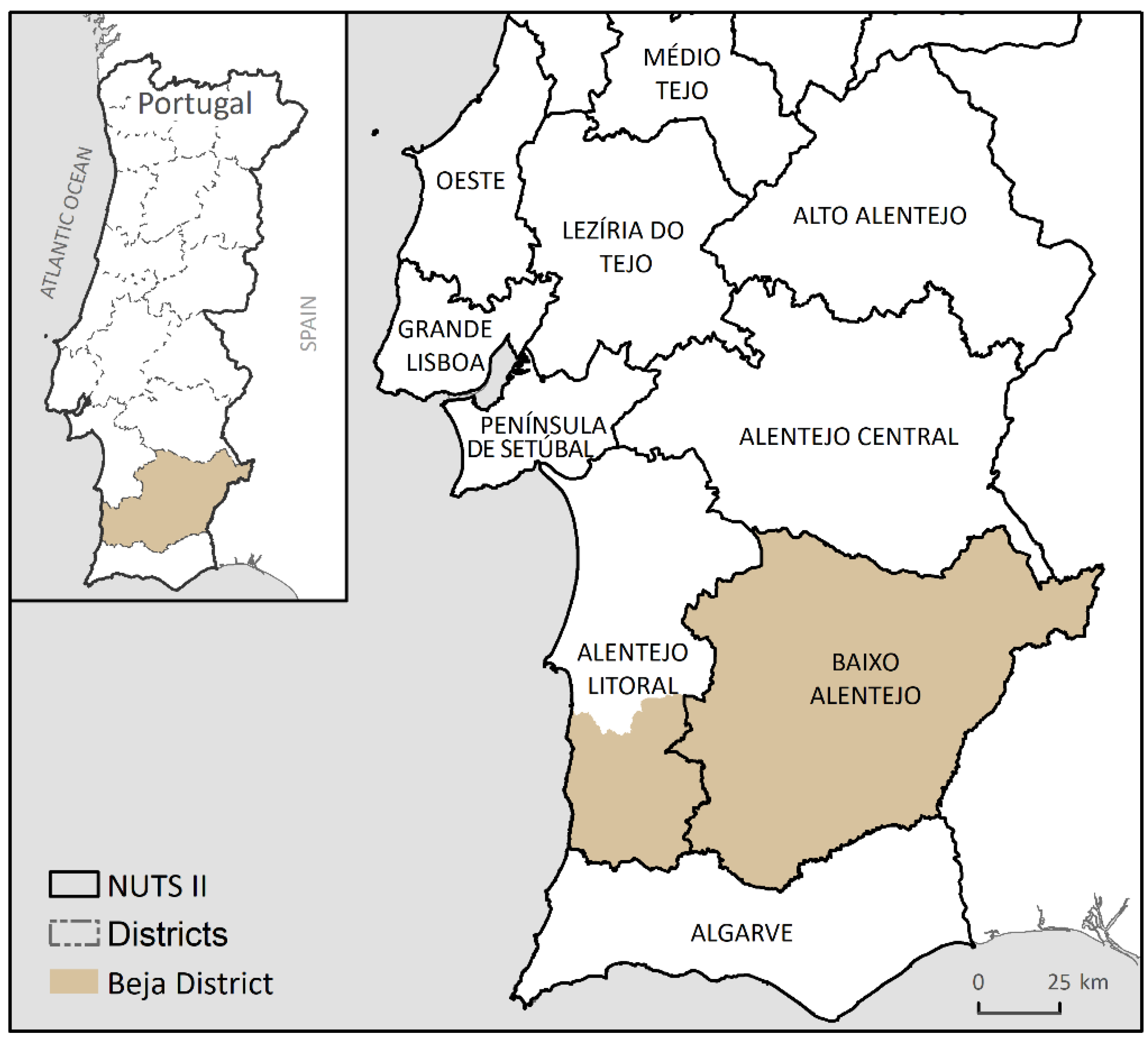
31]. Therefore, in this study, we analyzed the spatiotemporal changes that occurred in the largest district of Portugal, Beja, which has an agricultural economic background, and provided a trend projection for the year of 2040. Accordingly, the monitoring of the dynamics of LULC at the regional level revealed noteworthy LULC dynamics intrinsically associated with distinct agricultural practices of food production and distribution.

4.1. About the LULC Changes Detection

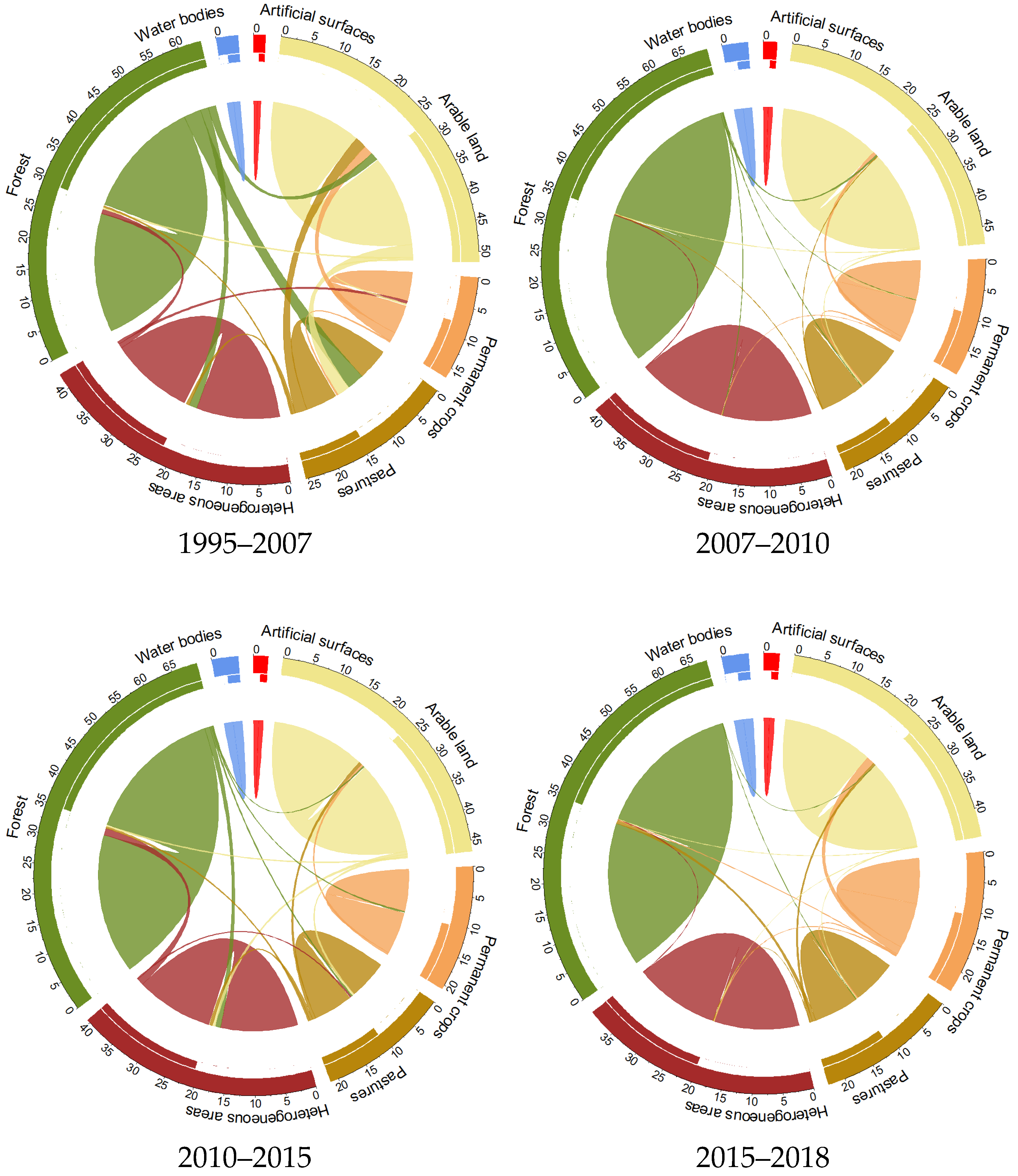
The degree of transition between the LULC classes in the Beja district was significantly different during each period under analysis. The following findings are worth noting:
(i)
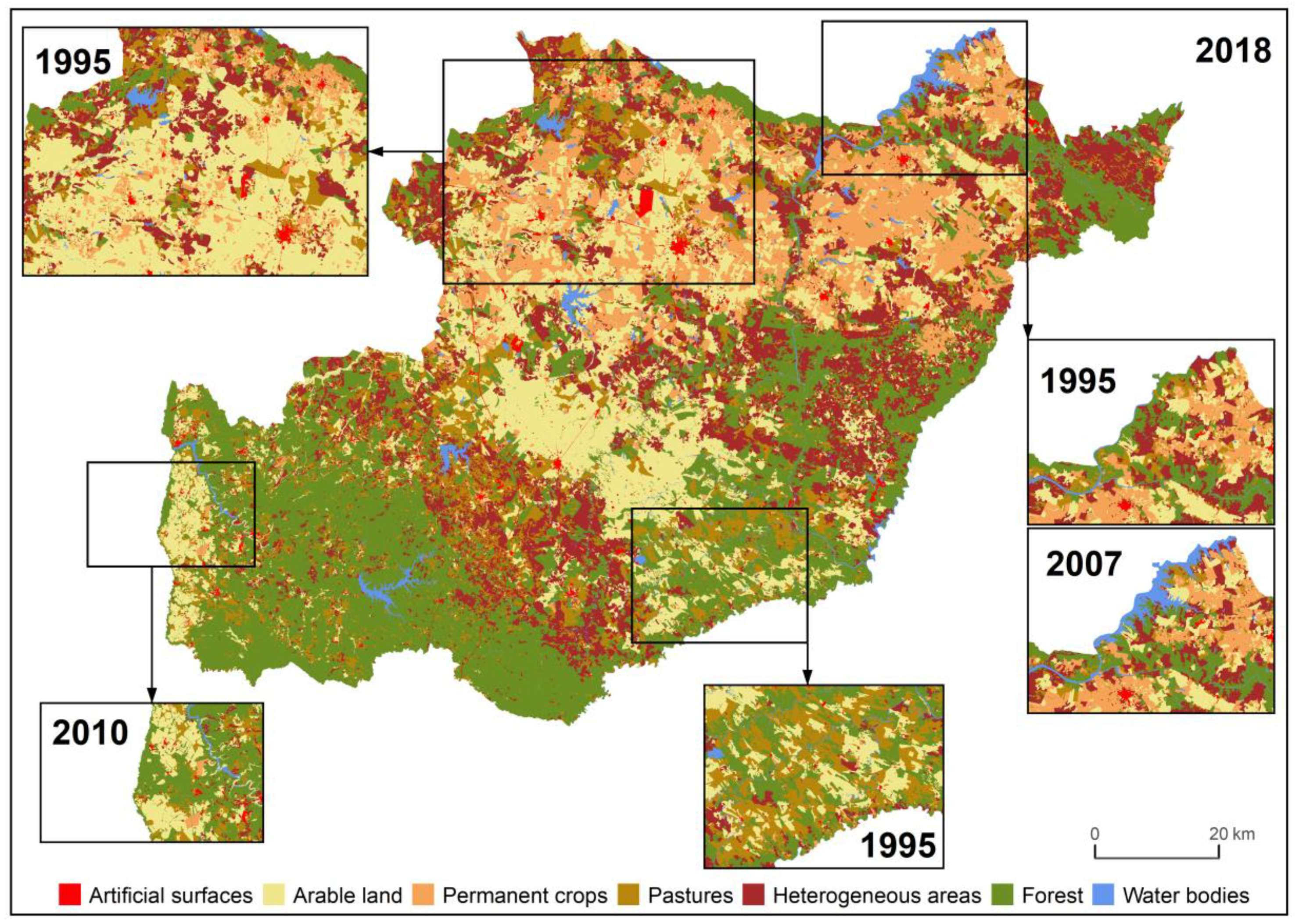
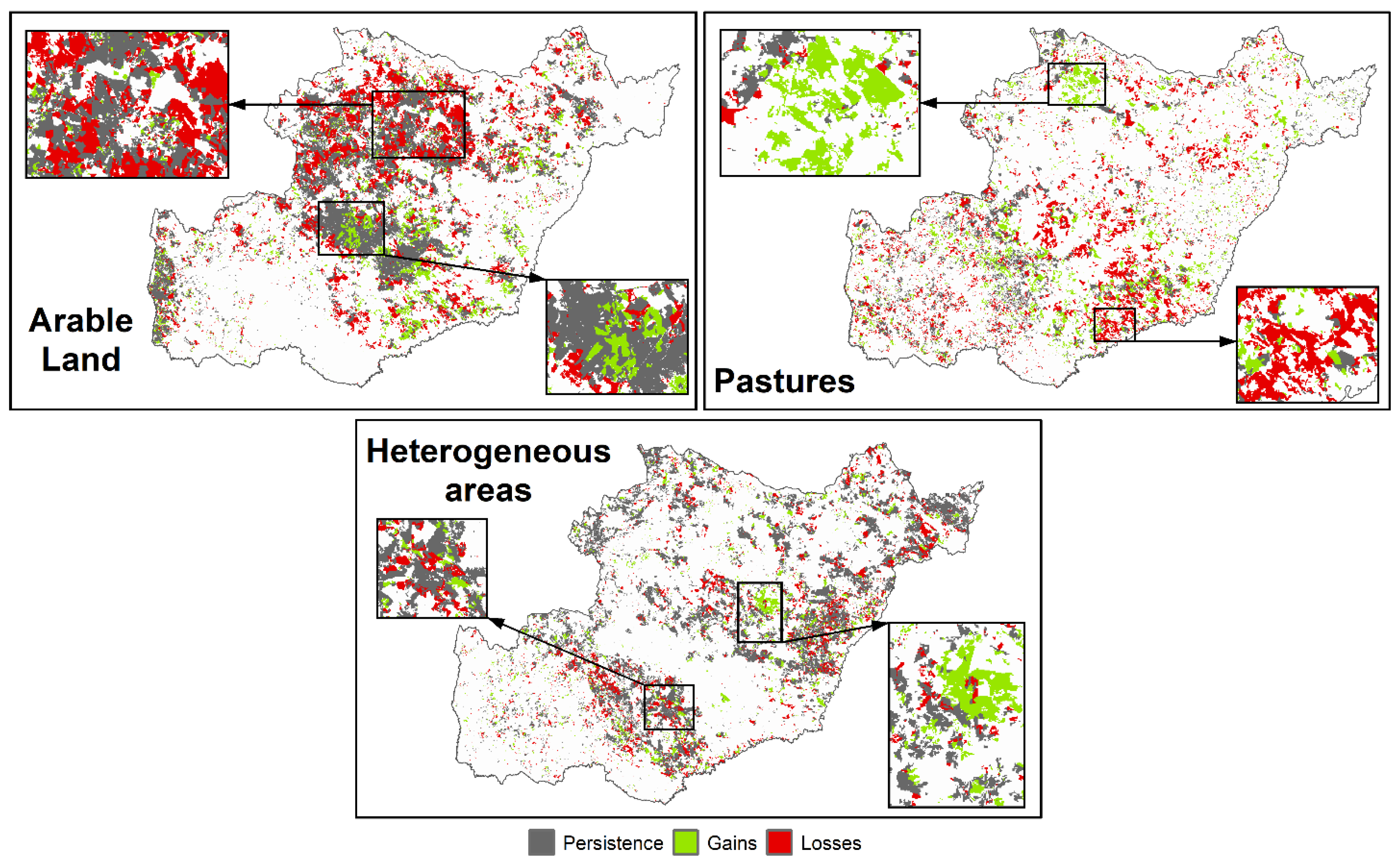
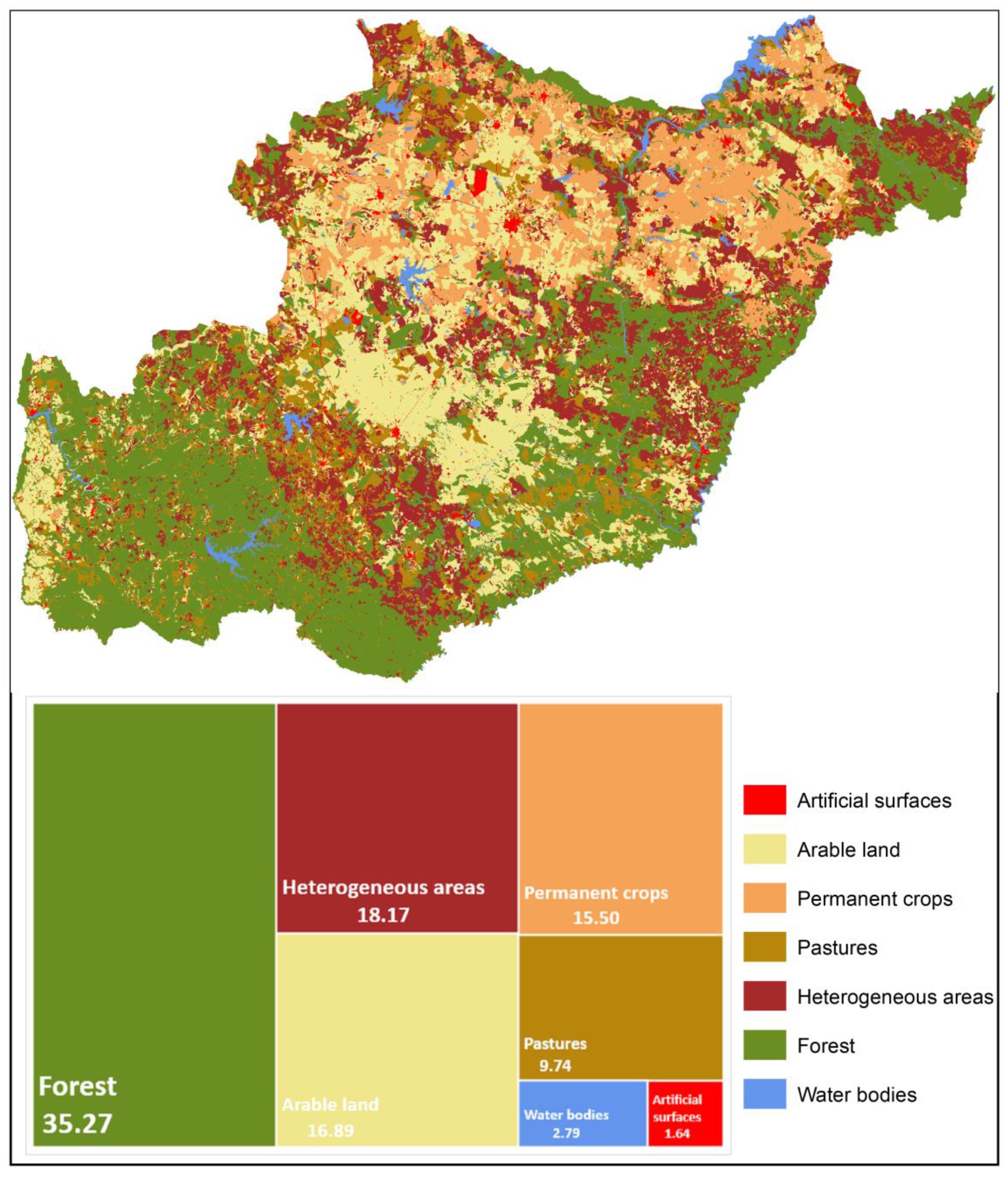
In 23 years, about 28% of the Beja district experienced dozens of inter-class transitions, but the most significant changes were in the croplands. Nevertheless, croplands remain the predominant LULC class in more than half of the Beja district (in 2018 about 64%). Particularly, there was a predominance of arable land that was dispersed in a great part of Beja, despite the significant decrease in this practice between 1995 and 2018 (−5.9%). Despite the decrease, the results confirmed the importance of cereal production in this region, as in the case of wheat [43,44]. Likewise, heterogeneous areas experienced a continuous decline (−2%), but even so this class represents the second largest cropland in the district, which confirms the relevance of the Montado system and the cork oak exploitation in the agroforestry areas of the district.
(ii)
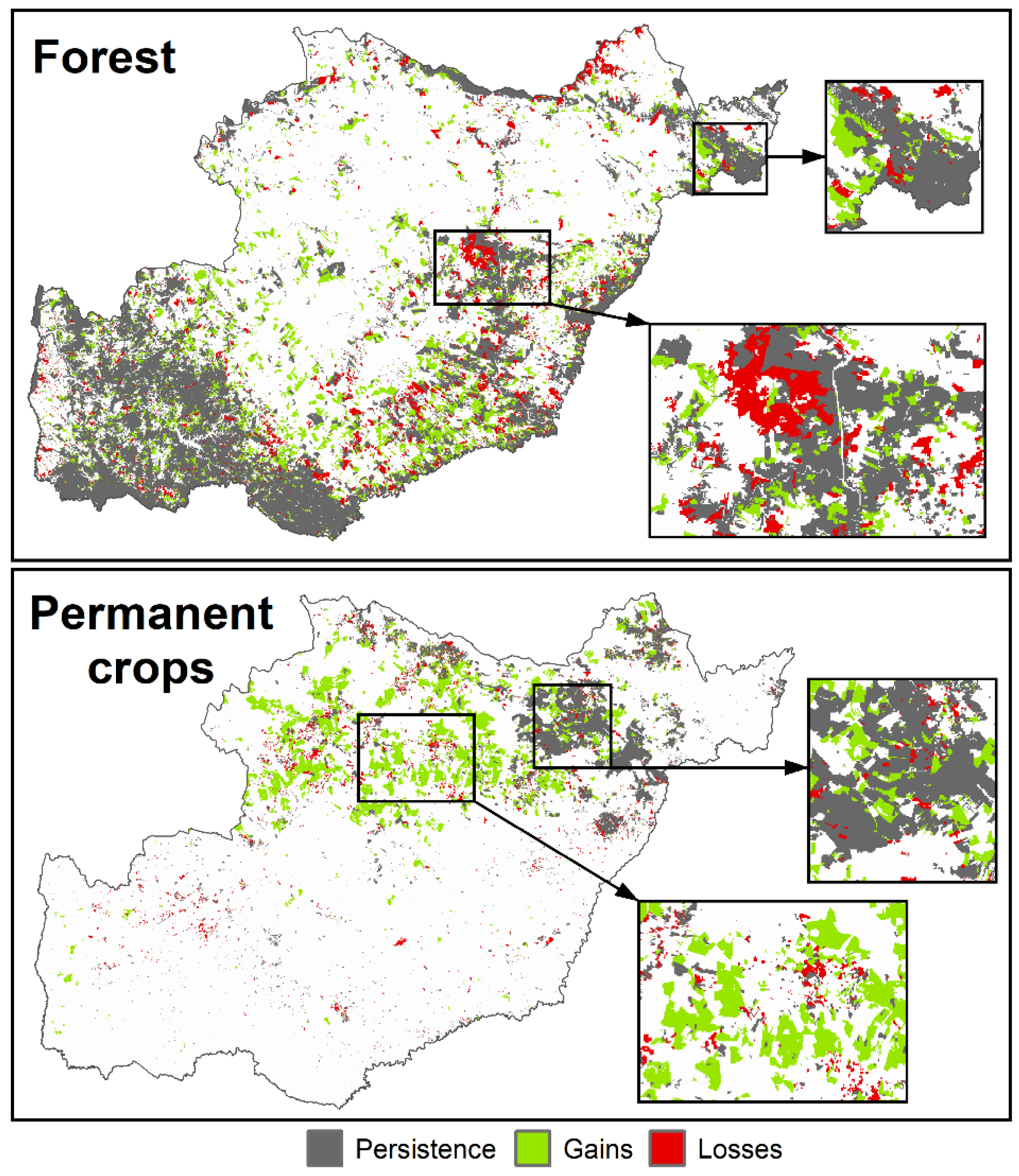
Of all the agricultural classes, permanent crops experienced a growing tendency. Thus, this cropland gained prevalence after a certain period and simultaneously experienced some loss (+5.13% between 1995 and 2018). In spite of the reduction in the territory, the substantial increase in permanent crops suggests an emphasis on intensive farming without fallow, proved by the enlargement of the olive grove plantation in this region and the increase in olive oil production [43,44]. These results are consistent with other studies, despite the methodological approach differences [31,32,45].
(iii)
As for the overall period, forests experienced more gains than losses (+4.31% between 1995 and 2018). There was a clear tendency of agricultural land loss to the detriment of forests, these results being in line with what is happening on a national level observed in other studies [30,46]. Additionally, about 63% of the total changes experienced by forests was attributed to a swap type, which may indicate that the Beja district simultaneously experienced forms of reforestation and deforestation between 1995 and 2018.
(iv)
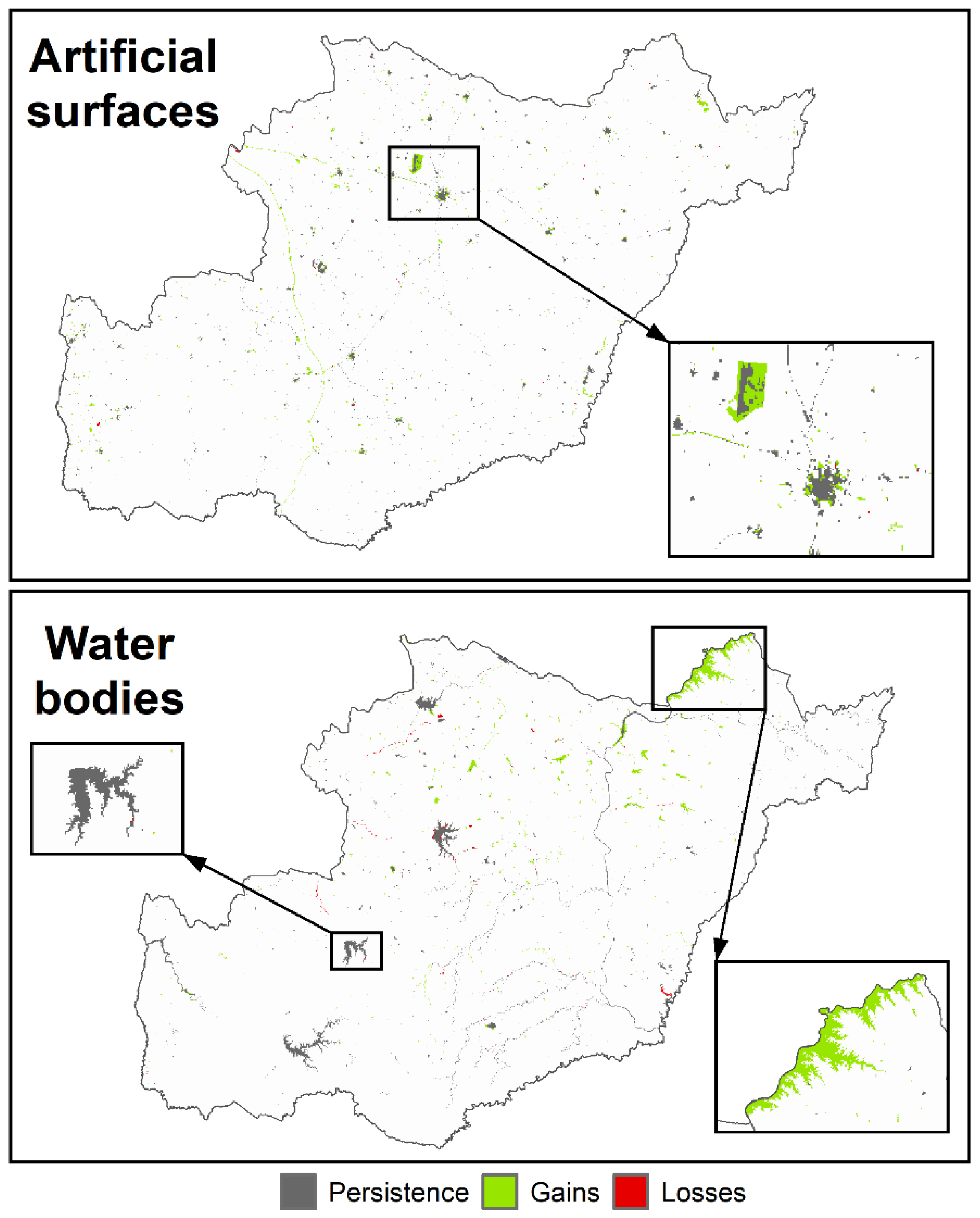
Lastly, artificial surfaces and water bodies experienced more gains than losses and showed a tendency to persist. A main cause for these observed gains is spatial conversions, such as the expansion of the Beja airport area and the construction of new roads in the case of artificial surfaces [47], and the Alqueva dam construction in 2002 in the case of the water bodies [31]. Nonetheless, artificial surfaces only increased about 0.45%, between 1995 and 2018, which indicates that the increase in urban areas was not remarkable in the Beja district, thereby counteracting the Portuguese trend towards an urban area increase [46].
Accordingly, the behavior of the inter-class transitions was significantly different between periods, and explicitly revealed that arable land, pastures, and forest were the most dynamic LULC classes, having experienced both damage and recovery over the years. Hence, the drivers that promote the LULC gains are likely to differ from the drivers that lead to LULC losses [12]. On the one hand, the main cause for cropland changes could be the competition between LULC classes, since such competition may restrict the use of available land even when this land has suitable determinants for a specific LULC class, which would explain higher observed losses compared with gains [12]. In addition, the political measures of incentives for the increase in technology, for example, the almost total abandonment of traditional agriculture or the high level of subsidies to agriculture, could be explanatory factors for the agricultural LULC changes observed [48]. Accordingly, the LULC periodical fluctuations were depolarized by certain drivers, such as political decisions, economic development planning, or even weather conditions, showing the importance of the analysis of the possible drivers of changes in future work [46].

4.2. About the Dominant LULC Transitions

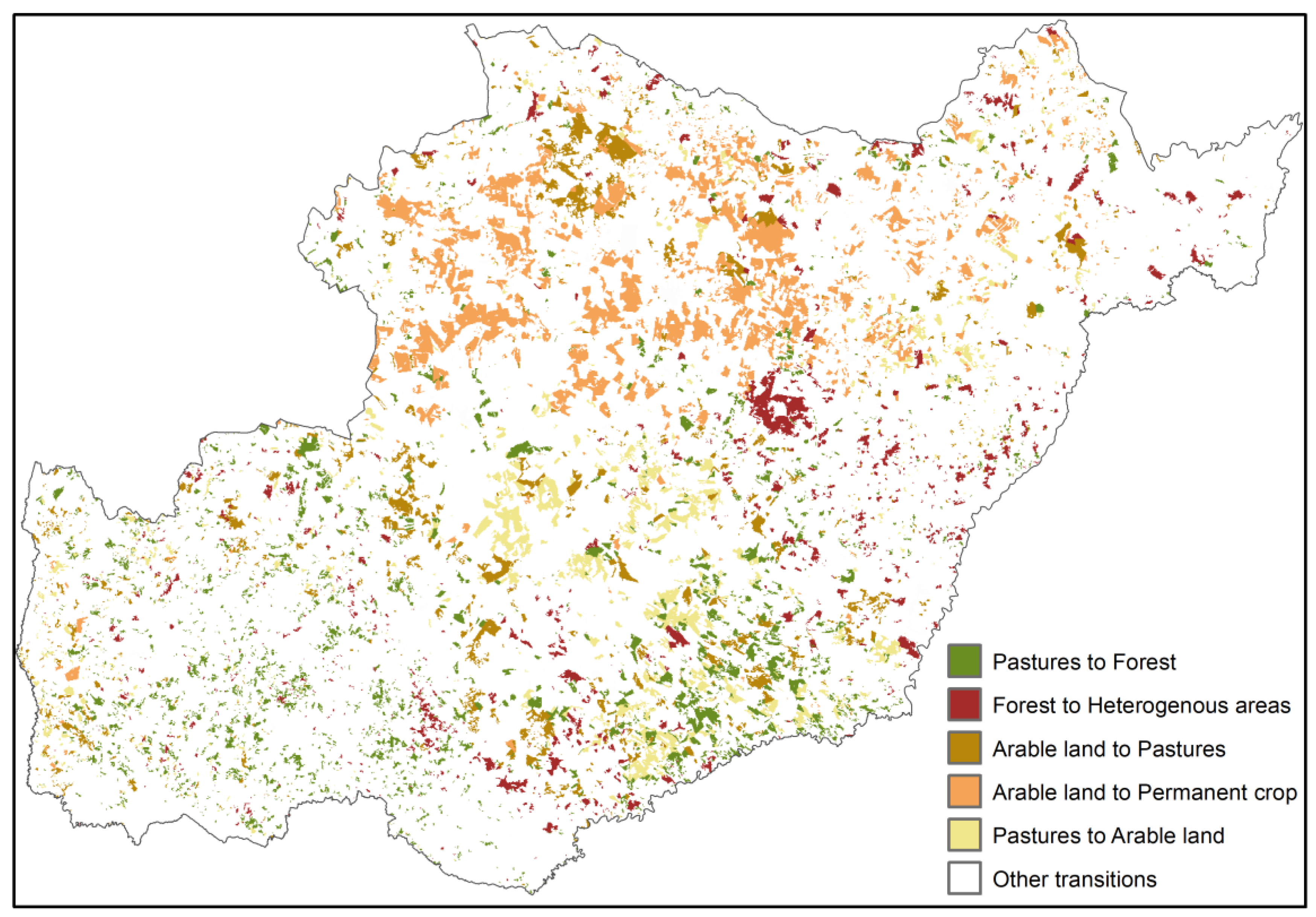
The analysis of the differences between the observed LULC and the expected LULC gains and losses under a random process of changes showed that, of the several observed inter-class transitions, few experienced dominant signals of change between 1995 and 2018 (Figure 11), namely:
(i)
transitions of arable land to permanent crops and to pastures, which accounted for about 5% and 2.9%, respectively;
(ii)
transitions of pastures to forest and arable land, which accounted for about 3.5% and 2.7%, respectively;
(iii)
transitions of forest to heterogeneous areas, which accounted for about 2.1%.
Accordingly, the arable land tendency to lose, especially for the permanent crops class, causes some concerns. The Beja district located in the Mediterranean region is a suitable region to produce olive oil mainly due to favorable weather conditions. Moreover, the positive market environment prevailed with the gradual increase in global olive oil consumption in the past decade, and the super-intensive olive grove plantation also increased to cover the demand [45]. Thus, traditional olive grove plantations are becoming unusual, mainly because the super-intensive cropland production profitability is higher and because of Common Agricultural Policy (CAP) incentives [49]. While this type of agricultural practice will start producing in the 3rd year after planting, the traditional practice can occur after one decade. In addition, mechanization in the super-intensive olive grove is less labor-dependent, meaning a greater capacity for profit. Hence, this all points to one conclusion: the high increase in super-intensive olive crops to produce olive oil is highly associated with the expansion of permanent crops, which is at the expense of arable land.
Thus, the Beja district is experiencing a new landscape dynamic, caused not only by the systematic increase in permanent crops areas but also by the decrease of arable land that produces a historical agricultural product: wheat (the grain of civilization). Indeed, over the last century, Beja consistently showed remarkable importance in wheat production, mainly explained by: (i) the type of soil in Beja, “Barros de Beja” (Beja clays), which is a dense and deep soil that is particularly suitable for this cereal production; (ii) the type of land exploitation (latifundium) [50]; and (iii) the weather conditions (i.e., a temperate climate with Mediterranean characteristics), as the wheat crop has a relative tolerance to water deficiency [51].
Thus, these results indicate that, although arable land predominated in the Beja district between 1995 and 2018, this cropland experienced a significant decrease due to the competition between LULC classes. Accordingly, the transition from arable land to permanent crops was relatively constant over time, and it was more pronounced in the last period (2015–2018), presumably triggered by the substantial increase of foreign investment (especially from Spanish investors) and the strong exploitation of water resources, after the construction of the Alqueva dam that filled its reservoir only 10 years after construction began (in 2012) [45]. Thus, it seems essential to assess the impact of this systematic transition, since everything points to an increasing super-intensive olive grove cultivation system that will result in a negative impact on this land in the future [52].
In addition, arable land also experienced systematic transitions to pastures. This change was especially strong in the first period (1995–2007), possibly due to changes in the CAP, which led to a decrease in the areas under arable crops, in particular cereal production, and an increase in fallow land maintenance and natural pasture. These policies arose out of a concern related to land preservation in the context of rural planning, resulting, among other actions, in reduced dryland cereal cultivation areas, due to the recognition of the negative impact on soil depletion and erosion resulting from previous agricultural campaigns [53] and an international acknowledgement of the role of such areas in mitigating climate change [54,55].
On the contrary, Beja also experienced a systematic transition from pastures to arable land. This dynamic LULC change was substantially stronger in the first period (1995–2007) and partly contradicts the prior interpretation of the possible factors responsible for such changes. Therefore, following the abovementioned explanations, we believe this transition can also be linked with the implementation of the CAP, which favors fallow land maintenance. Indeed, the arable land class mainly comprises a land rotation system between annually harvested crops (rain-fed or irrigated) and fallow plots, which in our study area mainly represents dry-fed and rain-fed cereal production. However, according to the COS map nomenclature, this class can also comprise fallow land for a maximum of five years. Additionally, agricultural pasture systems have limitations regarding their production irregularity over a given year due to the irregularity of rainfall [56,57] and may not be economically viable for farmers if not subsidized [50,58], which may partly justify these changes in the landscape.
In the Beja district, a systematic transition from pastures to forestland was also found, and this was most significant in the first period (1995–2007) and was probably associated with afforestation policy (the 1992 CAP reform) and EU subsidies (Agenda 2000), which promoted the conversion of pastures in Eucalyptus and Pinus forests [50] for conservation of the land’s structure and functions. Lastly, the systematic transition from forest to heterogeneous areas, which occurred significantly between the third period (2010–2015), is probably related to forest fires, as reforestation took place after this event in the form of Montado to combat desertification [59].
For instance, the examination of the systematic and random transition showed that some of the major LULC transitions, such as heterogeneous areas and arable land transitioning to forest (2.53% and 1.78%, respectively) and the heterogeneous areas transitioning to pastures (1.18%), were random or partially systematic. In addition, it is interesting that heterogeneous areas did not experience systematic losses, which indicates a strong signal of persistence in this LULC class. Thus, the Beja district still retains important traditional agricultural areas, such as the Montado, an agrosilvopastoral system of global importance.

4.3. About the LULC Future Changes

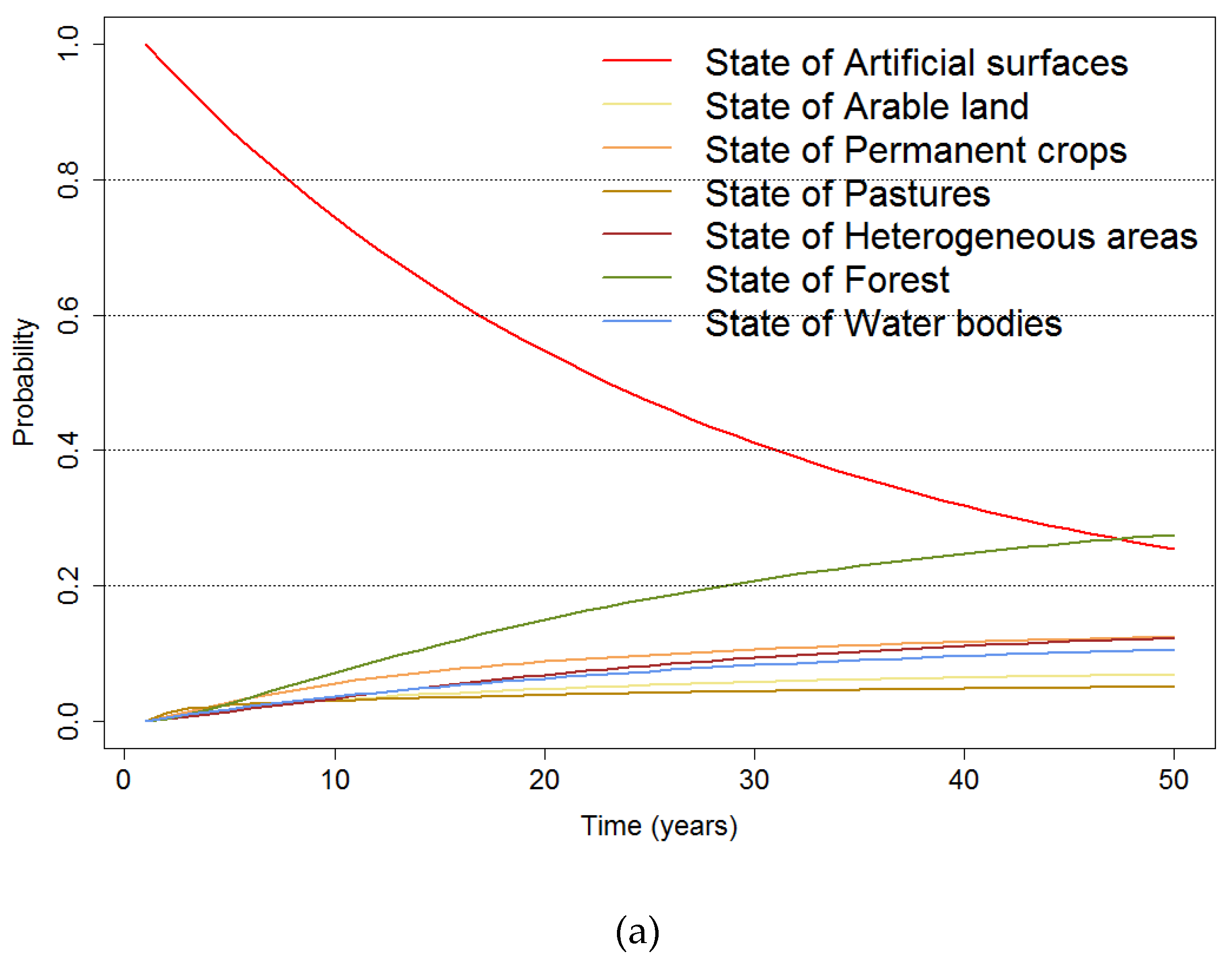
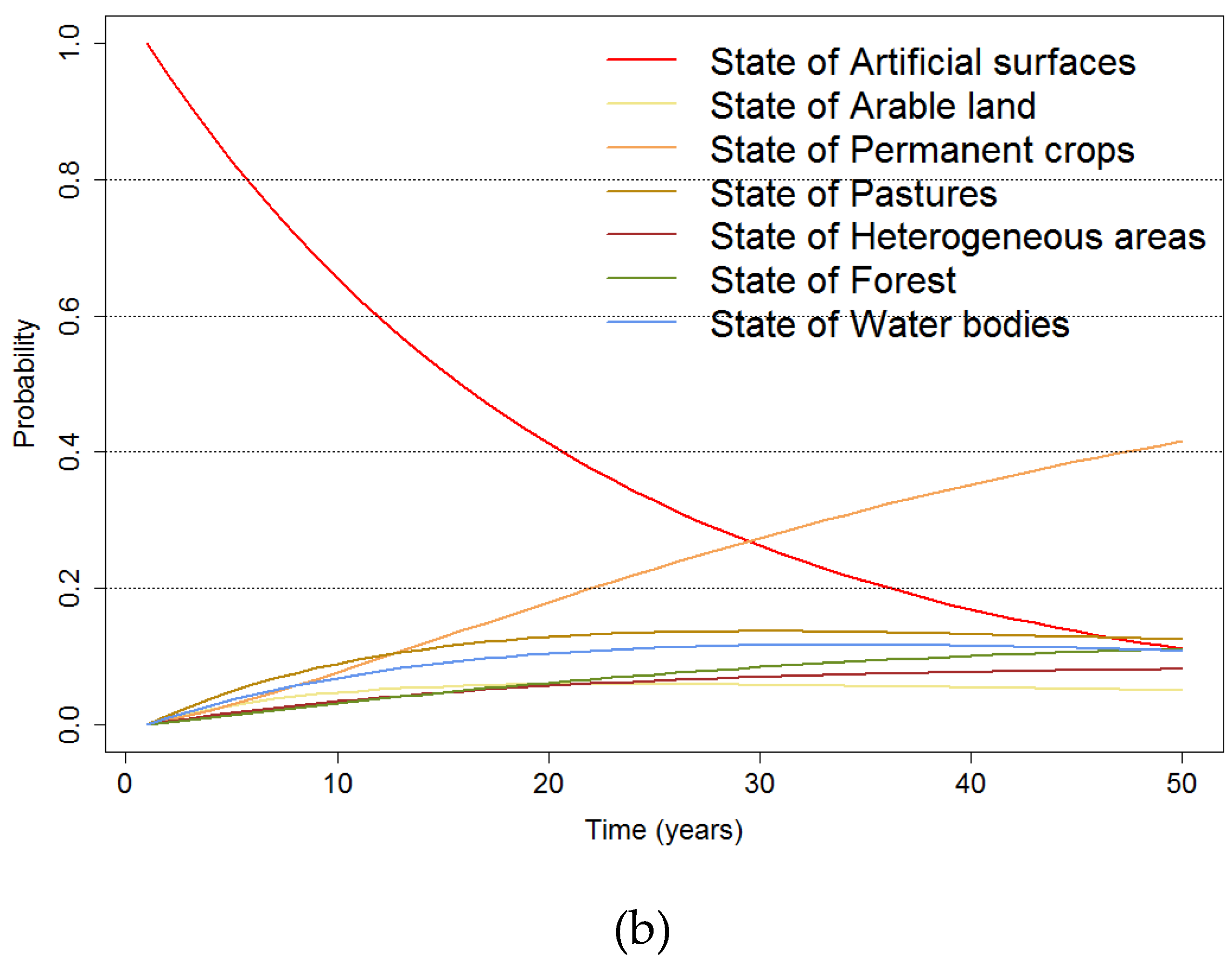
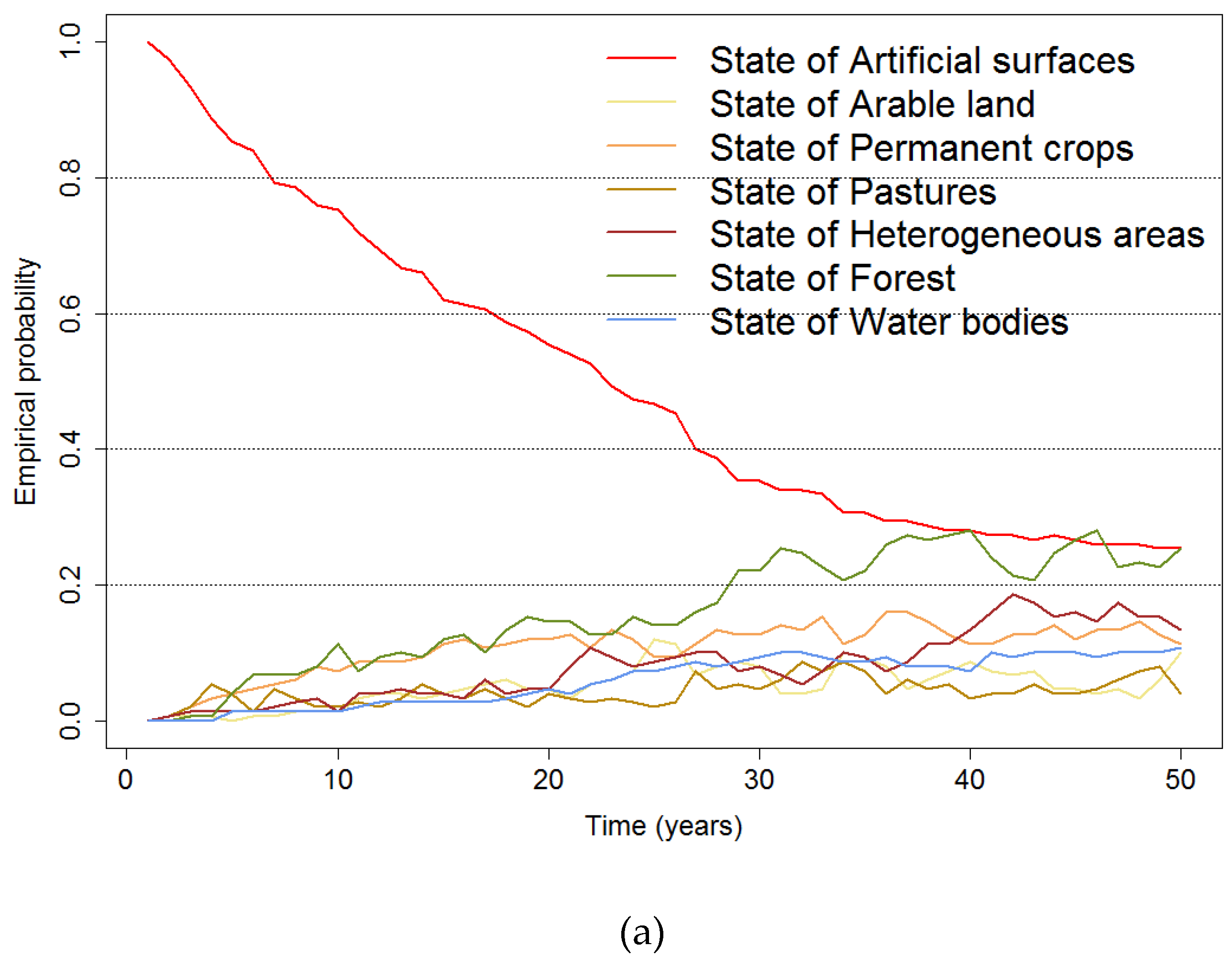
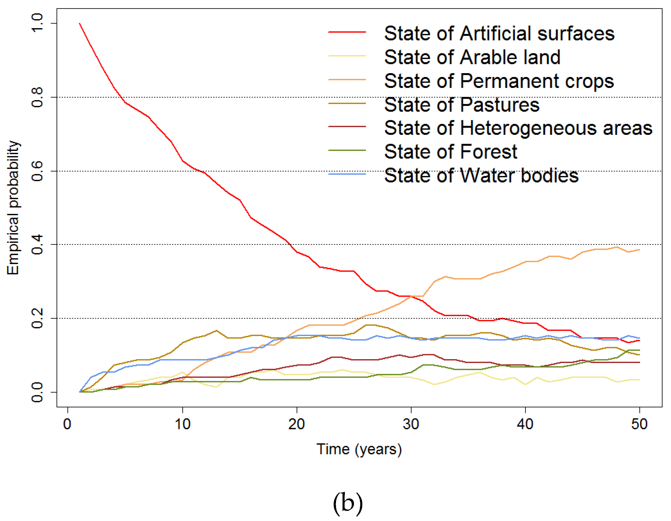
The transition probability simulation between uses for the year 2040 allowed us to understand that imbalances can arise in the future, highlighting that about 25% of the territory is predicted to transition, and about 21% of that territory corresponds to agricultural land. These results are a warning that the Beja district will experience strong landscape dynamics in agricultural land, emphasizing the importance of measures in mitigating the negative effects of such strong signals of LULC transitions [12].
Additionally, the DTMC model showed a high agreement value, proving to be a useful mechanism for monitoring and evaluating LULC changes, with a trend projection with high applicability and flexibility. Therefore, the main advantage of using Markov chains is their mathematical logic that enables swift applications, as well as their possible interaction with other techniques such as remote sensing and GIS, both of which commonly work with matrices. However, a disadvantage of this model is that it does not explain the facts, because the process only takes into account the time variable. Thus, predictions made through this model mostly indicate changes in the state of variables in time and not in space. Nevertheless, the stationary probabilities are useful as indicators of the landscape shares of each LULC class and provide highly valuable information in decision-making processes.

4.4. Main Conclusions and Future Studies

The purpose of this study was to analyze the spatiotemporal evolution of LULC in Beja from 1995 to 2018 and simulate the future development for the year 2040. This analysis indicates that in 23 years there were significant changes that deeply modify the Beja district landscape, mainly due to two opposite phenomena: the intensification of agricultural practices and the afforestation of agricultural lands. The observed LULC patterns reflect the last decade’s structural changes in the Portuguese economy and society and confirm the impact of political decisions and different agricultural activity management, which led to the loss of a significant amount of agricultural heritage. In fact, this regional landscape and the traditional features of agricultural land are facing an uneven transformation dynamic that does not take into account either the balance or the environmental enhancement of the local diversity agricultural systems [49].
The acquired spatiotemporal knowledge regarding the agricultural LULC changes allowed us to obtain a general picture of the main transitions of a region of Portugal that has more importance in the regional agricultural production sector, particularly in the production of cereals, such as wheat, barley, oats, and other products such as olive oil and cork. An understanding of the systematic transitions and the locations thereof provides useful insight into ecosystem service management and contributes to future sustainability strategies. Nonetheless, this statistical approach is exclusively based on an analysis of the LULC transition matrix, and the interpretation of the LULC transitions is based on a sequence of historical determinism documented in prior investigations (e.g., [49,57,60]), so any factor mentioned to rationalize the systematic transition is based only on assumptions of historical fact. Therefore, additional research is necessary to assess the many processes that create these LULC changes, which have been linked to dozens of possible drivers and their different levels of feedback. Still, providing an understanding of the inter-class transitions that have occurred as systematic changes has proven to be a straightforward, effective approach that allows us to differentiate the predominating quantity transitions from those that experienced a single abrupt episode process of change influenced by factors that occur suddenly.
The information obtained contributed to sciences related to the earth and human society on a variety of levels, providing effective information for economic and environmental monitoring and evaluation, resulting in informed policy decisions and in the design of anticipatory measures response to change. Furthermore, in this exploratory study, we used COS maps, official Portuguese LULC data produced by a governmental institution (DGT), and these data were advantageous because of their higher cartographic detail and were characterized by temporal continuity. This highlights the importance of having an entity responsible for producing LULC thematic cartography with regularity and reliability and making it available free of charge, as it can be used for multiple purposes, such as territorial planning and management, ecosystem service mapping, and the identification of areas vulnerable to rural fires (e.g., [34,61,62,63]).

Author Contributions

Conceptualization, C.M.V. and J.R.; methodology & software, C.M.V. and J.R.; data curation, C.M.V.; validation, C.M.V. and J.R.; formal analysis, C.M.V.; investigation, C.M.V.; writing—original draft preparation, C.M.V; writing—review and editing, C.M.V. and J.R. All authors have read and agreed to the published version of the manuscript.

Funding

This research was funded by the Portuguese Foundation for Science and Technology (FCT) [grant number SFRH/BD/115497/2016 to Cláudia M. Viana] and by the Centre for Geographical Studies—Universidade de Lisboa and FCT [grant number UID/GEO/00295/2019].

Acknowledgments

We acknowledge the GEOMODLAB—Laboratory for Remote Sensing, Geographical Analysis and Modelling—of the Center of Geographical Studies/IGOT for providing the required equipment and software. The authors would also like to thank to the editor and the three anonymous reviewers that contributed to the improvement of this paper.

Conflicts of Interest

The authors declare no conflict of interest.

References

  1. Feranec, J.; Soukup, T.; Taff, G.; Stych, P.; Bicik, I. Overview of changes in land cover and land use in Eastern Europe. In Land-Cover and Land-Use Changes in Eastern Europe after the Collapse of the Soviet Union in 1991; Gutman, G., Radeloff, V., Eds.; Springer: Berlin, Germany, 2017. [Google Scholar]
  2. Fuchs, R.; Herold, M.; Verburg, P.H.; Clevers, J.G.P.W.; Eberle, J. Gross changes in reconstructions of historic land cover/use for Europe between 1900 and 2010. Glob. Chang. Biol. 2015, 21, 299–313. [Google Scholar] [CrossRef] [PubMed]
  3. Turner, B.; Moss, R.H.; Skole, D.L. Relating Land Use and Global Land-Cover Change—IGBP Report No. 24, HDP Report No. 5; International Geosphere-Biosphere Programme (IGBP) Secretariat, Royal Swedish Academy of Sciences: Stockholm, Sweden, 1993. [Google Scholar]
  4. Deng, X.; Huang, J.; Rozelle, S.; Uchida, E. Growth, population and industrialization, and urban land expansion of China. J. Urban Econ. 2008, 63, 96–115. [Google Scholar] [CrossRef]
  5. Lu, Q.; Liang, F.; Bi, X.; Duffy, R.; Zhao, Z. Effects of urbanization and industrialization on agricultural land use in Shandong Peninsula of China. Ecol. Indic. 2011, 11, 1710–1714. [Google Scholar] [CrossRef]
  6. Hansen, M.C.; Loveland, T.R. A review of large area monitoring of land cover change using Landsat data. Remote Sens. Environ. 2012, 122, 66–74. [Google Scholar] [CrossRef]
  7. Uddin, K.; Matin, M.A.; Maharjan, S. Assessment of land cover change and its impact on changes in soil erosion risk in Nepal. Sustainability 2018, 10, 4715. [Google Scholar] [CrossRef] [Green Version]
  8. Rousta, I.; Sarif, M.O.; Gupta, R.D.; Olafsson, H.; Ranagalage, M.; Murayama, Y.; Zhang, H.; Mushore, T.D. Spatiotemporal analysis of land use/land cover and its effects on surface urban heat Island using landsat data: A case study of Metropolitan City Tehran (1988–2018). Sustainability 2018, 10, 4433. [Google Scholar] [CrossRef] [Green Version]
  9. Mertens, B.; Sunderlin, W.D.; Ndoye, O.; Lambin, E.F. Impact of macroeconomic change on deforestation in South Cameroon: Integration of household survey and remotely-sensed data. World Dev. 2000, 28, 983–999. [Google Scholar] [CrossRef]
  10. Petit, C.; Scudder, T.; Lambin, E. Quantifying processes of land-cover change by remote sensing: Resettlement and rapid land-cover changes in south-eastern Zambia. Int. J. Remote Sens. 2001, 22, 3435–3456. [Google Scholar] [CrossRef]
  11. Pontius, R.G.; Shusas, E.; Mceachern, M. Detecting important categorical land changes while accounting for persistence. Agric. Ecosyst. Environ. 2004, 101, 251–268. [Google Scholar] [CrossRef]
  12. Braimoh, A.K. Random and systematic land-cover transitions in northern Ghana. Agric. Ecosyst. Environ. 2006, 113, 254–263. [Google Scholar] [CrossRef]
  13. Lambin, E.F.; Geist, H.J.; Lepers, E. Dynamics of Land-use and Land-cover change in tropical regions. Annu. Rev. Environ. Resour. 2003, 28, 205–241. [Google Scholar] [CrossRef] [Green Version]
  14. Teferi, E.; Bewket, W.; Uhlenbrook, S.; Wenninger, J. Understanding recent land use and land cover dynamics in the source region of the Upper Blue Nile, Ethiopia: Spatially explicit statistical modeling of systematic transitions. Agric. Ecosyst. Environ. 2013, 165, 98–117. [Google Scholar] [CrossRef]
  15. Deribew, K.T. Spatially explicit statistical modeling of random and systematic land cover transitions in the main grassland plain of Nech Sar National Park, Ethiopia. Ecol. Process. 2019, 8, 46. [Google Scholar] [CrossRef]
  16. Hyandye, C.; Martz, L.W. A Markovian and cellular automata land-use change predictive model of the Usangu Catchment. Int. J. Remote Sens. 2017, 38, 64–81. [Google Scholar] [CrossRef]
  17. Han, H.; Yang, C.; Song, J. Scenario simulation and the prediction of land use and land cover change in Beijing, China. Sustainability 2015, 7, 4260–4279. [Google Scholar] [CrossRef] [Green Version]
  18. Yirsaw, E.; Wu, W.; Shi, X.; Temesgen, H.; Bekele, B. Land Use/Land Cover Change Modeling and the Prediction of Subsequent Changes in Ecosystem Service Values in a Coastal Area of China, the Su-Xi-Chang Region. Sustainability 2017, 9, 1204. [Google Scholar] [CrossRef] [Green Version]
  19. Agarwal, C.; Green, G.M.; Grove, J.M.; Evans, T.P.; Schweik, C.M. A Review and Assessment of Land-Use Change Models: Dynamics of Space, Time, and Human Choice. Apollo Int. Mag. Art Antiq. 2002, 62. [Google Scholar] [CrossRef] [Green Version]
  20. Gagniuc, P.A. Markov Chains: From Theory to Implementation and Experimentation; John Wiley & Sons: Hoboken, NJ, USA, 2017; ISBN 9781119387558. [Google Scholar]
  21. Hathout, S. The use of GIS for monitoring and predicting urban growth in East and West St Paul, Winnipeg, Manitoba, Canada. J. Environ. Manag. 2002, 66, 229–238. [Google Scholar] [CrossRef]
  22. Weng, Q. Land use change analysis in the Zhujiang Delta of China using satellite remote sensing, GIS and stochastic modelling. J. Environ. Manag. 2002, 64, 273–284. [Google Scholar] [CrossRef] [Green Version]
  23. Liu, Y.; Feng, Y. Simulating the Impact of Economic and Environmental Strategies on Future Urban Growth Scenarios in Ningbo, China. Sustainability 2016, 8, 1045. [Google Scholar] [CrossRef] [Green Version]
  24. Hamad, R.; Balzter, H.; Kolo, K. Predicting land use/land cover changes using a CA-Markov model under two different scenarios. Sustainability 2018, 10, 3421. [Google Scholar] [CrossRef] [Green Version]
  25. Li, X.; Yeh, A.G.-O. Neural-network-based cellular automata for simulating multiple land use changes using GIS. Int. J. Geogr. Inf. Sci. 2002, 16, 323–343. [Google Scholar] [CrossRef]
  26. Iacono, M.; Levinson, D.; El-Geneidy, A.; Wasfi, R. A Markov Chain Model of Land Use Change in the Twin Cities, 1958-2005. Tema. J. L. Use, Mobil. Environ. 2015; 8, 263–276. [Google Scholar] [CrossRef]
  27. Ahmed, B.; Ahmed, R.; Zhu, X. Evaluation of model validation techniques in land cover dynamics. ISPRS Int. J. Geo Inf. 2013, 2, 577–597. [Google Scholar] [CrossRef]
  28. Basharin, G.P.; Langville, A.N.; Naumov, V.A. The life and work of A.A. Markov. Linear Algebra Appl. 2004, 386, 3–26. [Google Scholar] [CrossRef] [Green Version]
  29. Pinto-Correia, T. Future development in Portuguese rural areas: How to manage agricultural support for landscape conservation? Landsc. Urban Plan. 2000, 50, 95–106. [Google Scholar] [CrossRef]
  30. Feranec, J.; Jaffrain, G.; Soukup, T.; Hazeu, G. Determining changes and flows in European landscapes 1990–2000 using corine land cover data. Appl. Geogr. 2010, 30, 19–35. [Google Scholar] [CrossRef]
  31. Allen, H.; Simonson, W.; Parham, E.; Santos, E.d.B.e.; Hotham, P. Satellite remote sensing of land cover change in a mixed agro-silvo-pastoral landscape in the Alentejo, Portugal. Int. J. Remote Sens. 2018, 39, 4663–4683. [Google Scholar] [CrossRef]
  32. Viana, C.M.; Girão, I.; Rocha, J. Long-term satellite image time-series for land use/land cover change detection using refined open source data in a rural region. Remote Sens. 2019, 11, 1104. [Google Scholar] [CrossRef] [Green Version]
  33. Tavares, A.O.; Pato, R.L.; Magalhães, M.C. Spatial and temporal land use change and occupation over the last half century in a peri-urban area. Appl. Geogr. 2012, 34, 432–444. [Google Scholar] [CrossRef]
  34. Meneses, B.M.; Reis, E.; Vale, M.J.; Reis, R. Modelling the Land Use and Land cover changes in Portugal: A multi-scale and multi-temporal approach. Finisterra 2018, 53. [Google Scholar] [CrossRef]
  35. Muñoz-Rojas, J.; Pinto-Correia, T.; Hvarregaard Thorsoe, M.; Noe, E. The Portuguese Montado: A Complex System under Tension between Different Land Use Management Paradigms. In Silvicultures—Management and Conservation; IntechOpen: London, UK, 2019. [Google Scholar]
  36. Correia, T.P. Threatened landscape in Alentejo, Portugal: The “montado” and other “agro-silvo-pastoral” systems. Landsc. Urban Plan. 1993, 24, 43–48. [Google Scholar] [CrossRef]
  37. Koohafkan, P.; Altieri, M.A. Forgotten Agricultural Heritage: Reconnecting Food Systems and Sustainable Development; Taylor & Francis: London, UK, 2016; ISBN 9781138204157. [Google Scholar]
  38. INE. Censos 2011 Resultados Definitivos—Região Alentejo; Instituto Nacional de Estatística: Lisboa, Portugal, 2012; ISBN 978-989-25-0182-6. (In Portuguese) [Google Scholar]
  39. DGT. Especificações Técnicas da Carta de Uso e Ocupação do Solo (COS) de Portugal Continental Para 1995, 2007, 2010 e 2015; DGT: Madrid, Spain, 2018. (In Portuguese) [Google Scholar]
  40. Pontius, R.G.; Boersma, W.; Castella, J.C.; Clarke, K.; Nijs, T.; Dietzel, C.; Duan, Z.; Fotsing, E.; Goldstein, N.; Kok, K.; et al. Comparing the input, output, and validation maps for several models of land change. Ann. Reg. Sci. 2008, 42, 11–37. [Google Scholar] [CrossRef] [Green Version]
  41. Shi, W.; Fisher, P.F.; Goodchild, M.F. Spatial Data Quality; Taylor & Francis: London, UK, 2002; ISBN 0-415-25835-9. [Google Scholar]
  42. Van der Wel, F.J.M.; Van der Gaag, L.C.; Gorte, B.G.H. Visual exploration of uncertainty in remote-sensing classification. Comput. Geosci. 1998, 24, 335–343. [Google Scholar] [CrossRef] [Green Version]
  43. Viana, C.M.; Freire, D.; Rocha, J. Regional agricultural production statistics for 160 years using the geographic information system and the spatial analytical technique. In Geospatial Technologies for Local and Regional Development: Short Papers, Posters and PosterAbstracts of the 22th AGILE Conference on Geographic Information Science, Limassol, Cyprus, 17–20 June 2019; Kyriakidis, P., Hadjimitsis, D., Skarlatos, D., Mansourian, A., Eds.; Cyprus University of Technology: Limassol, Cyprus, 2019. [Google Scholar]
  44. Viana, C.M.; Rocha, J. Spatiotemporal analysis and scenario simulation of agricultural land use land cover using GIS and a Markov chain model. In Geospatial Technologies for All: Short Papers, Posters and Poster Abstracts of the 21th AGILE Conference on Geographic Information Science, Lund, Sweden, 12–15 June 2018; Mansourian, A., Pilesjö, P., Harrie, L., von Lammeren, R., Eds.; Lund University: Lund, Sweden, 2018. [Google Scholar]
  45. Roxo, M.J.; Ventura, J.E. Land Use Change in the Lower Alentejo (South of Portugal) and the New Environmental Challenges: The Olive Culture. In Environment and Ecology in the Mediterranean Region; Efe, R., Ozturk, M., Ghazanfa, S., Eds.; Cambridge Scholars Publishing: Newcastle upon Tyne, UK, 2012; pp. 13–28. ISBN 978-1-4438-3757-6. [Google Scholar]
  46. Meneses, B.M.; Reis, E.; Pereira, S.; Vale, M.J.; Reis, R. Understanding driving forces and implications associated with the land use and land cover changes in Portugal. Sustainability 2017, 9, 9–14. [Google Scholar] [CrossRef] [Green Version]
  47. Viana, C.M.; Oliveira, S.; Oliveira, S.C.; Rocha, J. Land Use/Land Cover Change Detection and Urban Sprawl Analysis. In Spatial Modeling in GIS and R for Earth and Environmental Sciences; Pourghasemi, H.R., Gokceoglu, C., Eds.; Elsevier: Amsterdam, The Netherlands, 2019; ISBN 9780128152263. [Google Scholar]
  48. Serra, P.; Pons, X.; Saurí, D. Land-cover and land-use change in a Mediterranean landscape: A spatial analysis of driving forces integrating biophysical and human factors. Appl. Geogr. 2008, 28, 189–209. [Google Scholar] [CrossRef]
  49. De Ferreira, D.B. Evolução Da Paisagem De Montado No Alentejo Interior Ao Longo Do Século XX: Dinâmica e incidências ambientais. Finisterra 2001, 36, 179–193. (In Portuguese) [Google Scholar] [CrossRef] [Green Version]
  50. Jones, N.; de Graaff, J.; Rodrigo, I.; Duarte, F. Historical review of land use changes in Portugal (before and after EU integration in 1986) and their implications for land degradation and conservation, with a focus on Centro and Alentejo regions. Appl. Geogr. 2011, 31, 1036–1048. [Google Scholar] [CrossRef]
  51. Freire, D.; Lains, P. An Agrarian History of Portugal, 1000–2000: Economic Development on the European Frontier; Freire, D., Lains, P., Eds.; Brill: Leiden/Boston, MA, USA, 2017. [Google Scholar]
  52. García-Ruiz, J.M.; Nadal-Romero, E.; Lana-Renault, N.; Beguería, S. Erosion in Mediterranean landscapes: Changes and future challenges. Geomorphology 2013, 198, 20–36. [Google Scholar] [CrossRef] [Green Version]
  53. Serrano, J.E. Pastagens do Alentejo: Bases Técnicas Sobre Caracterização, Pastoreio e Melhoramento; de Icam, U.É., Ed.; Gráfica Eborense: Évora, Portugal, 2006. (In Portuguese) [Google Scholar]
  54. Thomas, R.J.; Lascano, C.E.; Sanz, J.I.; Ara, M.A.; Spain, J.M.; Vera, R.R.; Fisher, M.J. The Role of Pastures in Production Systems; Centro Internacional de Agricultura Tropical (CIAT): Cali, Colombia, 1992. [Google Scholar]
  55. Sevov, A.; Yancheva, C.; Kazakova, Y. Sustainable Pasture Management. In New Perspectives in Forage Crops; InTech: London, UK, 2018. [Google Scholar]
  56. Cosentino, S.L.; Gresta, F.; Testa, G. Forage chain arrangement for sustainable livestock systems in a Mediterranean area. Grass Forage Sci. 2013, 69, 625–634. [Google Scholar] [CrossRef]
  57. Ferreira, D.B. Problemas florestais no Alentejo: A crise do montado e a eucaliptização. Finisterra 1992, 27, 25–62. (In Portuguese) [Google Scholar] [CrossRef]
  58. Pearson, S.; Avillez, F.; Bentley, J.W. Portuguese Agriculture in Transition; Cornell University PressIthaca/Cornell University Press: Ithaca, NY, USA, 1987; ISBN 0801419549. [Google Scholar]
  59. Botequim, B.; Arias-Rodil, M.; Garcia-Gonzalo, J.; Silva, A.; Marques, S.; Borges, J.; Oliveira, M.; Tomé, M. Modeling post-fire mortality in pure and mixed forest stands in portugal—A forest planning-oriented model. Sustainability 2017, 9, 390. [Google Scholar] [CrossRef] [Green Version]
  60. Fonseca, H.A. O Alentejo no Século XIX. Economia e Atitudes Económicas; Imprensa Nacional: Lisboa, Portugal, 1996. (In Portuguese) [Google Scholar]
  61. Gomes, E.; Abrantes, P.; Banos, A.; Rocha, J.; Buxton, M. Farming under urban pressure: Farmers’ land use and land cover change intentions. Appl. Geogr. 2019, 102, 58–70. [Google Scholar] [CrossRef]
  62. Gomes, E.; Abrantes, P.; Banos, A.; Rocha, J. Modelling future land use scenarios based on farmers’ intentions and a cellular automata approach. Land Use Policy 2019, 85, 142–154. [Google Scholar] [CrossRef]
  63. Boavida-Portugal, I.; Rocha, J.; Ferreira, C.C. Exploring the impacts of future tourism development on land use/cover changes. Appl. Geogr. 2016, 77, 82–91. [Google Scholar] [CrossRef]
Figure 1. Location of study area.
Sustainability 12 04332 g001
Figure 2. LULC map of the Beja district for 2018, and the detailed changes detected between 1995 and 2018.
Sustainability 12 04332 g002
Figure 3. LULC transition for each period under analysis. The outer circle is the amount scale (%); the inner circle represents the quantity of the LULC class that remains unchanged between the two dates; the direction of the flow is encoded both by the origin color and by the gap between link and circle segment.
Sustainability 12 04332 g003
Figure 4. Changes in the artificial surfaces and water bodies classes (1995–2018).
Sustainability 12 04332 g004
Figure 5. Changes in the forest and permanent crops classes (1995–2018).
Sustainability 12 04332 g005
Figure 6. Changes in arable land, pastures, and heterogeneous areas classes (1995–2018).
Sustainability 12 04332 g006
Figure 7. LULC class occurrence probability through time: 1995–2015 (a) and 2015–2018 (b).
Sustainability 12 04332 g007aSustainability 12 04332 g007b
Figure 8. LULC class occurrence empirical probability through time: 1995–2018 (a) and 2015–2018 (b).
Sustainability 12 04332 g008aSustainability 12 04332 g008b
Figure 9. LULC simulation for 2040 (values in %).
Sustainability 12 04332 g009
Figure 10. Uncertainty (a) and entropy (b) of the 2040 LULC map simulation.
Sustainability 12 04332 g010
Figure 11. Main systematic LULC transitions (1995–2018).
Sustainability 12 04332 g011
Table 1. Land use/Land cover (LULC) class description.
LULC ClassesDescription
Artificial surfacesUrban fabric; industrial, commercial, and transport units; mine, dump, and construction sites; artificial non-agricultural vegetated areas.
Agricultural-Arable landLands under a rotation system used for annually harvested plants and fallow lands, which are rain-fed or irrigated. Includes flooded crops such as rice fields and other inundated croplands.
Agricultural-Permanent cropsLands not under a rotation system. Includes ligneous crops of standard cultures for fruit production such as extensive fruit orchards, olive groves, chestnut groves, walnut groves shrub orchards such as vineyards and some specific low-system orchard plantation, espaliers, and climbers.
Agricultural-PasturesLands that are permanently used (at least 5 years) for fodder production. Includes natural or sown herbaceous species, unimproved or lightly improved meadows and grazed or mechanically harvested meadows. Regular agriculture impact influences the natural development of natural herbaceous species composition.
Agricultural-Heterogeneous areasAreas of annual crops associated with permanent crops on the same parcel, annual crops cultivated under forest trees, areas of annual crops, meadows and/or permanent crops which are juxtaposed, landscapes in which crops and pastures are intimately mixed with natural vegetation or natural areas.
ForestForests; shrub and/or herbaceous vegetation associations; open spaces with little or no vegetation.
Water bodiesInland wetlands; coastal wetlands; marine waters.
Table 2. Description of each measure for LULC change detection analysis.
Persistence ( P j j ) The amount of LULC for each class which remains from initial time and the later time.
Gain   ( G j ) The amount of gains is the difference between the total value of each LULC class for the later time ( P + j ) and the value of persistency ( P j j ) .
Loss ( L j ) The amount of losses is the difference between the total for the initial time ( P j + ) and the value of persistency ( P j j ) .
Total change   ( C j ) The total change (overall change) is the sum of gain ( G j ) and loss ( L j ) .
Net change   ( D j ) The amount of net change is the maximum value of the gains and losses ( P + j ) minus the minimum value of gains and losses ( P j + ) .
Swap tendency   ( S j ) The amount of swap is two times the minimum value of the gains and losses ( G j , L j ) for each LULC class.
Gain-to-Loss ( G / L ) The tendency to experience more gain or loss is the division of gain ( G j ) and loss ( L j ) . Values above 1 suggest larger tendency to gain than loss.
Loss-to-persistence   ( L p ) The tendency to experience more loss or persistence is the division of loss ( L j ) and persistency ( P j j ) . Values above 1 suggest larger tendency to loss than to persistence.
Gain-to-persistence   ( G p ) The tendency to experience more gain or persistence is the division of gain ( G j ) and persistency ( P j j ) . Values above 1 suggest larger tendency to gain than to persistence
Table 3. LULC from 1995 to 2018 (in %).
LULC Class19952007201020152018
Artificial surfaces0.791.041.091.211.24
Agricultural areas69.4363.3062.8863.1263.96
Arable land26.6423.6922.8322.7720.70
Permanent crops7.438.809.8710.2512.56
Pastures14.1310.6310.1110.6811.50
Heterogeneous areas21.2320.1820.0719.4219.20
Forest28.3533.6833.9433.5332.66
Water bodies1.441.992.092.142.14
Table 4. LULC transition matrix 1995–2018 (in %) *.
2018
LULC ClassArtificial SurfacesArable LandPermanent CropsPasturesHeterog. AreasForestWater Bodies
1995Artificial surfaces0.760.000.010.010.000.000.00
Arable land0.1616.474.962.920.171.780.18
Permanent crops0.030.536.140.120.420.170.03
Pastures0.132.700.926.520.263.480.12
Heterog. areas0.100.640.401.1816.232.530.16
Forest0.050.370.110.762.1324.660.27
Water bodies0.010.000.010.010.000.041.36
* The highest LULC transitions are highlighted in bold.
Table 5. Summary of LULC changes (1995–2018) (in %).
LULC Class P j G j L j C j S j D j G/L L p G p
Artificial surfaces0.760.480.030.500.050.4518.320.030.63
Arable land16.474.2310.1614.398.465.930.420.620.26
Permanent crops6.146.421.307.712.595.124.960.211.05
Pastures6.524.997.6112.609.972.620.661.170.77
Heterogeneous areas16.232.975.007.975.942.030.590.310.18
Forest24.668.003.6911.697.384.312.170.150.32
Water bodies1.360.780.070.850.150.7010.470.050.57
Total72.1427.8627.8627.8617.2710.59
Note: P j = persistence, G j = gain, L j = loss, C j = total change, S j = Swap, D j = net change, G/L = gain-to-loss ratio, L p = loss-to-persistence ratio, G p = gain-to-persistence ratio.
Table 6. Inter-class LULC transitions gains.
2018
1995Artificial SurfacesArable LandPermanent CropsPasturesHeterog. AreasForestWater Bodies
(i) Expected LULC if the process of change in each class were to occur randomly (%)
Artificial surfaces0.760.050.050.050.030.090.01
Arable land0.1316.471.851.551.002.980.21
Permanent crops0.040.436.140.430.280.830.06
Pastures0.070.810.986.520.531.580.11
Heterog. areas0.101.221.471.2316.232.370.17
Forest0.141.631.971.651.0724.660.22
Water bodies0.010.080.100.080.050.161.36
(ii) Observed LULC minus the proportion expected under the random process (%) *
Artificial surfaces0.00−0.04−0.05−0.04−0.03−0.090.00
Arable land0.030.003.121.37−0.84−1.20−0.03
Permanent crops−0.010.100.00−0.310.14−0.66−0.03
Pastures0.061.88−0.060.00−0.281.910.01
Heterog. areas−0.01−0.59−1.07−0.060.000.16−0.01
Forest−0.08−1.27−1.85−0.891.060.000.05
Water bodies0.00−0.08−0.09−0.08−0.05−0.120.00
* The magnitude of the value indicates the percent of LULC. The most systematic transitions are highlighted in bold.
Table 7. Inter-class LULC transitions losses.
2018
1995Artificial SurfacesArable LandPermanent CropsPasturesHeterog. AreasForestWater Bodies
(i) Expected LULC if the process of change in each class were to occur randomly (%)
Artificial surfaces0.760.010.000.000.010.010.00
Arable land0.1616.471.611.472.464.190.27
Permanent crops0.020.316.140.170.280.480.03
Pastures0.111.781.086.521.652.810.18
Heterog. areas0.081.280.780.7116.232.020.13
Forest0.071.130.690.631.0524.660.12
Water bodies0.000.020.010.010.010.021.36
(ii) Observed LULC minus the proportion expected under the random process (%) *
Artificial surfaces0.000.000.000.010.00−0.010.00
Arable land0.000.003.351.44−2.29−2.41−0.09
Permanent crops0.010.220.00−0.050.13−0.310.00
Pastures0.020.92−0.160.00−1.390.68−0.06
Heterog. areas0.02−0.64−0.370.460.000.510.03
Forest−0.02−0.77−0.570.131.080.000.16
Water bodies0.01−0.010.000.00−0.010.020.00
* The magnitude of the value indicates the percent of LULC. The most systematic transitions are highlighted in bold.
Table 8. Markov chain probability transition matrix (1995–2018) (in %).
2018
LULC ClassArtificial SurfacesArable LandPermanent CropsPasturesHeterog. AreasForestWater Bodies
1995Artificial surfaces0.970.000.010.010.000.000.00
Arable land0.010.620.190.110.010.070.01
Permanent crops0.000.070.830.020.060.020.00
Pastures0.010.190.070.460.020.250.01
Heterog. areas0.000.030.020.060.760.120.01
Forest0.000.010.000.030.080.870.01
Water bodies0.010.000.010.000.000.030.95
Table 9. Mean first passage time.
2018
1995Artificial SurfacesArable LandPermanent CropsPasturesHeterog. AreasForestWater Bodies
Artificial surfaces0.061.362.053.255.446.1145.1
Arable land232.30.023.526.827.017.2134.2
Permanent crops233.327.90.033.124.219.8135.7
Pastures232.126.734.90.025.512.1132.6
Heterog. areas233.836.042.129.80.012.7132.4
Forest236.640.046.633.220.50.0130.7
Water bodies218.558.458.352.746.531.60.0
Table 10. Mean recurrence time.
LULC Class1995–20072007–20102010–20152015–20181995–2018
Artificial surfaces22.8122.011.276.88.62
Arable land37.733.85.125.112.80
Permanent crops56.49.26.21.57.16
Pastures83.899.18.712.717.98
Heterog. areas21.416.58.012.86.74
Forest7.57.84.09.82.97
Water bodies1.41.516.146.97.90
Table 11. Steady sates (%).
LULC Class1995–20072007–20102010–20152015–20181995–2018
Artificial surfaces0.040.010.090.010.11
Arable land0.030.030.200.040.07
Permanent crops0.020.110.160.670.13
Pastures0.010.010.110.080.05
Heterog. areas0.050.060.120.080.14
Forest0.130.130.250.100.33
Water bodies0.720.650.060.020.12

