Article

Applying ERP and MES to Implement the IFRS 8 Operating Segments: A Steel Group’s Activity-Based Standard Costing Production Decision Model

1
Department of Business Administration, National Central University, 300, Jhongda Rd., Jhongli District, Taoyuan 32001, Taiwan
2
Department of Accounting Information, Chihlee University of Technology, 313, Sec. 1, Wenhua Rd., Banqiao District, New Taipei City 22050, Taiwan
*
Author to whom correspondence should be addressed.
Sustainability 2020, 12(10), 4303; https://doi.org/10.3390/su12104303
Submission received: 15 April 2020 / Revised: 15 May 2020 / Accepted: 19 May 2020 / Published: 25 May 2020
(This article belongs to the Special Issue Enterprise Resource Planning (ERP) and Sustainability)

Abstract

:
The purpose of this paper is to create a smart operating roadmap, which shows the entire process of a strategic business plan, including functions, methods, and tools, to link IFRS 8 (International Financial Reporting Standards No.8) to ABSC (Activity-Based Standard Costing), and to integrate ERP (Enterprise Resource Planning), MES (Manufacturing Execution System) under an Industry 4.0 environment. The IFRS is a global accounting framework that provides high-quality global accounting standards and governance principles for companies. Using the ABSC production decision model can support the Chief Operating Decision Maker (CODM) in planning Product–Business Unit (Product-BU) organization, which complies with the definition of the IFRS8 operating segments. The case study of the steel group uses the organizational design of the ERP system to achieve the systematization of reportable segments financial statements. In this process, the mathematical programing methods and ABSC can be used to obtain the optimal solutions for sales, costs, and profits. An international steel group case is used to demonstrate how to apply the methodology proposed in this paper for operating planning and control. The sensitivity analysis on the carbon emission reduction goal of environmental sustainability is also presented for the steel group case.

1. Introduction

This paper creates a smart operating roadmap that contains the entire process of a strategic business plan integrating functions, methods, and tools [1]. The modern accounting rules of the International Financial Reporting Standards (IFRS) support the global accounting framework and the governance principles companies [2]. The Chief Operating Decision Makers (CODM) follow the core principles of the IFRS 8 operating segments to plan the product-operating segments as a strategic functional principle [1,3] for a group. The Activity-Based Standard Costing (ABSC) production decision model is to realize the method of maximizing profit by determining the best optimal solution, which can also meet the strategic function of product-operating segments [4]. However, information technology in the age of Industry 4.0 suggests how to use system tools to expand the process of a strategic business plan, which is an important issue for all international enterprises [5,6]. Presently, using the best solution for the LINGO system as a budget plan can ideally systematize the plan data in smart Enterprise Resource Planning (ERP) system operation [1,7]. On the other hand, as a powerful Manufacturing Execution System (MES) in Industry 4.0, it provides the information hubs for smart factories, and integrates multiple vertical and horizontal IT systems [8]. The MES functions include: Online connectivity to the operational automation level and planning data, consistent data exchange, comprehensive self-optimizing systems, etc. [8,9]. Admittedly, in the operational process, the data of the ABSC module in the smart ERP system will be applied to the integrated MES [4]. The aim is to execute timely operational management, control, communication, and analysis to achieve the goal of Industry 4.0 [1,10].
Industry 4.0 was first mentioned in the Hannover Fair in Germany in 2011 [7]. The Industry 4.0 era, which is the foundation of a digital environment, automatically connects all the objects of systems, machines, and assets; thus, it can create a smart and autonomous value chain for controlling production processes through the technological advances of Cyber-Physical Systems (CPS) and the Internet of Things (IoT) [11,12,13]. Some researchers have used the CPS attributes and created a 5C architecture to further Industry 4.0 development. The five CPS attributes of the 5C architecture are connection, conversion, cyber, cognition, and configuration. The first connection attribute is wireless communication, where the sensor network is focused on hardware development. The second conversion attribute is data analysis technology, which converts useful data from raw data. The third cyber attribute acts as a controller for the entire network via CPS [5,9,13]. The cognitive and configuration attributes in manufacturing participate in artificial intelligence, which is regarded as the achievement of Industry 4.0 [4]. The above five attributes include many sub-concepts, which can sum up the two design principles of interoperability and consciousness for the further development of Industry 4.0 [5]. The sub-concepts of interoperability are digitalization, standardization, flexibility, communication, real-time responsibility, and customizability [14,15]. The sub-concepts of consciousness are intelligent presentation, predictive maintenance, decision-making, self-awareness, self-configuration, and self-optimization [16,17,18].
Interoperability design principles refer to the integration of CPS and IoT technologies, which will develop three integrated types of horizontal, end-to-end, and vertical to achieve a business value network across product chains, and through the manufacturing systems, respectively [11,19]. Moreover, the design principles of consciousness require manufacturing to become intelligent for discovering knowledge, making decisions, and providing independent and intelligent objects of action [20,21,22]. Due to the interoperability of Industry 4.0, a reliable environment will be achieved by setting up several connected networks and consciousness, which will provide artificial intelligent functions for intelligent objects [5]. The following introduces the concepts of CPS and IoT:
In CPS technology, the concepts of computer and automation are integrated into production processes for greater efficiency and autonomy [5,12,13,23,24], and the four reasons are described, as follows:
  • Transparent information about interoperability and exchange between systems, machines, people, processes, and interfaces.
  • Smart data for real-time decision making enhance operational capabilities through data acquisition and processing technology.
  • A set of sensors are distributed in smart factories, not only for monitoring and tracking all operations, but also for automatically acquiring all data from all various sources.
  • In the production process, provide the smart decision-making ability to meet the needs of timely actions, such as, “Machines-to-Machines (M2M)”, which receive their commands and provide their work cycle information to achieve smart autonomy and flexibility for each machine.
In the IoT technology, industry-related materials, people, machines, and products are embedded in different sensors or actuators, and connected together for real-time data collection and exchange [6,22,25]. In other words, IoT consists of smart environments for networking physical objects, cloud computing, the internet, embedded sensors, and mobile electronic devices for data acquisition, storage, and analysis processes [13,22,26]. Furthermore, big data can be used to conduct smart and insightful data analysis to create new products or services that will enhance the competitive advantage of the enterprise [23,27,28].
The evolution of big data follows the technology of Business Intelligence (BI) systems, creating vast data pools and generating economic benefit in smart IoT environments in order to enhance the competition of businesses by providing useful information and supporting decision-making processes to achieve the big data era [23,27,29]. BI is broadly defined as the ability to maintain data processing, and is an umbrella term that includes applications, tools, and infrastructure [23]. The definition of big data is characterized by the volume, velocity, variety of large amounts of information, and the purpose is for innovating new information processes to enhance insight and achieve process automation, and support relevant decision makers to make good decisions in a timely manner [15,28].
On the other hand, in the past, different countries had their own national accounting standards, which complicated patch-working the accounting requirements of each country for cross-border groups. The International Financial Reporting Standards (IFRS), which is a global accounting framework that broadly covers different topics, provides the world with high quality accounting standards. The IFRS, as published by the London-based International Accounting Standards Board (IASB), has been implemented in more than 120 countries around the world. The IFRS are widely followed, such as the G20 declared in 2012, the European Commission in 2015, Australian and Korean in 2016, and 146 jurisdictions for all publicly listed companies. In Taiwan, the IFRS were announced by the Financial Supervisory Commission (FSC), which requires that all public companies must follow the standards since 2013. The IFRS provide the most trusted global accounting language in the world, as it uses company financial statements for identifying the opportunities and risks that can contribute and help investors and businesses anytime. The financial results and statuses of global enterprises use the same rules to complete their reports; thus, the financial results of many public companies can be easily compared [2,30,31].
Additionally, IFRS 8 operating segments is one topic in the IFRS standards, and refers to publicly traded securities information, which is based on internal management, including the identification of operating segments and the measurement of reportable segments [3]. Firstly, the entity’s Chief Operating Decision Maker (CODM) defines the operating segment, including the revenues and expenses for its business activities, and discloses specific categories of information regarding a product or geographical area. In the IFRS 8 operating segments, the types of financial statements for each operating segment include the individual financial statements from the different operating segments of the same company, as well as consolidated financial statements from the same operating segment, but from different companies in the same group. Secondly, it measures at least 75 percent of the reportable segments in an entity’s revenue, profit, or assets in a public company. The reported revenues must include external customers, intersegment sales, and transfers, meaning that each reportable segment is 10 percent or more of all the operating segments in the total segment revenues. The absolute profit report and assets report for each reportable segment are also 10 percent or more of all operating segments in the total segment’s absolute profit and assets, respectively [2,3,28].
Finally, the traditional ABC has been used by various industries since 1988 and through the era of Industry 2.0~3.0. The popular cost management technique of Activity-Based Costing (ABC) has been widely used in academics and practice, as it is a procedure that accurately allocates the resource costs assigned to activities costs and product cost assignments [4,32,33]. In the Industry 4.0 era, the innovative ABSC model is based on the ABC theory, and was first mentioned in 2019 [4], due to the technological developments of CPS and the IoT environment, including software and hardware, the data acquisition infrastructure, and the connection of scale, bar code and RFID, smart data and applications [4,12,34]. Integrating all group/company-wide information into an ERP system can facilitate different levels of management for performing cost planning, control, and analysis. This paper discusses the architectures of ABSC, which is suitable for the IFRS 8 product-operating segments under ERP, which also links the intergrading system of MES in the Industry 4.0 era [3,8,35,36].
The remainder of this article is organized, as follows: Section 2 unfolds the research background, including: (1) The concept of Industry 4.0; (2) integrating the concept of smart operation between MES and ERP; and (3) a smart operating roadmap for CODM under Industry 4.0. Section 3 starts from the traditional ABC theory, introduces the ABSC innovation, and integrates the ABSC production decision model and IFRS 8 into ERP and MES systems. Section 4 describes the formulation of an ABSC mixed decision through IFRS 8 for a steel group, including: Production processes, cost categories, assumptions, and a notations and mathematical programming model. Section 5 discusses an illustrative case study, including: Group organization, smart data and sales forecast, and the design of the reportable segments management reports, which can be embedded in the ERP system. In Section 6, the case study is systematized to use LINGO software to obtain the best solution for mixed profit, as based on ABSC production decisions, to design the reportable segments financial statements in accordance with IFRS 8, to conduct in-depth analysis of the product special management report, and to perform the sensitivity analysis on carbon emission reduction goal of environmental sustainability. Finally, Section 7 and Section 8 present the “Discussion” and “Conclusions“, respectively.

2. Research Background

2.1. The Concept of Industry 4.0

The following describes the four viewpoints of future visions of Industry 4.0:
Firstly, in the future industry 4.0, smart factories will become conscious and intelligent, meaning they will maintain and predict machines, control production processes, and manage manufacturing systems, thus achieving automatic and timely integration and sharing all information of the manufacturing objects that are embedded the various sensors or actuators; for example, material, machines, and products. In manufacturing processes from designing to planning, production and service will be simulated as functional modules, which can be connected end-to-end due to the many commanded and controlled systems [8,9].
Secondly, smart business networks will exist between different factories, companies, customers, suppliers, resources, and logistics to create a complete communication network, which can carry out self-organizing status and transmit real-time information to relevant users [9,37].
Thirdly, smart products can identify their components and processors by embedded sensors, which can carry knowledge and information to customers for conveying functional guidance [10,37]. In addition, the sensors in this manufacturing system can transmit the related feedback information of tracked products, measure the states of products, and analyze the results of each product for developers to conduct better design, prediction, and maintenance [5].
Lastly, from the customers’ point of view, this system will provide new purchasing methods for customers requiring urgent product changes during production, and allow them to know the information of the smart products to provide advice regarding utilization during the error behavior [10,37].

2.2. Integrating a Concept of Smart Operation between MES and ERP

From the IFRS 8 point of view, the ABSC production decision model can help our entity’s CODM to conduct the business’ two core principles: One for following the business activities of products to define the operating segments of products; another for measuring the reportable segments of revenue to disclose the financial information of revenues and expenses in each product area for each period [3,28]. Moreover, a mathematical programming approach in the production decision model supports our operating strategy for the optimal decision of business’ CODM [4,38].
From the production planning point of view, the optimal decision uses a mathematical programming approach through the various resource types of ABSC constraints to obtain the optimal solution, and conduct analysis of the financial structure, from optimal sales to costs, in order to obtain the profit target [3,32]. This solution function can be extended to simulating production in smart manufacturing and planning the operating budget [16,37].
From the MES-data point of view, typical MES data entries can relate production objects before production, meaning that data acquisition is derived from the production processes; thus, the data can become part of the databases in the MES system. From the MES-system-function point of view, MES systems can integrate originally separate systems of data collection, and connect the production processes and ERP level to transmit information for the relevant applications to make production management possible. For example, the latest status information of orders, materials, machines, tools, and personnel can be connected for appropriate preparation of the relevant applications. Furthermore, comparing acquired data with target requirements can monitor these acquired data [7,8,25,36,39].
MES is a powerful system due to the advanced technologies of CPS and the IoT, meaning it can support our networked data collection systems with the elements for achieving standardization, document management, quality assurance, and performance analysis. The various functions of MES are for controlling the systems of machines and plants, including a control system, an online information system, and a feedback system for production management regarding different processes or discrete industries [8,12,27].
The integration of the above many concepts are made into a roadmap diagram, which we call a smart operating roadmap for the Industry 4.0 era, as shown in Figure 1.

3. ABSC in a Smart ERP and MES

3.1. Brief of ABC Theory

ABC is a methodology with activity characteristics for accurately measuring all costs from resource costs to activity costs to object costs. This activity-based information includes the identification of all activities. The concept of ABC uses the two-stage procedures of resources and activities to calculate product costs by tracing resource costs to the costs of activities and products. In a multi-product company, the resource drivers and activity drivers should be related to the different classified activities of “unit-lever, batch-level, product-level, and facility-level”. In other words, in the first stage, the various resource costs of resource drivers are assigned to related activities, and each type of resource becomes an element in the related activity cost pool. However, the models of calculating different resource costs may be different; for example, the unit cost of direct material can be traced to related products, while it is unsuitable to determine the costs of the indirect facility-level in the same manner. In the second stage, the final costs of products (cost objects) are traced the related activity costs. To sum up, calculating the costs of various-finished-products uses the direct resource costs according to the relative activity-drivers, while other indirect resource costs can be regarded as fixed costs by allocating the appropriate bases distributed to all products [33,38,40]. The above ABC theory also can be followed in the ABSC theory.

3.2. Brief of ABSC in ERP and MES Systems

The creation of a smart ABSC architecture, as shown in Figure 2, must be embedded in a smart ERP system, and must become a subsystem of MES for connecting all subsystems to establish effective production management for Industry 4.0 era [7,8]. Building a reliable Industry 4.0 environment includes the interoperable functions of digitalization, standardization, communication, and real-time responsibility, as well as the CPS’s 5C attributes of connection, conversion, cyber, cognition, and configuration, to execute ABSC, which begins before production [9,22]. This smart ABSC will be achieved in a smart ERP system through the MES platform (as in Figure 1), from smart resources to smart products (as in Figure 2) in the future smart factory [14,41]. In other words, the physical objects of various resources and products are embedded in different smart sensors and automatically acquire digital information about smart data during operation [14,42]. The following discusses the integration of two concepts. One is MES, which must be based on CPS technology for four reasons [12,13], as in Section 1. Another is that ABSC has two-stage resources and activities procedures, which must link to the different classified activities of “unit-lever, batch-level, product-level, and facility-level” [40], as in Section 3.1.
First, direct resource costs trace their relative activity drivers to the costs of a product [33]. Hypothetically, the information of smart resources should be identified as the standardization of related activities, and their smart data can be acquired in the course of operations. Setting up smart data for master data and material master requires a standardized database for transparent information [27,43]. Smart data can automatically enter a variety of individual related objects and has exchange interoperability between systems, machines, people, processes, and interfaces [15]. Smart data include standard speed, scheduled setup time, run time, bill of material, target quantity, and resource requirements [8,23].
Secondly, according to data acquisition and processing technologies, the manufacturing activities at the unit and batch levels must link resources and activities [33] to separate individual objects and obtain information about each object in the production processes in real time. All objects become smart, and thus can communicate, monitor, and track in a timely and automated manner during operation, connecting end-to-end [11,24]. Moreover, they automatically become cognition and configuration, providing smart decision-making capabilities, which enables them to enhance their operational capabilities and achieve artificial intelligence in manufacturing [23,28].
Thirdly, each smart product can carry information and knowledge, convey functional guidance to customers, and transmit feedback all products, measuring product states and analyzing the results of each product for further expansion of businesses [24,37].
Lastly, from the standard cost point of view of each smart product, the establishment of standard costs can usually be divided into direct materials, direct labor, and manufacturing overhead, which must also be divided into direct standard costs and indirect standard costs. The standard cost function can be a management tool for predetermining costs, including future cost, expected cost, and forecasting cost for planning a profit plan period or a business’ operating budget [8,40,44]. Further, analyzing quantity or price variances during actual operations is different between standard and actual costs, and the results of cost differences can be improved in the operating process to achieve accurate smart data and operational budgets. The key factor for each smart product is smart data, which implements our various smart products by standardizing a variety of quantities from direct resource to activity [27,40]. From an organizational point of view, each smart product must also automatically record related information about the manufacturing department, region, and product number during operation [6]. A simple ABSC model is shown in Figure 2.

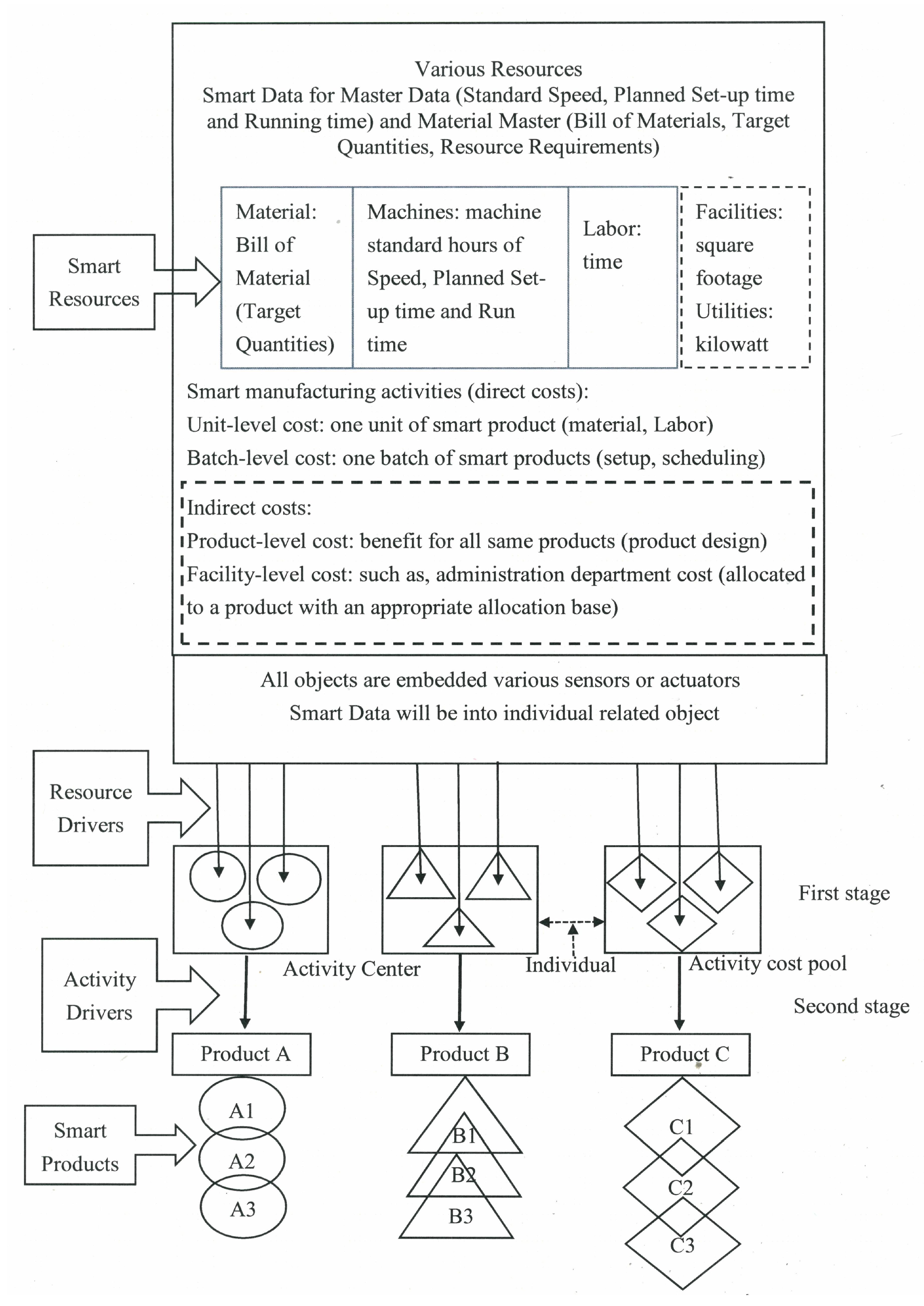
3.3. ABSC in a Smart Factory

The concept of smart products in Industry 4.0 will automatically conduct Activity-Based Standard Costing (ABSC) for real-time information and accurately predict product costs [4,10]. ABSC can recognize different types of activities in a factory, including unit-level, batch-level, product-level, and facility-level activities (e.g., machining a part, setting up a machine, designing a product, and plant management) [38]. Furthermore, creating the smart concept from ABC to ABSC can facilitate setting up the standards of master data and material master lists [24]. First, setting up the related standard measuring of master data includes standard speed, planned set-up, running time, etc. [8,24]. Second, the material master includes bill of materials, target quantities, and resource requirements [14,27]. Finally, the above smart data will be input into the individual related objects in our smart systems before production [45]. All manufacturing objects (e.g., material, machines, products, etc.) are embedded with different sensors to become conscious and intelligent for connecting with each other, and automatically share their information, which will facilitate the prediction and maintenance of machines, control their production processes, and manage the systems in a smart factory [1,7]. Undeniably, in a smart factory, each smart product with embedded sensors can carry its information from resource-components to activity-processes, convey the knowledge of functional guidance for users, track smart products, measure the states of smart products, and analyze the results of smart products [8,10,20].
Regarding the costs of ABSC, an activity center usually clusters the related function and process activities according to their resources. Each type of smart resource will be traced to related activity centers, and become an element of related activity in the cost pools. Various resources and activities assign different ABSC cost to the related products [32]. However, each total cost of an individual specific product can add the costs of related activities, while the same batch or facility costs can be divided by their production quantity for calculating each unit cost [4]. How to calculate accurate costs for each smart product? How to easily achieve the various costs of unit-level, batch-level, product-level, and facility-level in a timely manner for the needs of products, factory, business, and customers [37,38] in a smart factory?

3.4. Standard Costs for Smart Products

In the Industry 4.0 era, strategic cost control must be carried out for all smart products according to the cost assignment view, which includes resources, activities, and cost objects [10,40]. However, the future of smart factories will include cognitive and configuration attributes [20], in order to manage factories, predict and maintain their machines, and control their production processes [1,4,35]. Therefore, all objects in the operation processes are embedded with various smart sensors to become smart objects that can be automated in real-time to connect and exchange information [42]. On the other hand, the strategic costs of all smart objects should be real-time, automatic, and direct, in order to track the activities of each smart product [5].
It is recommended that ABC can achieve the cost accuracy of the product. However, in the Industry 4.0 era, the use of ABSC is necessary to perform real-time accuracy costs for individual smart products. When ABSC is applied to all smart products, each smart product should have a separate strategic cost control. All smart resources can be identified solely by their smart product; thus, their costs should be tracked in a timely, automated, and direct manner [1,4,5].
According to Figure 2, smart data for resources include materials, machines, and labor. First, in the working processes, the direct materials for each product must be controlled with the target quantity of the design bill of material (BOM). Second, before production, the different smart machines for each product must set the relevant standard speed, scheduled setup time, and running time in the relevant machine [1,27]. Finally, the standard direct labor of each product requires planning production management and control according to the time target of standard time, in order to improve labor efficiency during the production process [44]. The resources and activities in this section have different standards (e.g., standard quantities, standard hours). Furthermore, the establishment of the various smart product standards are based on standard quantities (including BOM and standard working hours) and standard unit costs (including direct materials, direct labor, and direct overhead) [8,27].
In particular, various machines will automatically produce many different products, and the machine costs may be a fixed overhead within a period. Therefore, fixed machine costs should be based on the appropriate cost allocation principles, and the fixed costs will be allocated to each smart product [8,44].
However, there are some partial overhead issues, called indirect costs in this research, which come from non-related-manufacturing departments, meaning overhead costs that are not part of the direct standard costs for tracking each smart product. This paper distributes to each smart product by setting an apportion principle of standard costs regarding these indirect costs, such as, the overhead of the administration department or the costs of product-level and facility-level [17,40].
In summary, direct standard material and labor costs for each standard cost of smart products will certainly trace the related resources back to activities of an individual smart product. The direct standard hours of various different smart machines also follow the related model of resource and activity to all smart products, while the machine cost for each smart product should follow the cost of the standard allocation principles [14,25]. Undoubtedly, the indirect standard cost of each standard cost of a smart product is also in line with the distribution principle, and does not track its production process [4,15].

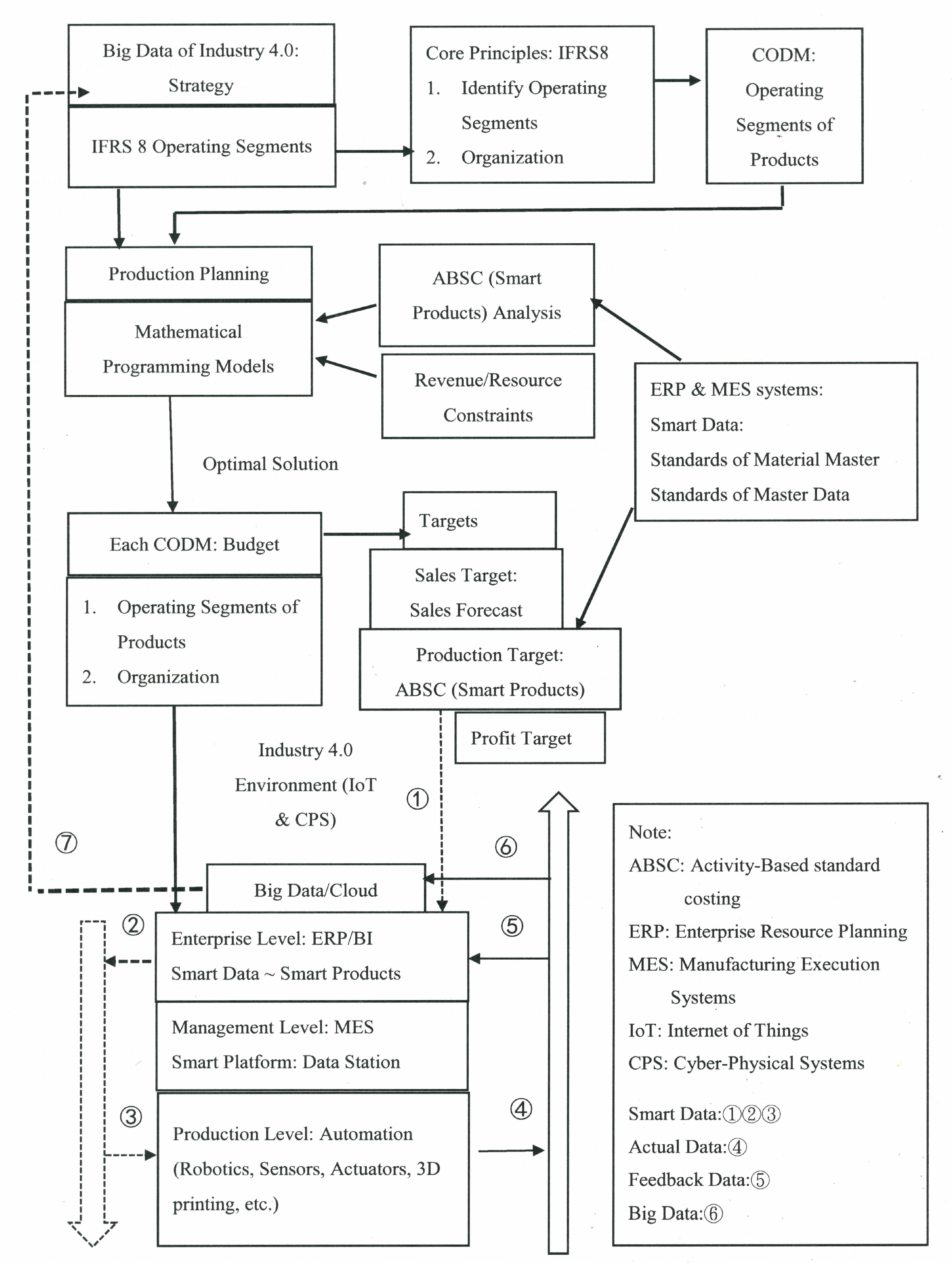
3.5. Production Decision Model of ABSC and IFRS 8 Operating Segments in a Smart Factory

Many companies produce various different products through common or different processes in their factories. Developing a model of Activity-Based Standard Costing (ABSC) according to the ABC model is necessary for the future environment of Industry 4.0. The ABSC model includes: (1) Tracing smart resources (direct resource costs) to related smart activities, (2) allocating indirect costs and providing an appropriate allocation basis for related activities, (3) tracing related activity costs to processes, and (4) tracing the related process costs to final products [4]. The production decision model uses a mathematical programming approach for conducting the important analysis of ABSC real-time information [13,28]. The future ABSC also creates smart individual products with various embedded sensors according to the smart resources of materials, labor, machine hours, etc., in the smart manufacturing processes, and thus create smart products that can be automatically connected end-to-end through the smart Platform of MES in a smart factory [11,37]. This paper integrates various digital smart elements into the ABSC model and the global accounting standards of IFRS 8 to develop an ABSC production decision model that maximizes profits for a public company or a group with a parent company [2,3,28].

4. Formulation of an ABSC Mixed Decision through IFRS 8 for a Steel Group

A variety of optimal models have been designed for production-mix decisions by various mathematical programming methods under ABC [4,32,33,38,40]. The ABSC production decision model can widely use in various factory types. Regarding the systematization and integration of the ABSC production decision model into an international business group, it must be in line with the definitions of the IFRS8 operating segments, and its measurement of reportable segments. Regarding disclosing the revenue of IFRS 8, the reported revenues include external customers, intersegment sales and transfers [16]. Consolidated financial statements include revenues and expenses for the business activities of the same operating segment [2,3]. In the digital age, the extended ABSC model is based on ABC, smart data and real-time information [4,8]. Figure 3 compares ABC and ABSC.

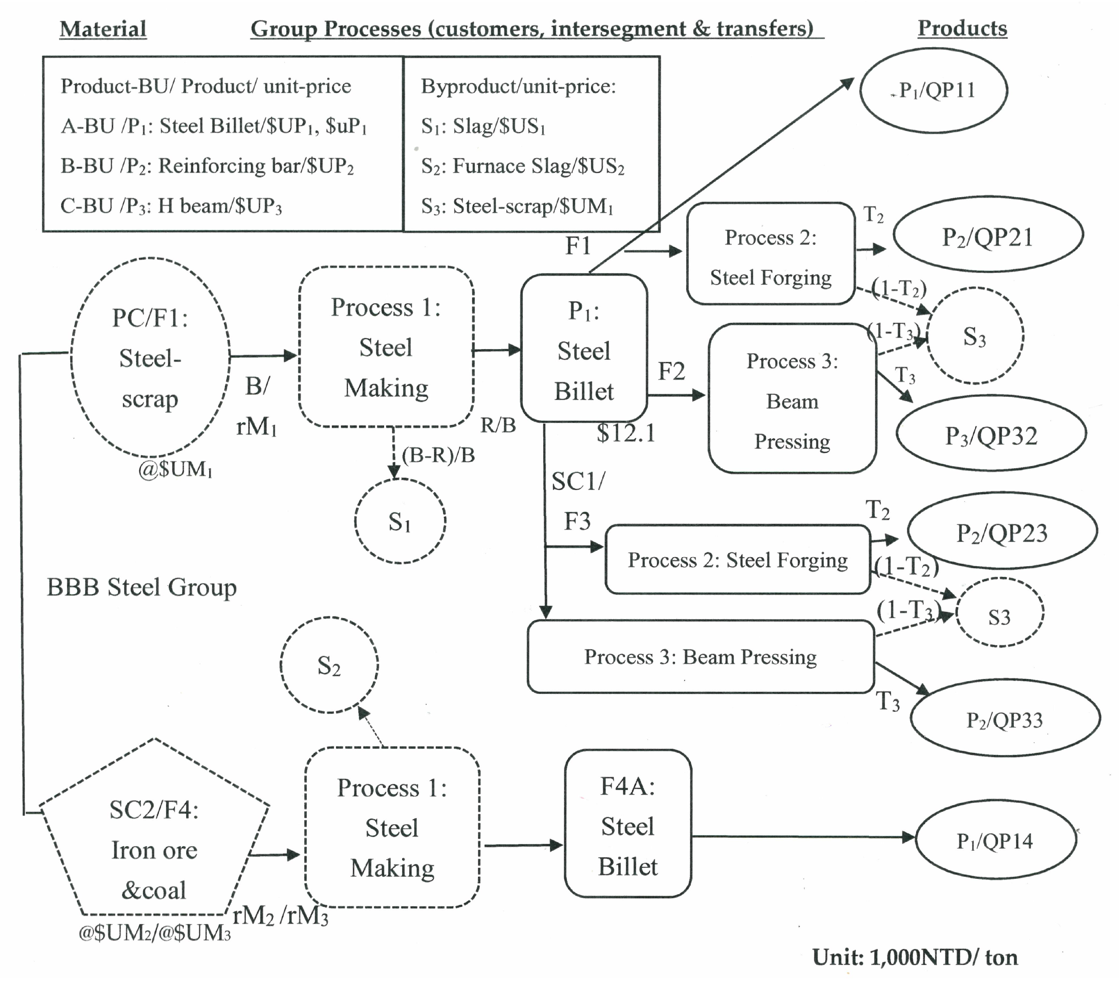
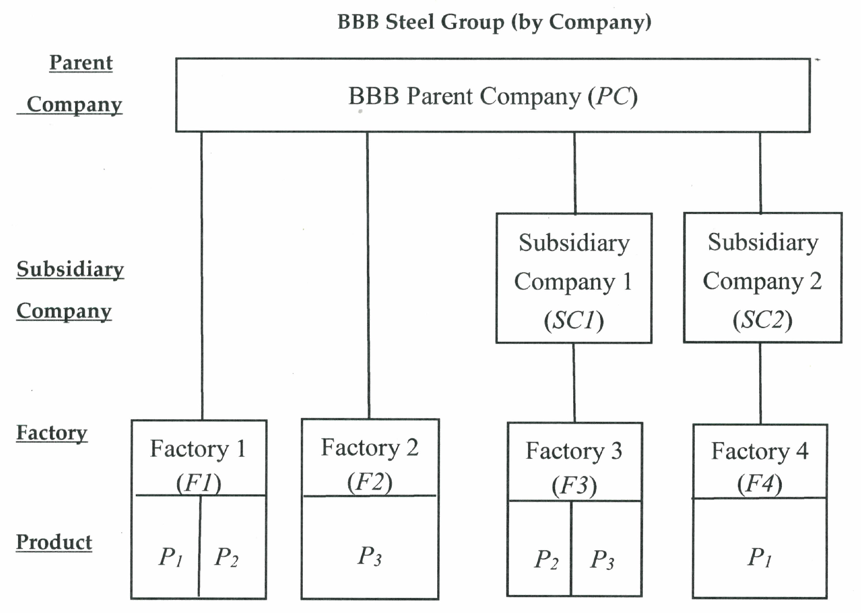
4.1. Describing Production Processes for a Steel Group

Figure 4 shows a description of the manufacturing processes for an international steel group. This study includes various discussions: Firstly, designing and following the IFRS 8 operating segments plan regarding the manufacturing relationship of all factories and processes in a steel group [3,46]. Secondly, following the revenue’s definition of IFRS 8 standards, the revenue of a business group includes external customers, the intersegment sales of different company, and transfers of the same company [3]. Thirdly, comparing process 1 in steel making, different materials and manufacturing methods have different cost elements and output. Lastly, three different kinds of byproducts are output in different processes.

4.2. Steel Group Cost Categories for the ABSC Mixed Decision Model

The planed result of the profit target is from the sales target to the production target (including all standard costs) [44], as shown the middle part of Figure 1. Firstly, the design of product-based organization for a steel group, which defines each operating segment and will be the basis for separating its financial statements [3,6]. We also call Product-BU (Product-Business Unit) as each operating segment. Secondly, following IFRS 8 standards, the CODM of each entity must review all its Product-BUs from sales targets to profit targets. Lastly, in the smart data design for ERP and MES systems, all targets for sales, production, and profit must be separated by the relevant Product-BU [3,36]. This study classifies revenue and six costs categories, as follows:
  • Revenue: Including sales products, byproducts, intersegment sales (selling P1 to other relational companies in the same group), and the transfer of internal products (transfer of P1 to the same company for B-BU or C-BU);
  • Material costs: Including steel scrap for EAF (Electric Arc Furnace) manufacturing, and Iron ore and coal for BF (Blast Furnace) traditional manufacturing;
  • Labor cost: Including normal and overtime direct labor cost, and indirect labor cost for EAF;
  • Electrical power cost: Only suitable for high electrical power cost in the steelmaking process by using EAF equipment. Electricity bills for other processes are not important, so their electrical power costs are included in other costs.
  • CO2 emission cost: Including carbon tax and carbon right costs;
  • Machine costs: Allocating and installing all machines with smart data in the related working process; however, the machine cost is fixed;
  • Other costs: Other indirect costs using only the percentage of revenue-customer;
The flowchart in Figure 4 describes a steel group’s processes from material to products (the quantities of each product equal the sales forecast). The study integrates all resources and production processes of the steel group to maximize profits. Adapting the mathematical programming method will achieve optimal decision-making by using a LINGO system [4,33]. This study contributes a group of multiple Product-BUs organization [2,3], which not only follows IFRS 8 standards, it also extends the ABSC model of a group, which will achieve smart manufacturing through various systems, ERP and MES systems [4,37].

4.3. Assumptions

The Product-BU organization of a steel group follows the IFRS 8 standards in all production processes of the group [2,3,11]. Supposing the group takes the ABSC production decision, all production operations from a variety of revenue to costs are integrated into several assumptions and mathematical programming models [28,36], as follows;
  • Following the IFRS 8 standards [3], total revenue including: External sales, semi-manufactured goods of P1 (for selling different BU, including the same company or related company in the same group), and byproducts (for selling slag or furnace slag);
  • Different direct raw materials are used in different manufacturing methods; and the recycling byproduct of steel scrap also become its direct material;
  • Direct labor will be relevant to manufacturing methods, production processes, and machine hours;
  • Conforming to government policies, including basic wage, overtime hours, carbon tax, and carbon right costs;
  • Direct costs, including: Raw material, labor, electrical power cost, and CO2 emission;
  • Smart machines will run automatically by being embedded into various smart data, while the machine cost is fixed;
  • Indirect costs are not related to the production processes, but all smart products must share the costs at a fixed percentage of external sales.

4.4. Notations

The following descriptions of codes are used for this paper as shown in Table 1 for Organization Related Codes and Table 2 for ABSC Related Codes.

4.5. Mathematical Programming Model

According to this section, this case follows the IFRS 8 standards and formulates the categories of revenues and costs for the ABSC mixed decision model [20]. Firstly, this case has three revenue categories, including external sales, transfers, and intersegment sales. Additionally, P1 semi-manufactured product is sold from A-BU to B-BU or C-BU, and produce P2 or P3, respectively, in the same or different factories/companies, but in the same group. Secondly, this group has six cost categories, including direct material cost, direct labor cost, fixed smart machine cost, electrical power cost, CO2 emission cost, and indirect cost. Those categories of revenues and costs will be incorporated into a mathematical programming model. The following describes the status of related sales and costs, and discusses them with a model. Planning a mathematical programming model and ABSC production decision model will obtain the optimal solutions in the future [4,33]. Furthermore, each Product-BU has prepared a number of consolidated financial statements for the reportable segment through all its information in the ERP system, and CODM will review these statements each accounting period [3].

4.5.1. Integrated Models

Maximize total profit Ω :
Ω = [ ( p = 1 3 Q P p U P p ) + ( q P 1 u P 1 ) + ( b = 1 2 Q S b U S b ) ] [ ( m = 1 3 Q M m U M m ) ( Q S 3 U M 1 ) { C L s + [ C L 1 + δ 1 ( C L 2 C L 1 ) + δ 2 ( C L 3 C L 1 ) ] + C L v } ( E d X U E ) ( f = 1 4 C I f ] [ π 1 U Z 1 ( W 1 Q Z 1 ) + π 2 U Z 2 ( W 2 Q Z 1 ) ] ( f = 1 4 C G f )
Subject to:
A1. Products for customers constraints:
QM1 = (QP11 + qP1) + QS1;
QP2 = QP21 + QP23;
QP3 = QP32 + QP33;
A2. Products for the intersegment sales and transfers constraints:
qP1 = (QP111 + QP112 + QP113); qP1 = (QP2 * T2) + (QP3 * T3); QP1 = QP11 + QP14;
A3. Byproducts constraints:
QS1 = QM1 − (QP11 + qP1); QS2 = QP14 * 0.5; QS3 = qP1 − (QP2 + QP3);
B1. Direct material quantity constraints:
QM1 = B * X; QM1 = rM1 * (QP11 + qP1); QM2 = rM2 * QP14; QM3 = rM2 * QP14;
C. Direct labor hour constraints:
H = H1 + δ1 (H2 − H1)+δ2 (H3 − H1); H1 = (NL * αh1); (H2 − H1) = NL * αh2; H3 − H2 = (NL * αh3)
QP2 * Bh+ QP3 * Ch = H1 + δ1(H2 − H1) + δ2(H3 − H1);
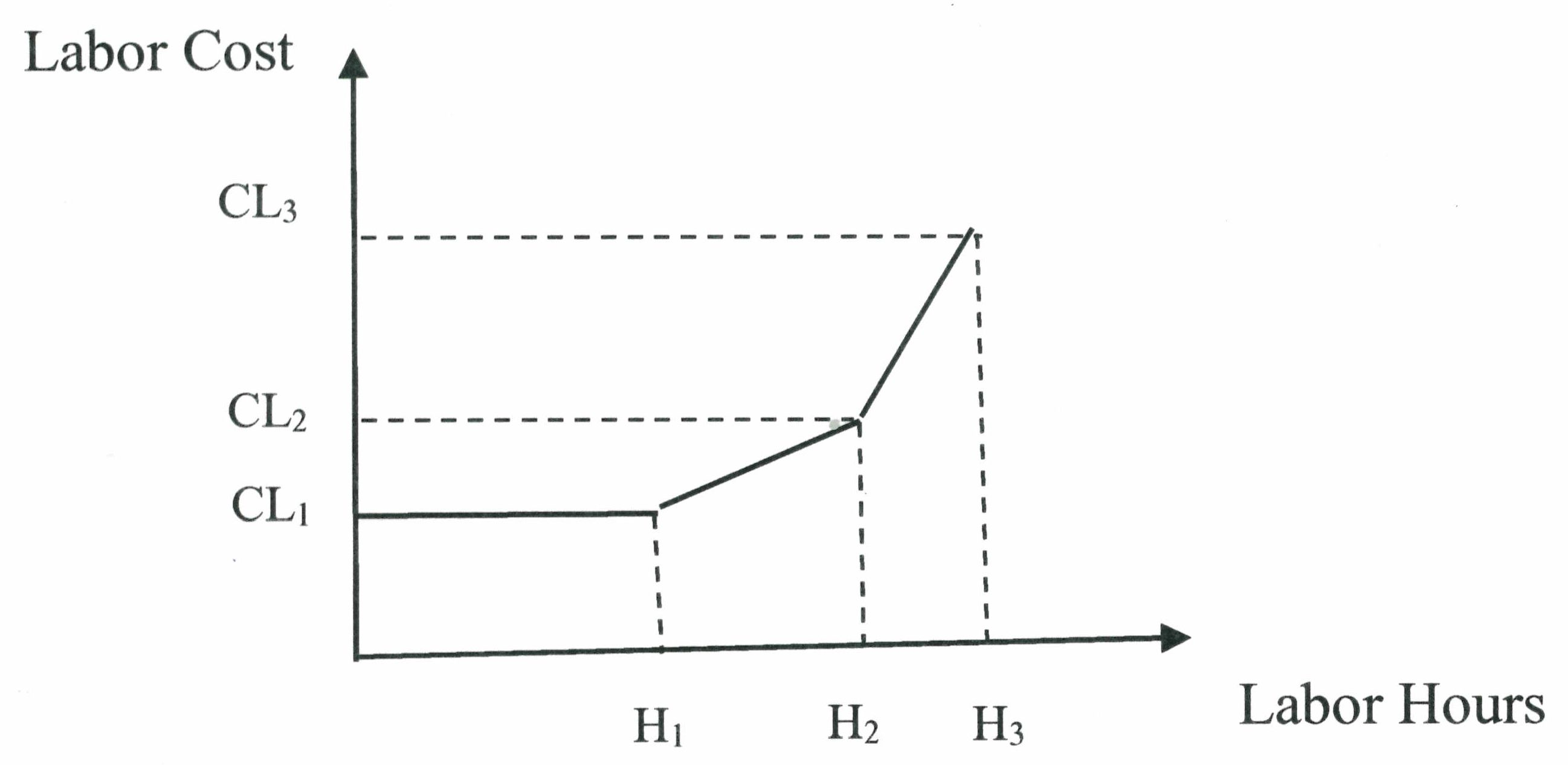
(H2 − H1) ≤ 22 * (NL1 + NL2 + NL3); (H3 − H1) ≤ 40 * (NL1 + NL2 + NL3);
δ0 − ε1 ≤ 0,
δ1 − ε1 − ε2 ≤ 0,
δ2 − ε2 ≤ 0,
δ012 = 1 0 ≤ δ0, δ1, δ2 ≤ 1
ε1 + ε2 = 1 ε12 = 0, 1,
D. Machine hour constraints:
Ih0 = X * Ab; Ih1 = QP14 * Ah; Ih2 = QP2 * Bh;; Ih3 = QP3 * Ch;
E. CO2 emission constraints:
( Q P 1 R Z f ) = E Q f
EQf = Wf0 + Wf1 + Wf2
0     W f 0     QZ 1     π 0 ,  
QZ 1     π 1   <   W f 1     QZ 2   π 1 ,  
W f 2   >   QZ 2   π 2 ,
π 0 + π 1 + π 2 = 1 ,   π 0 , π 1 , π 2 = 0 , 1 .

4.5.2. Sales Amount Following IFRS 8 Standards

According to Figure 4 and IFRS 8 standards, the revenues include external customers, intersegment sales and transfers [3,28], and byproducts. The BBB group has three products: Steel billet (P1), steel reinforcing bars (P2), and H beams (P3), and the sales unit prices (UPp) are (UP1), (UP2), and (UP3), respectively. On the other hand, the internal P1 sales unit price is (uP1) for intersegment sales or transfers in the group. Additionally, the salable byproducts apply only to slag (S1) and furnace slag (S2).
First, the BBB group has three Product-BUs for three products, and includes P1-steel billets (A-BU), P2-steel reinforcing bars (B-BU), and P3-H beams (C-BU). Producing all products will be properly arranged in the group’s different processes/factories/companies for production. P1 products can be sold to customers or regarded as semi-manufactured goods for continuously manufacturing P2 or P3 products. The total customer sales amount is Equation (1), i.e.: p = 1 3 QP p UP p .
Secondly, selling the intersegment sales and transfers in the group, is only the P1 product. The production of P1 is in the factory (F1) at the Parent Company (PC). Most P1 production is for the continuous production of P2 or P3 products in different process/factory/company, such as, intersegment sales to Factory 3 (F3) of Subsidiary Company 1 (SC1) and intersegment transfers to F1 or F2. Thus, the total P1 intersegment sales and transfers are for B-BU or C-BU by Equations (1), i.e.: (qP1 * uP1).
Lastly, in the different processes, three byproducts are produced by all production processes, including: S1-slag, S2-furnace slag, and S3-steel scrap. Salable byproducts are available only for S1 and S2, in quantities of QS1 and QS2, and with unit prices of US1 and US2. Thus, the total amount of Byproducts is as Equation (1), i.e.: ( b = 1 2 QS b US b ) .
In summary, the total revenue comes from external sales, intersegment sales, transfers, and byproducts; in Equation (1), i.e.:   ( p = 1 3 U P p Q P p ) + ( u P 1 q P 1 ) + ( b = 1 2 U S b Q S b ) . This paper also considers some constraints on the number of sales of external customers and internal groups, as in Equations (2)–(4).

4.5.3. Direct Material Cost

The terms in Equation (1), i.e.: [ ( m = 1 3 QM m UM m ) ( QS 3 UM 1 ) ]   expresses the total direct material cost of purchasing steel scrap (M1), Iron ore (M2), and coal (M3), and recycling the byproduct of steel scrap (S3). Firstly, in Factory 1 (F1) steel making process using batch-level production, the raw material of steel scrap (M1) will be poured into advanced EAF manufacturing, where each batch of weight is B, and each batch of production P1 quantity is R. Assume that the standard M1 requirement is rM1 and it equals B/R for one unit of steel billet (P1). In an accounting period, the number of batch is X. Therefore, the quantity of steel scrap (QM1) equals B * X. The unit cost of steel scrap is UM1. Thus, the total material cost of steel scrap (CM1) equals (QM1) * (UM1). Secondly, in Factory 4 (F4) steel making process using unit-level, it is a continuous manufacturing process using the BF method. The direct materials for BF are iron ore (M2) and coal (M3). For one P1 unit, the standard requirements for Iron ore and Coal are rM2 and rM3, respectively. The quantity of Iron ore (QM2) is equal to QP4 * rM2 and the quantity of Coal (QM3) is equal to QP4 * rM3 in a period. The total material costs of M2 and M3 are QM2 * UM2 and QM3 * UM3, respectively. Lastly, the unit price of the recycling byproduct of steel scrap (S3) is same as that of UM1, meaning the S3 byproduct comes from the steel forging and beam pressing processes in Factories 1–3. The quantity of S3 is QS3, and the recycling material cost is QS3 * UM1. To sum up, the direct material cost is as Equation (1) i.e.: [ ( m = 1 3 QM m UM m ) - ( QS 3 UM 1 ) ] . We also consider some constraints of material quantity for producing P1 by using EAF or BF for customers or internal groups, as in Equation (5).

4.5.4. Semi-Manufactured Goods

The steel forging and beam pressing processes are continuous production processes with input material from the semi-manufactured goods of P1. Assuming that the bill of materials for P2 and P3 are P1 semi-manufactured goods, and P2 or P3 standard requirements apply to T2 and T3, respectively. In Equation (3), we consider some constraints in the production of P1 semi-manufactured goods for P2 and P3.

4.5.5. Direct Labor Cost

Figure 5 shows a piecewise linear graph that represents (1) the basic hours of direct labor at H1, (2) overtime at H2, and (3) holiday overtime at H3; and the direct labor costs arrive at CL1, CL2 and CL3, respectively. First, in an accounting period, the basic direct hours and minimum wage are at H1 and CL1 including the number of direct labor (NL) * working hours per labor (αh1) one period and the number of direct labors (NL) * the basic wage each labor (α); in other words, H1 equals (NL * αh1) and CL1 equals (NL * α). Second, the overtime hours and the wage equal the number of direct labors (NL) * the overtime hour per labor (αh2) and the number of direct labors (NL) * (αh2) * the overtime wage each hour (θ2), as (NL * αh2 = H2 − H1) and (NL * αh2 * θ2 = CL2 − CL1). Last, the holiday-overtime hours and the wage equal the number of direct labors (NL) * the holiday-overtime hour per labor (αh3) and the number of direct labors (NL) * (αh3) * the overtime wage each hour (θ3), as (NL * αh3 = H3 − H2) and (NL * αh3 * θ3 = CL3 − CL2). However, the results of total hours (basic + overtime + holiday overtime) are presented in Equation (6): H = H1 + δ1(H2 − H1) + δ2(H3 − H1). On the other hand, we present the piecewise direct labor cost in Equation (1), i.e.: CL1 + δ1(CL2 − CL1) + δ2(CL3 − CL1). As shown in Figure 5.
According to Equation (6), the total labor hours are composed of three parts with basic, overtime, and holiday overtime hours. Where (ε1, ε2) in Equation (12) is a SOS1 set of 0–1 variables, within which certainly one variable must be non-zero;( δ0, δ1, δ2) in Equation (11) is a SOS2 set of non-negative variables, within which at the most two adjacent, in the order given to the set, can be non-zero (Williams 1985). In Equation (6)–(12), if ε2 = 1, then ε1 = 0 in Equation (12), δ0 = 0, δ1,δ2     1, and δ1 + δ2 = 1 in Equation (11). Thus, the total labor hours are H1 + δ1(H2 − H1) + δ2(H3 − H1) in Equation (6), and the total labor costs are CL1 + δ1(CL2 − CL1) + δ2(CL3 − CL1) in Equation (1). We also consider some constraints for working time, overtime, holiday overtime, and standard hours for P2 and P3, in Equations (6)–(12).

4.5.6. Other Fixed Labor Costs

Advanced EAF in the steel making process must use special indirect labor to operate the related special equipment. The number of indirect labor is NIL. All special indirect laborers only work on normal working days, and their salaries are twice the times higher than direct labor; thus, the indirect labor cost is fixed and equals CLs = NIL * 2α. On the other hand, the traditional Blast Furnace (BF) in the steel making process does not interrupt continuous production operations. All direct laborers must be operated in three shifts; thus, its labor cost is also fixed (including fixed salary and holiday overtime).

4.5.7. Direct Electricity Power Cost

In this subsection, advanced EAF with high electric power consumption for the production of P1 in the steel making process. The terms in Equation (1), i.e.: Ed * X * UE. The cost of electricity power is calculated in batches. We assume that each batch requires the electric degree of Ed, the total number of batches is X, and the unit cost is UE; thus, the total cost is CE = Ed * X * UE.

4.5.8. Machine Cost

The machines used in each process are different; however, the machine costs are fixed for each process, regardless of machine usage time. The terms in Equation (1), i.e.: f = 1 4 CI f   represents the machine cost per factory. However, in Equation (13), the machine hours will consider some constraints of batch-level and unit-level in each process.

4.5.9. CO2 Emission Cost

For the carbon tax cost function, the terms in Equation (1), [π1 * (Wf1 − QZ1) * UZ1 + π2 * (Wf2 − QZ1) * UZ2] .   In Figure 6, the associated quantity constraints are expressed in Equations (14)–(19). In Equation (14), the total carbon quantity is EQf = Wf0 + Wf1 + Wf2. There are three carbon tax costs depending on the quantity of EQf. First, the tax cost is free (π0 = 1, π1 = 0, π2 = 0) if the quantity of EQf is less than QZ1. Second, the carbon unit cost is UZ1 (only π1 = 1) and the total cost is (Wf1 − QZ1) * UZ1, if the EQf is more than QZ1 and EQf is less the QZ2 (Wf1 = QZ2 − QZ1). Last, the carbon unit cost is UZ2 (only π = 1) and the total cost is (Wf2 − QZ1) * UZ2, if the EQf is more than QZ2. However, producing P1 by using EAF or BF will result in different quantities of CO2 emissions.

4.5.10. Other Indirect Costs

The terms in the last set of parentheses in Equation (1), i.e.: f = 1 4 CG f uses each product only as the rp percentage of customer revenue to represent the total amount of other indirect costs.

5. Illustrative Case Study

This section presents a numerical example and discusses the application of the ABSC production decision model of a steel group. We follow the smart operating roadmap, as shown in Figure 1, meaning how an international group strategizes to plan and execute. Firstly, according to the IFRS 8 operating segments, the strategic models of the BBB group company and BU group organization in the ERP system is designed, and the operation process of group organization is also embedded [2,3,7]. Secondly, the planning approach includes smart data, sales forecast, ABSC analysis, various revenue and resource constraints, etc., which will be discussed and itemized [13,36]. Finally, this study designs an individual management report of reportable segments for the BBB group, which divides each company into different BU segments.

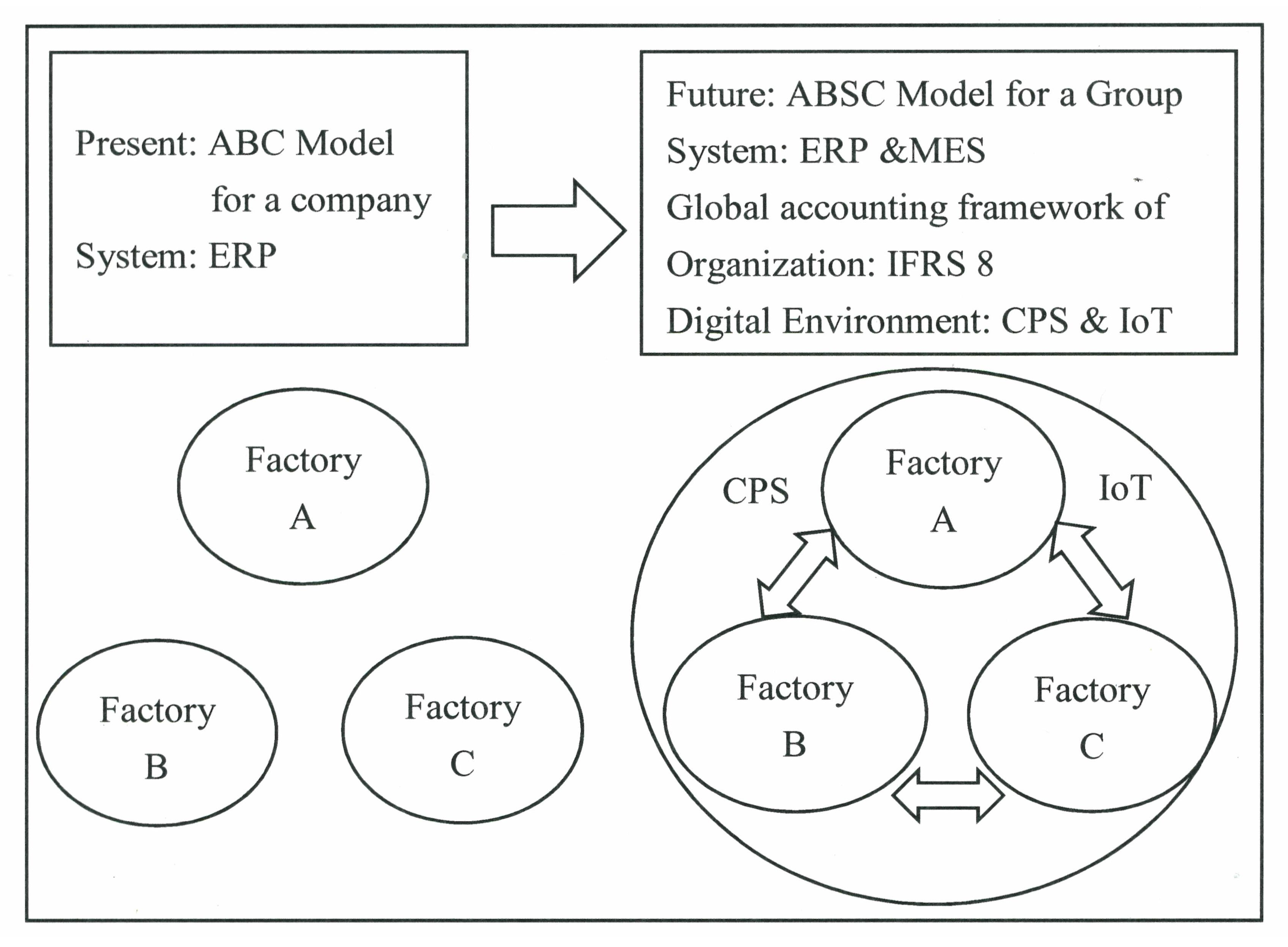
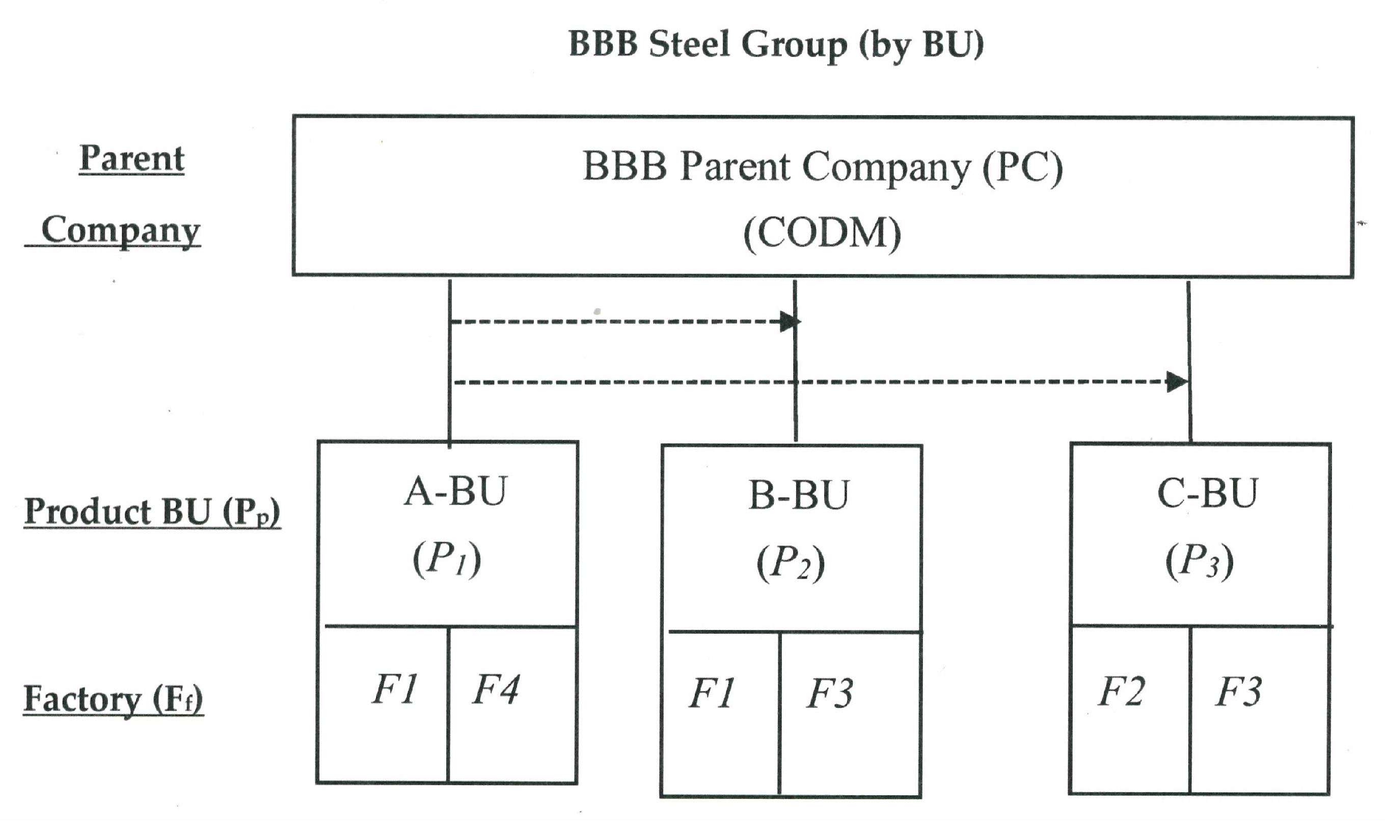
5.1. Strategy Model for Group Organization

According to the two core principles in Figure 1, we identify the product-operating segments and formulate the two different organizations of a company group and a BU group, as shown in Figure 7 and Figure 8, respectively. In a BBB steel group, assume that its Parent Company (PC) is a public company in Taiwan, and is required to comply with IFRS standards. From an organizational point of view, the Parent Company (PC) has two subsidiaries (SC1 and SC2) and four factories (F1, F2, F3 and F4), meaning a company group organization, as shown in Figure 7. The group has three products, including P1, P2 and P3 and applies BU group organization [3,11], as shown in Figure 8.

Smart Data and Sales Forecast

In the Industry 4.0 era, smart data are an important issue for setting up all related standards of master data and material master into our smart systems before production [8,43]. Regarding the identification of operating segments and measurement of reportable segments, the company-code and factory-code must be interconnected through all process/activity centers for collecting all real-time information during all operating processes [7,10,25]
Following the notations in Section 4.4, we arranged some notations of organization and sales forecast, which became our smart data (Table 3), which are stored in a smart ERP system before production [36]. The smart data also can be obtained through MES’s data station and installed into related smart machines or smart robots [19].
However, the sales forecast also considers the quantity of each product in the group’s operating policies, which is due to market constraints, the needs of the BBB internal group transfers, and intersegment sales.
Firstly, in Table 3, P1 products are produced in the first factory (F1) or fourth factory (F4). (1) P1 productions from the F1 are sold to customers (QP11), as well as transferred to the steel forging’s process (QP111) for the production of P2 products (QP21). (2) Then, P1 products are transferred (QP112) from F1 to F2, which is a different factory (F2), to produce P3 products (QP32). (3) The F1’s P1 products are sold to the intersegment (QP113) of the same group, but a different SC1 company to produce P2 (QP23) and P3 (QP33) products. (4) In F4, the production of P1 products is used only for sales customers (QP14).
Secondly, following the above, P1 products are semi-manufactured goods, which are continuously produced in the steel forging and beam pressing processes, and produce P2 and P3 products in Factories 1–3, including the same factory (F1), the same “PC” company (F2), the same “BBB” group (F3). In the IFRS 8 operating segments, the reported revenues must include external customers, intersegment sales, and transfers [3]. Therefore, in this case, P1 semi-manufacturing goods belong to the internal BBB group’s intersegment sales (F3 of “SC1” company) and the transfer revenue (F1 and F2 of “PC” company).
Finally, the quantitative constraints of the above sales and semi-manufactured goods include (1) QP11, QP14, QP21, and QP33, which are less than, 10,000, 36,000, 17,600, and 19,300, respectively; (2) QP23 is between 14,000 and 17,200, and, QP32 is between 22,000 and 24,000; which is due to the limitations of each factory.

5.2. Process Planning

This BBB steel group case is based on Figure 4. We will present an example that includes all production processes of different companies/factories to maximize profit [47]. Assume that the BBB group has three Business Units (BUs) for the production of different products for P1, P2 and P3. Specially, P1 in the F1 or F4 steel making process; however, their production technologies are different. In F1, modern EAF technology adapts steel scrap recycling materials, which not only saves many traditional mining, dressing, coking, and ironmaking manufacturing processes, it also saves mass natural resources and energy. In F4, the traditional technology of a Blast Furnace (BF) produces high pollution during its manufacturing process. While they can produce the same P1 product, the production models of EAF and BF are completely different in all operations, from raw material input to byproduct output [46,47]. On the other hand, P1 is not only a finished product for external customers; it is also semi-manufactured goods for intersegment sales or transfers in the group. The following describes more various costs for this group.

5.3. Direct Material and Semi-Manufactured Goods

The terms in Equation (1), i.e.: [( m = 1 3 QMm UMm ) − (QS3 * UM1)], it expresses the total direct material cost, (1) the purchase of steel scrap (M1) for the EAF manufacturing method, (2) the purchase of Iron ore (M2) and coal (M3) for the BF manufacturing method, and (3) QS3 byproducts are produced during the production of P2 and P3. According to the smart data for the standard material master is the Bill of Materials (BOM).
Firstly, regarding the batch-level of EAF in Factory 1(F1), the steel scrap of each batch of direct material (M1) is 100 tons, the notation is (B), the output of P1 is R (90 tons), and the byproduct quantity is (B-R) per batch. The total number of batches is X in an accounting period. We assume that the bill of materials for the P1 unit is a standard requirement for steel scrap (M1) and rM1 (100/90 = 1.11 tons). The unit price of steel scrap is UM1. In other words, the demand for steel scrap (QM1) equals B * X, and QM1 equals rM1 * (QP11 + qP1), which is the quantities of sales forecast in Table 3. The total material cost of steel scrap is (QM1 * UM1) in a period.
Secondly, regarding the unit-level of BF in Factory 4 (F4), assuming that one unit of P1 is the standard requirements for Iron ore and Coal are rM2 (2.9 tons) and rM3 (0.9 tons), with the unit prices of UM2 and UM3, respectively. The demand for Iron ore (QM2) is equal to QP14 * rM2 and another demand for Coal (QM3) is equal to QP4 * rM3. The total material costs of M2 and M3 are UM2 * QM2 and UM3 * QM3, respectively. On the other hand, assume that the byproduct quantity (QS2) equals 0.5 * QP14.
Lastly, the unit price of steel scrap byproduct (S3) is same as the unit price of steel scrap procurement materials (UM1). Steel scrap byproduct (S3) output comes from steel forging and beam pressing processes for the production of P2 or P3. The standard material master (such as BOM) [8] is the P1 semi-manufactured goods that produces P2 (T2 = 1.02) and P3 (T3 = 1.03) products. According to the quantities of sales forecast for products (P2 and P3), the total quantity of byproduct (QS3) equals {[(QP2 * T2) + (QP3 * T3)] − (QP2 + QP3)}. The total recycling material cost of S3 is QS3 * UM1. In this case, the unit purchasing costs of direct material (UMm) include UM1 = NTD9100, UM2 = NTD3200 and UM3 = NTD2200. On the other hand, the direct material quantity constraints are QM1, QM2, QM3 less than 95000 (X950), 100,000 and 50,000, respectively. To sum up, the direct material cost is in Equation (1) i.e.: [( m = 1 3 Q M m U m m )-( QS3 * UM1)].

5.4. Direct Labor for Unit-Level

Direct laborers are used in Factories 1–3 (F1, F2, F3) in Taiwan and Factory 4 (F4) in Vietnam. The total number of direct labor is 1000 (NL) workers in the BBB group, including F1 (NL1 = 150), F2 (NL2 = 250), F3 (NL3 = 300) and F4 (NL4 = 300). Accord to the Basic Wage Committee in Taiwan, the monthly minimum wage and working hours for each direct labor are α (NTD26,400) and αh (176 h, including 22 working days and 8 h per working day). Wage rates include normal hourly rate (θ1 = NTD150), overtime (θ2 = NTD225), and holiday overtime (θ3 = NTD300). Another, which follows the reportable segment of IFRS 8 standards [48], and in the same currency, assumes that the monthly minimum wage and working hours in Vietnam are β (NTD6000 = VND4,539,000) and that the exchange rate is 1NTD = 756.5 VND and βh (200 h) for each direct laborer [19,25]. The Vietnamese wage rate for each direct laborer includes normal hourly (λ1 = NTD30), overtime (λ2 = NTD45), holiday overtime (λ3 = NTD60).
According to the smart data of the master data (for example, standard speed, planned set-up time, and run time) using unit-level direct labor, we assume that Taiwan’s standard operating time is P2 per ton of Bh (1.5 h) and P3 per ton of Ch (2 h). In the factory in Vietnam (F4), the standard operating time for P1 product is Ah (2 h). At factories 1–3 (F1, F2, F3) in Taiwan, each worker does not exceed 40 h per month to limit overtime, and each worker can only work 9 h a working day. At factory 4 (F4) in Vietnam, it is a 24-h continuous manufacturing factory; thus, it has to do three shifts of direct uninterrupted labor production. Its monthly working days is 30 days including 25 normal days ( β d )   and 5 days of holiday overtime. As a result, its wage rates are only normal hourly wages (λ1 = NTD30) and hourly overtime (λ3 = NTD60).
To sum up, Figure 5 shows the piecewise linear results that only apply to P2 and P3 in Factories 1–3 (F1, F2, F3). In terms of total direct labor hours in Factories 1–3, H1 denotes (NL1 + NL2 + NL3) * 176 labor hours at basic wage rate of NTD150 (θ1) per hour, while H2 denotes H1 + (NL1 + NL2 + NL3) * 22 labor hours at the overtime wage rate of NTD225 (θ2) per hour, and H2 denotes H2 + (NL1 + NL2 + NL3) * (40 − 22) labor hours at the holiday overtime wage rate of NTD300 (θ3) per hour. However, in accordance with IFRS 8, each product in each factory should have its own individual financial statements [38]. Therefore, the total labor hours are H = H1 + δ1(H2 − H1) + δ2(H3 − H1) in Section 4.5.5 should be separated F1 (QP21 * 1.5 ≤ NL1 * 176), F2 (QP32 * 2 = 44,000 + r21 * (49,500 − 44,000) + r22 * (54,000 − 44,000)) and F3((QP23 * 1.5) + (QP33 * 2) = 52800 + r31 * (59,400 − 52,800) + r32 * (64,800 − 52,800)). Another, the total labor costs (unit = NTD1000) are CL1 + δ1(CL2 − CL1) + δ2(CL3 − CL1) also should be separated F1(3960), F2(6600 + r21 * (7837.5 − 6600) + r22 * (9187.5 − 6600)) and F3(7920 + r31 * (9405 − 7920) + r32 * (11025 − 7920)). The F4 in Vietnam has to continuously produce P1 by adapting three shifts of direct labor for whole day production; thus, its direct labor is a fix labor cost each month. Its direct labor cost equals CLv = (NL4 * β) + (NL4 * 5 * 8 * λ3) = NTD2,520,000.

Indirect Labor for Batch-Level

We assume that there are 70 (NIL) indirect laborers engaged in the steel making process using EAF to produce the P1 product in Factory 1 (F1). All special indirect laborers work only on normal working days, 8 hours per working day, and 22 working days in a period. On the other hand, all indirect labor wages are twice the direct wage. Therefore, the wage of indirect labor is a fixed cost (CLs), the cost is equal to CLs = NIL * 2α = NTD 3,696,000 in each period.

5.5. Electricity Power Cost only for EAF

This subsection is the cost of electricity power. Each batch of 100 tons (B) of steel scrap is poured into an EAF. The total number of batches is X. The production time per batch is 0.75 h and requires 45-kilowatt(Ed). The unit cost of UE is NTD2600. Thus, the total cost is CE, which is equal to Ed * X * UE in Equation (1).

5.6. Machine Hours and Cost

Depending on the machine hours of master data for smart data (for example: Set-up time and run time) [49] for the unit-level of machine hours, we assume that the standard operating times for Taiwan factories (F1, F2, F3) are Bh (1.5 h) per ton of P2, and Ch (2 h) per ton of P3. In the Vietnam factory (F4), the standard operating time for P1 is Ah (2 h). The standard machine hours of P1, P2 and P3 are the same as the labor hours including Ah, Bh and Ch, respectively. According to the sales forecast in Table 3, the machine hours for QP14, QP2 and QP3 are Ah * QP14, Bh * QP2 and Ch * QP3, respectively. On the other hand, the EAF process is a batch process with a running time of 0.75 h, which is the same as each batch of electricity power time. In each process of machine cost, both unit-level and batch-level are fixed cost. The machine costs of F1–4 are NTD45,000,000, NTD4,500,000, NTD6,5000,000 and NTD8,500,000, respectively. Therefore, the total machine cost is NTD 64,500,000 in Equation (1) i.e.: f = 1 4 CI f .
However, according to IFRS 8 operating segments, different operating segments must have their own individual financial statements in the same company [3]. Therefore, the machine costs of F1 and F3 should be distinguished from different products, including NTD42,000,000 of P1 (for seven EAFs) and NTD3,000,000 of P2 in F1, and NTD3,000,000 of P2 and NTD3,500,000 of P3 in F3.

5.7. CO2 Emission Quantity and Cost

This part is for CO2 emission quantity and cost. The steel making process for producing P1 can use the EAF in Factory 1(F1) or BF in Factory 4 (F4), and compared with the traditional BF technology and modern EAF technology, carbon pollution is significantly reduced by 75%. Assuming that the production of P1 and the use of EAF will produce CO2 emissions of 40% (RZ1), and another P1 product using BF will produce CO2 emissions of 160% (RZ2) [4]. In this case, according to the sales forecast in Table 3, the quantities of CO2 emission of EAF and BF are [(QP11 + QP111 + QP112 + QP113) * 40%] and (QP14 * 160%), respectively. The carbon tax cost function is (π1 * UZ1 * (Wf1-QZ1) + π2 * UZ2 * (Wf2 –QZ1)), as shown in Equation (1). Assume that the quantity (EQf) of CO2 emission is less than 5000 (QZ1) tons and has a free carbon tax rate (π0 = 1, π1 = 0, π2 = 0); the unit cost is UZ1 (NTD60/each ton, only π = 1) when EQf is between 5000 tons (QZ1) and 10,000 tons (QZ2); the highest unit cost is UZ2 (NTD90/each ton, only π2 = 1) when EQf is more than 10,000 tons.
In particular, in line with the government’s policy of rewarding the greening of the production process, from a CSR report of a public steel company [46], the production process of EAF can reduce CO2 emissions and use recycled materials to produce the P1 steel billet product to improve and protect our environment. In this case for Factory 1 (F1), it is assumed that government incentives can reduce the cost of NTD2,100,000 (for seven EAFs) CO2 emissions per period.

5.8. Other Indirect Costs

The last part is for other indirect costs using the rp percentage of the Pp product’s customer revenue from different factories, as shown in Equation (1); i.e.: f = 1 4 CG f . Other indirect costs are complex costs that can hardly be explained in detail (for example, costs at the product-level and facility-level, and overhead costs for the administration department). However, following compliance with IFRS 8, different BUs must have its own individual financial statements in the same company [3]. Therefore, the other indirect costs of each kind of product in the same factory should be distinguished. Assume that the percentages of rp include 3%, 5% and 5% of P1, P2, and P3 products, respectively, and the sales quantities are estimated as the sales forecast (Table 3), such as QP11, QP14, QP21, QP23, QP32 and QP33. In other words, f = 1 4 CG f = [(3% * QP11 * UP1) + (5% * QP21 * UP2)] + (5% * QP32 * UP3) + [(5% * QP23 * UP2) + (5% * QP33 * UP3)] + (3% * QP14 * UP1), represents the BBB group’s total other indirect costs.

5.9. Designing a Measurement Report for Reportable Segments in the ERP system

In Table 4 of the illustrative example data, Equations (1)–(19) and Section 5.1, Section 5.2, Section 5.3, Section 5.4, Section 5.5, Section 5.6, Section 5.7 and Section 5.8. are integrated. The form of Table 4 is designed and based on the reportable segments of IFRS 8 [2,3]. Each detail in Table 4 describes its calculation formula or fixed cost. Table 4’s form can be designed in an ERP system, and can be automatically printed when needed. On the other hand, the smart resource data in the ABSC related codes of notations in Section 4.4 have been established, such as UP1 = 14, UP2 = 18 and UP3 = 20.5.

6. Systemizing Case Study and Following IFRS 8 and ABSC Production Decision

According to Section 5, the numerical example includes a calculation formula and various constraints to obtain an optimal solution by using the LINGO software, as shown in Table 5.

6.1. Designing the Reportable Segments Financial Statements Following IFRS 8 and ABSC

In this case, following the two core principles of IFRS 8 (as in Figure 1) and designed in an ERP system [36], we completed the BBB group’s organizational structures as the corporate group and BU group, as shown in Figure 7 and Figure 8, respectively. Next, from an internal management point of view, the complete financial statements will follow Figure 7 and Figure 8, which not only divides each company into different BU (for example, Table 4), it also consolidates the BU of different companies in the BBB group (as shown in Section 1).
In this section, designing an internal reporting form of financial statements that follow IFRS 8 standards and the ABSC production decision model is an important issue. The forms based on Table 5 and below reports the display from the various revenues (such as the sales forecast in Table 3) to different costs, and integrates several assumptions and mathematical programming models (as shown in Section 4 and Section 5) for BBB’s company group and BU group, as shown in Table 6 and Table 7.

6.2. Comparing Product P1 in the Different Factories

In Table 6, comparing the P1 of different factories, the situation is completely different from the revenue of the cost elements. In F1, most P1 are sold to different BUs for continuous production as semi-manufactured goods, and only 2.5% of P1 are sold to external customers. However, regarding the same product P1, sales to the customer’s unit price (UP1 = $14), and sales to the group’s internal unit price (uP1 = $13.5) are different, resulting in completely different cost structures. On the other hand, in F4, although the products produced are the same P1, a different manufacturing model is used. Admittedly, the cost structures of P1 are absolutely different in F1 and F4. Table 8 compares the unit and cost structure analysis of P1, as described above.

6.3. Comparing the Unit and Cost Structure Analysis of P1

From the A-BU point of view, the process 1 of P1 in steel making is compared from different external and internal unit sales prices in F1, to different materials and manufacturing methods in F1, that is, as their unit and cost structures are different, they can be systematized in ERP [36,48].
To sum up, the functions of ERP can provide all relevant information services for all levels of management. For example, the financial statements in Table 6 and Table 7, as well as the analytical report in Table 8, should be designed in the ERP system, which is necessary for all BUs of the BBB group. However, the real-time information of ERP should be connected the feedback system of the powerful MES system [8,9,36].

6.4. Sensitivity Analysis on Carbon Emission Reduction Goal of Environmental Sustainability

From the optimal solution of the case study as shown in Table 5, we know the steel group’s total carbon emission quantity is 87,171.2 tons ( = EQ1 + EQ4 = 32,000 + 55,171.2). In order to achieve the carbon emission reduction goal of environmental sustainability, the steel group may add the following constraint into the production decision model presented in Table 5:
EQ1 + EQ4 ≤ ULCEQ
where, ULCEQ is the upper limit of carbon emission quantity set by the steel group. Table 9 shows the sensitivity analysis on the carbon emission reduction goal of environmental sustainability, which analyzes the impact on the steel group’s total profit of different upper limit of carbon emission quantities. When ULCEQ is greater than 87,171.2 tons, the optimal solution and total profit will be the same and the total profit will be NTD 536,370,800. If ULCEQ is decreased from 87,171.2 tons to 80,000 tons, then the total profit will be decreased from NTD 536,370,800 to NTD 526,544,600. It also means that it is only worth NT $ 9,826,200 to reduce carbon emissions by 7171.2 tons. It may achieve the carbon emission reduction goal of environmental sustainability and make a greater profit than NTD 526,544,600 if the steel group can use less than NTD 9,826,200 to reduce 7121.2 tons of carbon emissions.

7. Discussion

In this paper, a steel group’s activity-based standard costing production decision model is proposed. This model is used for production planning. This production decision model is established up according to the steel group’s operating process as shown in Figure 1. It is not a general model, where the model will be different for different industry and different company. However, the methodology behind the model is common to any industry and company.
This paper also discusses how to apply ERP and MES to satisfy the reporting requirement of the IFRS 8 operating segment under Industry 4.0 manufacturing environment. The related technologies of Industry 4.0 are used to for production control to achieve the steel group’s goals. Under Industry 4.0, MES can collect the activity data of all components in the manufacturing system through sensors at the production level and CPS and IoT at the management level. Then, activity data are sent to ERP real-timely for comparing the actual and standard or budgeted performance in order to make the responsive decision for production control through the technologies of big data, cloud computing, and various decision-making models as shown in Figure 1 [8]. This production control includes production schedule control, quality control, and cost control. This control mechanism also includes the carbon emission control for environmental sustainability.

8. Conclusions

In a reliable Industry 4.0 environment in the future, all smart objects can have interoperability and consciousness, and all systems can be integrated into smart MES systems to develop three integrated types of horizontal, end-to-end, and vertical systems, which enable business value networks and cross-product chains through smart manufacturing systems. The CPS and IoT technologies can achieve a smart environment for networking physical objects, and cloud computing, and big data can help with mass data from data acquisition, storage, and automatic analysis processes.
This paper makes certain contributions to all kinds of business operators from the aspects of business operating strategy, planning, and execution although the ABSC production decision model is not a general model for all industries and companies. Integrating the ABSC production decision model and IFRS 8 operating segment standards makes a good Product-BU (business unit) organizational policy for CODM in all international enterprises. Then, in the planning stage, regarding the production of smart manufacturing simulation, using a mathematical programing method and ABSC constraints obtains the best profit targets from sales to costs. Achieving smart ABSC from smart resources to produce smart products in future smart factories, as shown in Figure 2 and Figure 3, the smart MES platform will integrate all subsystems (including smart ERP system) from planning to execution, and to control, as shown in the smart operating roadmap in Figure 1. Finally, the systemization of financial statements is guided by mathematical programing methods ranging from various sales (sales forecast in Table 3) to many costs to profits, as well as by IFRS 8 standards, as shown in Table 4, Table 5, Table 6 and Table 7. In Table 8, the P1 of A-BU is analyzed in depth, the different cost structures caused by different manufacturing methods of F1 and F4 are compared, and the different units and cost structures of different sales prices in the same F1 are analyzed. Finally, in Table 9, the sensitivity analysis on the carbon emission reduction goal of environmental sustainability is conducted for the steel group case. Overall, the methodology proposed in this paper will help the the Chief Operating Decision Makers (CODM) do their jobs and will help production control personnel, cost control personnel, and IFRS financial reporting personnel of the international enterprise group. In summary, this paper makes the following contributions to the literature:
(1)
Presenting the ABSC to replace the traditional standard costing method with more detailed standards under Industry 4.0;
(2)
Presenting a methodology of operation planning and control for the international enterprise group under Industry 4.0;
(3)
Presenting an approach of integrating ERP and MES to conduct the IFRS 8 operating segments reporting under Industry 4.0.

Author Contributions

Conceptualization, W.-H.T.; Data curation, S.-H.L. and H.-L.L.; Formal analysis, S.-H.L.; Funding acquisition, W.-H.T.; Investigation, W.-H.T.; Methodology, W.-H.T.; Project administration, W.-H.T.; Resources, W.-H.T.; Software, S.-H.L. and H.-L.L.; Supervision, W.-H.T.; Validation, H.-L.L.; Writing—original draft, W.-H.T., S.-H.L. and H.-L.L. All authors have read and agree to the published version of the manuscript.

Funding

This research was funded by the Ministry of Science and Technology of Taiwan under Grant No. MOST106-2410-H-008-020-MY3.

Acknowledgments

The authors are extremely grateful to the sustainability journal editorial team and reviewers who provided valuable comments for improving the quality of this article. The author also would like to thank the Ministry of Science and Technology of Taiwan for financial support of this research under Grant No. MOST106-2410-H-008-020-MY3.

Conflicts of Interest

The authors declare no conflict of interest.

References

  1. Erol, S.; Sihn, W. Intelligent production planning and control in the cloud—Towards a scalable software architecture. Procedia CIRP 2017, 62, 571–576. [Google Scholar] [CrossRef]
  2. Liua, F.C.; Hsub, H.T.; Yenc, D.C. Technology executives in the changing accounting information environment: Impact of IFRS adoption on CIO compensation. Inf. Manag. 2018, 55, 877–889. [Google Scholar] [CrossRef]
  3. Deloitte, Standards, IFRS 8-Operating Segments. Available online: https://www.iasplus.com/en/standards/ifrs/ifrs8 (accessed on 15 April 2020).
  4. Tsai, W.H.; Lan, S.H.; Huang, C.T. Activity-based standard costing product-mix decision in the future digital era: Green recycling steel-scrap material for steel industry. Sustainability 2019, 11, 899. [Google Scholar] [CrossRef] [Green Version]
  5. Jian, Q.; Ying, L.; Roger, G. A categorical framework of manufacturing for industry 4.0 and beyond. Procedia CIRP 2016, 52, 173–178. [Google Scholar]
  6. Xiaoa, J.; Wua, Y.; Xiea, K.; Hub, Q. Managing the e-commerce disruption with IT-based innovations: Insights from strategic renewal perspectives. Inf. Manag. 2019, 56, 122–139. [Google Scholar] [CrossRef]
  7. Moutaz, H.; Ahmed, E. The readiness of ERP systems for the factory of the future. Procedia Comput. Sci. 2015, 64, 721–728. [Google Scholar]
  8. Jurgen, K. Manufacturing Execution System-MES; Springer: Berlin/Heidelberg, Germany; New York, NY, USA, 2007. [Google Scholar]
  9. Bauer, W.; Hämmerle, M.; Schlund, S.; Vocke, C. Transforming to a hyper-connected society and economy—Towards an “Industry 4.0”. Procedia Manuf. 2015, 3, 417–424. [Google Scholar] [CrossRef]
  10. Stock, T.; Seliger, G. Opportunities of sustainable manufacturing in Industry 4.0. Procedia CIRP 2016, 40, 536–541. [Google Scholar] [CrossRef] [Green Version]
  11. Merkel, L.; Atug, J.; Merhar, L.; Schultz, C.; Stefan Braunreuther, G. Reinhart, teaching smart production: An insight into the learning factory for cyber-physical production systems (LVP). Procedia Manuf. 2017, 9, 269–274. [Google Scholar] [CrossRef]
  12. Seitz, K.-F.; Nyhuis, P. Cyber-physical production systems combined with logistic models—A learning factory concept for an improved production planning and control. Procedia CIRP 2015, 32, 92–97. [Google Scholar] [CrossRef] [Green Version]
  13. Uhlemann, T.H.-J.; Lehmann, C.; Steinhilper, R. The digital twin: Realizing the cyber-physical production system for industry 4.0. Procedia CIRP 2017, 61, 335–340. [Google Scholar] [CrossRef]
  14. Adamson, G.; Wang, L.; Moore, P. Feature-based control and information framework for adaptive and distributed manufacturing in cyber physical systems. J. Manuf. Syst. 2017, 43, 305–315. [Google Scholar] [CrossRef]
  15. Albers, A.; Gladysz, B.; Pinner, T.; Butenko, V.; Stürmlinger, T. Procedure for defining the system of objectives in the initial phase of an industry 4.0 project focusing on intelligent quality control systems. Procedia CIRP 2016, 52, 262–267. [Google Scholar] [CrossRef] [Green Version]
  16. Kans, M.; Ingwald, A. Business model development towards service management 4.0. Procedia CIRP 2016, 47, 489–494. [Google Scholar] [CrossRef]
  17. Neuer, M.J.; Marchiori, F.; Ebel, A.; Matskanis, N.; Piedimonti, L.; Wolff, A.; Mathis, G. Dynamic reallocation and rescheduling of steel products using agents with strategical anticipation and virtual market structures. IFAC Pap. 2016, 49, 232–237. [Google Scholar] [CrossRef]
  18. Weyer, S.; Meyer, T.; Ohmer, M.; Gorecky, D.; Zuhlke, D. Future modeling and simulation of CPS-based factories: An example from the automotive industry. IFAC Pap. 2016, 49, 97–102. [Google Scholar] [CrossRef]
  19. Küsters, D.; Praß, N.; Gloy, Y.-S. Textile learning factory 4.0—Preparing Germany’s textile industry for the digital future. Procedia Manuf. 2017, 9, 214–221. [Google Scholar] [CrossRef]
  20. Constantinescu, C.L.; Francalanza, E.; Matarazzo, D.; Balkan, O. Information support and interactive planning in the digital factory: Approach and industry-driven evaluation. Procedia CIRP 2014, 25, 269–275. [Google Scholar] [CrossRef]
  21. Constantinescu, C.L.; Francalanza, E.; Matarazzo, D. Towards knowledge capturing and innovative human-system interface in an open-source factory modelling and simulation environment. Procedia CIRP 2015, 33, 23–28. [Google Scholar] [CrossRef]
  22. Uhlemann, T.H.-J.; Schock, C.; Lehmann, C.; Freiberger, S.; Steinhilper, R. The digital twin: Demonstrating the potential of real time data acquisition in production systems. Procedia Manuf. 2017, 9, 113–120. [Google Scholar] [CrossRef]
  23. Maribel, Y.S.; Jorge, O.S.; Carina, A.; Francisca, V.L.; Eduarda, C.; Carlos, C.; Bruno, M.; Joao, G. A big data system supporting bosch braga industry 4.0 strategy. Int. J. Inf. Manag. 2017, 37, 750–760. [Google Scholar]
  24. Sauer, O. Information technology for the factory of the future-state of the art and need for action. Procedia CIRP 2014, 25, 293–296. [Google Scholar] [CrossRef]
  25. Friedemann, M.; Trapp, T.U.; Stoldt, J.; Langer, T.; Putz, M. A framework for information-driven manufacturing. Procedia CIRP 2016, 57, 38–43. [Google Scholar] [CrossRef]
  26. Quint, F.; Sebastian, K.; Gorecky, D. A mixed-reality learning environment. Procedia Comput. Sci. 2015, 75, 43–48. [Google Scholar] [CrossRef] [Green Version]
  27. Brandenburger, J.; Colla, V.; Nastasi, G.; Ferro, F.; Schirm, C.; Melcher, J. Big data solution for quality monitoring and improvement on flat steel production. IFAC Pap. 2016, 49, 055–060. [Google Scholar] [CrossRef]
  28. Hammer, M.; Somers, K.; Karre, H.; Ramsauer, C. Profit per hour as a target process control parameter for manufacturing systems enabled by big data analytics and industry 4.0 infrastructure. Procedia CIRP 2017, 63, 715–720. [Google Scholar] [CrossRef]
  29. Elragal, A. ERP and big data: The inept couple. Procedia Technol. 2014, 16, 242–249. [Google Scholar] [CrossRef] [Green Version]
  30. IFRS. Why Global Accounting Standards? Available online: https://www.ifrs.org/use-around-the-world/why-global-accounting-standards/ (accessed on 15 April 2020).
  31. IFRS. IFRS Standards and IFRIC Interpretations. Available online: https://www.ifrs.org/issued-standards/ (accessed on 15 April 2020).
  32. Tsai, W.H. Project management accounting using activity-based costing approach. Handb. Technol. Manag. 2010, 1, 469–488. [Google Scholar]
  33. Tsai, W.H.; Lin, T.W. A mathematical programming approach to analyze the activity-based costing product-mix decision with capacity expansions. Appl. Manag. Sci. 2004, 11, 163–178. [Google Scholar]
  34. Bauerdick, C.J.H.; Helfert, M.; Menz, B.; Abele, E. A common software framework for energy data based monitoring and controlling for machine power peak reduction and workpiece quality improvements. Procedia CIRP 2017, 61, 359–364. [Google Scholar] [CrossRef]
  35. Fleischmann, H.; Kohl, J.; Franke, J. A modular architecture for the design of condition monitoring processes. Procedia CIRP 2016, 57, 410–415. [Google Scholar] [CrossRef]
  36. Trusculescu, A.; Draghici, A.; Albulescu, C.T. Key metrics and key drivers in the valuation of public enterprise resource planning companies. Procedia Comput. Sci. 2015, 65, 917–923. [Google Scholar] [CrossRef]
  37. Goguelin, S.; Colaco, J.; Dhokia, V.; Schaefer, D. Smart manufacturability analysis for digital product development. Procedia CIRP 2017, 60, 56–64. [Google Scholar] [CrossRef] [Green Version]
  38. Tsai, W.H. Activity-based costing model for joint products’. Comput. Ind. Eng. 1996, 31, 725–729. [Google Scholar] [CrossRef]
  39. Hold, P.; Erol, S.; Reisinger, G.; Sihn, W. Planning and evaluation of digital assistance systems. Procedia Manuf. 2017, 9, 143–150. [Google Scholar] [CrossRef]
  40. Tsai, W.H. A technical note on using work sampling to estimate the effort on activities under activity-based costing. Int. J. Prod. Econ. 1996, 43, 11–16. [Google Scholar] [CrossRef]
  41. Simons, S.; Abé, P.; Neser, S. Learning in the AutFab—The fully automated industrie 4.0 learning factory of the university of applied sciences darmstadt. Procedia Manuf. 2017, 9, 81–88. [Google Scholar] [CrossRef]
  42. Gregori, F.; Papettia, A.; Pandolfib, M.; Peruzzinic, M.; Germania, M. Digital manufacturing systems: A framework to improve social sustainability of a production site. Procedia CIRP 2017, 63, 436–442. [Google Scholar] [CrossRef]
  43. Dataversity, Big Data vs. Smart Data. Available online: https://www.dataversity.net/big-data-vs-smart-data/ (accessed on 15 April 2020).
  44. Accounting Coach. What Is a Standard Cost? Available online: https://www.accountingcoach.com/blog/what-is-a-standard-cost (accessed on 15 April 2020).
  45. Demi, S.; Haddara, M. Do cloud ERP systems retire? An ERP lifecycle perspective. Procedia Comput. Sci. 2018, 138, 587–594. [Google Scholar] [CrossRef]
  46. Tung Ho Steel Enterprise CORP, Profile, CSR, Products. Available online: http://www.tunghosteel.com/EN/HomeEg/about/intro (accessed on 15 April 2020).
  47. American Iron and Steel Institute, Steel Production, Recycling. Available online: http://www.steel.org/about-aisi/industry-profile.aspx (accessed on 15 April 2020).
  48. Bedolla, J.S.; D’Antonio, G.; Chiabert, P. A novel approach for teaching IT tools within learning factories. Procedia Manuf. 2017, 9, 175–181. [Google Scholar] [CrossRef] [Green Version]
  49. Business Dictionary Business Unit. Available online: www.businessdictionary.com/definition/business-unit.html (accessed on 15 April 2020).
Figure 1. Smart operating roadmap for Chief Operating Decision Maker (CODM) under Industry 4.0 era.
Sustainability 12 04303 g001
Figure 2. A simple Activity-Based Standard Costing (ABSC) model.
Sustainability 12 04303 g002
Figure 3. Comparing the models of Activity-Based Costing (ABC) and ABSC.
Sustainability 12 04303 g003
Figure 4. The processes of a steel group.
Sustainability 12 04303 g004
Figure 5. Piecewise direct labor.
Sustainability 12 04303 g005
Figure 6. CO2 Emission cost.
Sustainability 12 04303 g006
Figure 7. BBB steel group organization (by Company).
Sustainability 12 04303 g007
Figure 8. BBB steel group organization (by BU).
Sustainability 12 04303 g008
Table 1. Organization Related Codes.
CodesDescriptions
PCBBB Parent Company (PC);
SCsSubsidiary Company (SC), s: index (s = 1,2);
FfFactory (F), f: index (f = 1,2,3,4);
PpProducts (P), p index (p = 1,2,3); P1 = A or P2 = B or P3 = C;
Pp-BUProduct-BU (Business Unit), for example, A-BU, B-BU and C-BU;
Table 2. ABSC Related Codes.
CodesDescriptions
UPp/NTD1000The unit selling price of product (UP) for customers; p index (p = 1,2,3); UP1 = $14, UP2 = $18, UP3 = $20.5;
uP1/NTD1000The unit selling price of P1 (A-BU) for internal in the same group (P1 for selling to B-BU or C-BU); uP1 = $13.5;
QPpfThe selling quantity of products (QPp) for customers and from different factories (f), for example, QP11, QP14, QP21, QP23, QP32 and QP33; QP1 = QP11 + QP14; QP2 = QP21 + QP23; QP3 = QP32 + QP33;
qP1The total quantity (qP1) of P1 (A-BU) for transfers and intersegment sales for B-BU or C-BU; for example, internal transfer (QP111 and QP112) and intersegment sales (QP113); qP1 = (QP111 + QP112 + QP113) = (QP21 + QP23) * T2 + (QP32 + QP33) * T3;
MmPurchasing material (Mm) including steel scrap, iron ore and coal; the material index (m = 1,2,3), for example, M1, M2 and M3;
QMmThe purchasing quantity (QMm) of material including steel scrap, iron ore and coal; the material index (m = 1,2,3), for example, QM1, QM2 and QM3;
rMmManufacturing steel billet by adapting modern EAF way or traditional BF method in the steel making process. The different Manufacturing methods also adapt different material with different requirement of the mth material for one unit of steel billet (P1); the material index (m = 1,2,3), for example, the standard requirement of steel scrap, iron ore and coal are rM1, rM2 and rM3, respectively. P1 has two different produced types that the BOM is total different, one is rM1 for EAF and another is (rM2 + rM3) for BF process.
UMm/NTD1000The unit purchasing cost (UM) of direct materials, the material index (m = 1,2,3), for example, UM1, UM2, UM3; UM1 = $9.1, UM2 = $3.2, UM3 = $2.2;
CMmThe total purchasing cost (CM) of each direct materials, the material index (m = 1,2,3), for example, CM1, CM2, CM3;
BInputting quantity of steel scrap each batch in the steel making process in the factory 1(F1); B = 100 tons;
Rthe outputting quantity of P1 each batch in the steel making process in the factory 1(F1); R = 90 tons;
Xthe number of batch for inputting batch of steel scrap in the factory 1(F1) in a period;
TpThe standard requirement of output for the pth product after the semi-manufactured goods of P1; T2 = 1.02, T3 = 1.03;
SbByproducts (S), including slag, furnace slag and steel scrap; b: index (b = 1,2,3); for example, S1, S2 and S3;
QSbThe quantity of byproducts (QS), including slag, furnace slag and steel scrap; b index (b = 1,2,3); for example, QS1, QS2 and QS3; QS1 = X * (B − R); QS2 = 0.5 * QP14; QS3 = (QP11 + qP1) − (QP2 + QP3);
USb/NTD1000:The unit selling price of byproducts (US), b index (b = 1,2,3) US1 and US2 for selling, US3 for recycling material; US1 = $0.3, US2 = $0.03, US3 = $9.1;
HTotal labor direct hours (H) including the basic hours (H1), overtime hours (H2 − H1) and holiday-overtime hours (H3 − H2);
NL, NLfThe total direct labor number is NL for a group; NLf for each factory NL1(F1 = 150), NL2(F2 = 250), NL3(F3 = 300), NL4(F4 = 400); NL = NL1 + NL2 + NL3 + NL4;
α,βThe monthly minimum wage each direct labor, α for Taiwan’s each labor and β for Vietnam’s each labor; α = NTD26,400, β = NTD6000;
CL, CL1, CL2, CL3:Total labor costs (CL) including the basic direct labor cost (CL1), overtime labor cost (CL2-CL1) and holiday-overtime labor cost (CL3-CL2); CL1 equals the number of direct labors (NL) * the basic wage (α) each labor.
Ah, Bh, Ch:The standard running hours each ton for P1(Ah = 2), P2(Bh = 1.5) and P3(Ch = 2) for unit-level of direct labor hours.
AbThe standard running hours each batch for P1(Ab) for batch-level of indirect labor hours.
αh1-3, βhThe monthly normal direct hours for each direct labor αh1 (176H), overtime’s hours αh2 (22H) and holiday-overtime’s hours αh3 (18H) only for Taiwan’s labor hours each month, βh (200H) for Vietnam’s each labor hours per month.
αd, βdThe monthly working days, αd (22 days) for Taiwan’s working days each month,βd (25 days) for Vietnam’s working days each month.
θ1-3Wage rate for Taiwan’s each direct labor; normal per hour (θ1 = NTD150), overtime’s (θ2 = NTD225), holiday-overtime’s (θ3 = NTD300);
λ1-3Wage rate for Vietnam’s each direct labor; normal per hour (λ1 = NTD30), overtime’s (λ2 = NTD45), holiday-overtime’s (λ3 = NTD60);
NILThe total number of indirect labor for EAF; (NIL = 70);
CLs/NTD1000It is the total labor cost of EAF. Each indirect labor is twice times the salary of direct labor. CLs = NIL * 2 α = 70     2     $ 26.4 = $ 3696 ;
CLv/NTD1000Total labor cost in a month in Vietnam (F4):
CLv = [(NL4 * β) + (30 − βd) * 8 * NL4 * λ3] = (300 * $6000)/1000 +(30 − 25) * 8 * 300 * $60/1000 = $1800 + $720 = $2520;
EdEach batch requires the electric degree of Ed; Ed = 45;
UE/NTD1000Unit cost of electric power, UE = $2.6;
CE/NTD1000The total electric cost in a period CE = Ed * X * $UE;
IhpThe machine hours including batch-level of P1, unit-level of P1, P2, and P3; Ih0 = Ab * X, Ih1 = Ah(2) * QP14, Ih2 = Bh(1.5) * QP2, Ih3 = Ch(2) * QP3;
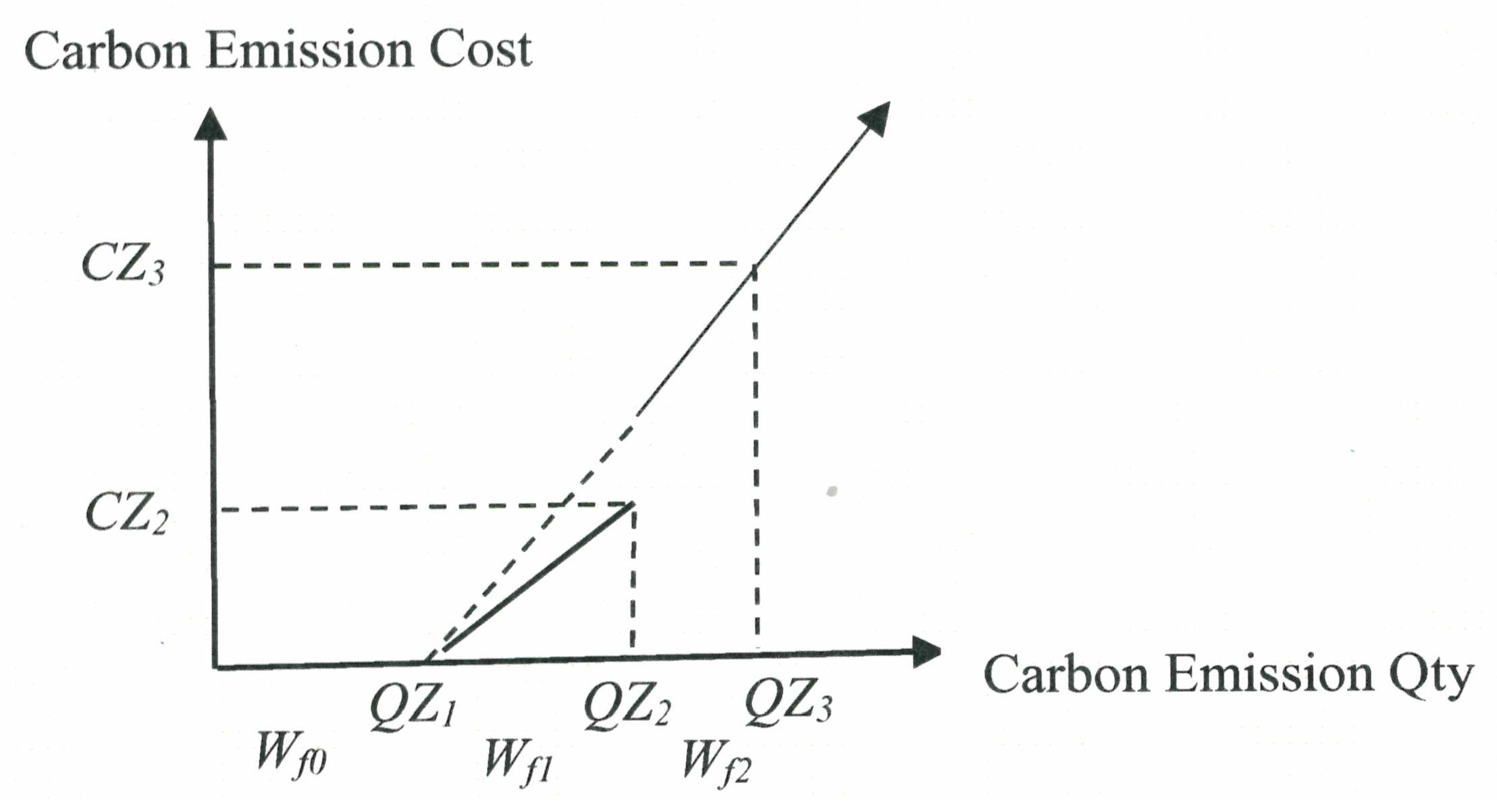
EQf, QZ1, QZ2EQf is the total carbon quantity for factory f, but arrive at QZ1 and QZ2 that its cost is different.
Wf1,Wf2Both are an actual total carbon quantity, Wf1 less than QZ1, Wf2 between QZ1 and QZ2. The f (f = 1 or 4) is only for factory 1 or 4;
CZ2, CZ3That is the total carbon cost for EAF and BF depend on the carbon quantity at QZ2 or QZ3.
RZ, RZ1, RZ2The percent of carbon quantity for producing P1 by EAF or BF; RZ1 for EAF, RZ2 for BF, 4 * RZ1 = RZ2; RZ1 = 40%;
UZ1, UZ2The unit cost of carbon, when arrive at QZ1 and QZ2, respectively;
CIfThe machine costs are fixed for each factory, f index (f = 1,2,3,4);
rpOther indirect costs use each product only as the rp percentage of customer revenue to represent the total amount of other indirect costs, p index (p = 1,2,3);
CGfThe other indirect costs for each factory by using each product only as the rp percentage of customer revenue, f index (f = 1,2,3,4);
Table 3. Designing smart codes for BBB steel group (including conpanies and factories), and assuming the sales forecast for each product (equals target quantities of production).
Company-CodeFactory-CodeSales Forecast (tons)
A-BU/P1B-BU/P2C-BU/P3
QP1 = QP11 + QP14;
qP1 = QP111 + QP112 + QP113
QP2 =
QP21 + QP23
QP3 =
QP32 + QP33
CustomersTransfersIntersegment SalesSalesSales
PCF1QP11QP111 QP21
F2 QP112 QP32
SC1F3 QP113QP23QP33
SC2F4QP14
Table 4. The example data according to Figure 7, designing a measurement report form for BBB corporate group and divide each company into different Business Unit (BU).
DescriptionsPCSC1SC2
F1F2F3F4
P1 (A-BU)P2 (B-BU)P3 (C-BU)P2 (B-BU)P3 (C-BU)P1 (A-BU)
A1. external customersQP11 * UP1QP21 * UP2QP32 * * UP3QP23 * UP2QP33 * UP3QP14 * UP1
A2. intersegment sales QP113 * uP1
A3. transfers (QP111 + QP112) * uP1
A4. byproductsQS1 * US1 QS2 * US2
A.Revenue = A1 + A2 + A3 + A4
B. semi-manufactured goods QP111 * uP1QP112 * uP1QP113 * uP1
C1. Purchasing material QM1 * UM1 QM2 * UM2 + QM3 * UM3
C2. byproduct(QS3 * UM1)QS3 * UM1
C. Material cost
C = C1 − C2 or C = B − C2
( m = 1 3 U M m Q M m ) ( Q S 3 U M 1 ) only for P1 from F1
(QP111 + QP112 + QP113) − (QS3 * UM1) only for P2 and P3
D. Labor costCLs = $ 3696CL1 + δ1(CL2 − CL1) + δ2(CL3 − CL1)CL v = $ 2520
E. Electrical costCE = Ed * X * UE
F. CO2 cost[π1 * UZ1 * (Wf1 − QZ1) + π2 * UZ2 * (Wf2 − QZ1)] only for P1
G. Machine costs f = 1 4 CI f
$42,000$3000$4500$3000$3500$8500
H. Other costs f = 1 4 CG f only for external customers
3% * QP11 * UP15% * QP21 * UP25% * QP32 * UP35% * QP23 * UP25% * QP33 * UP33% * QP14 * UP1
I. Profit = A − C … −H
<Note> 1. Unit price (NTD1000): A1: External customers: UP1 = $14, UP2 = $18 and UP3 = $20.5; A2/A3: Intersegment sales/transfers: uP1 = $13.5; A4: Byproducts: US1 = $0.3 and US2 = $0.03; C1: Purchasing material: UM1 = $9.1, UM2 = $3.2 and UM3 = $2.2. 2. Quantitative constraints of various products: A1: External customers: QP11 ≤ 10,000; QP21 ≤ 17,600; 22,000 ≤ QP32 ≤ 24,000; 14,000 ≤ QP23 ≤ 17,200; QP33 ≤ 19,300; and QP14 ≤ 36,000; A4: Byproducts: QS1 = QM1 − (QP11 + qP1) and QS2 = 0.5 * QP14; B: Semi-manufactured goods: QP111 = QP21 * 1.02; QP112 = QP32 * 1.03; and QP113 = QP23 * 1.02 + QP33 * 1.03; C1: Purchasing material: qP1 = QP111 + QP112 + QP113; QM1 = 1.11 * (QP11 + qP1); QM1 = 100 * X; X ≤ 950; QM2 = 2.9 * QP14; QM3 = 0.9 * QP14; QM2 ≤ 100,000; and QM3 ≤ 50,000.
Table 5. The mathematical programming model and optimal solution (unit NTD1000).
MAX ω = {[(QP11 + QP14) * 14] + [(QP21 + QP23) * 18] + [(QP32 + QP33) * 20.5] + [(QP111 + QP112 + QP113) * 13.5] + [(QS1 * 0.3) + (QS2 * 0.03)]} − {[(QP111 + QP112 + QP113) * 13.5 − QS3 * 9.1] − [(QM1 * 9.1) − (QS3 * 9.1)] + (QM2 * 3.2) + (QM3 * 2.2)} − {3960 + [6600 + r21 * (7837.5 − 6600) + r22 * (9187.5 − 6600)] + [7920 + r31 * (9405 − 7920) + r32 * (11,025 − 7920)] + (1800 + 720) + 3696} − (45 * 2.6 * X) − 64500 − [R11 * 60 * (W11 − 5000)/1000 + R12 * 90 * (W12 − 5000)/1000 − 2100] − [R41 * 60 * (W41 − 5000)/1000 + R42 * 90 * (W42 − 5000)/1000] − [(QP11 + QP14) * 14 * 0.03 + QP2 * 18 * 0.05 + QP3 * 20.5 * 0.05]
Subject to semi-manufactured goods qty:
QP111 = QP21 * 1.02;
QP112 = QP32 * 1.03;
QP113 = QP23 * 1.02 + QP33 * 1.03;
qP1 = QP111 + QP112 + QP113;
QM1 = 1.11 * (QP11 + qP1);
QS1 = QM1 − (QP11 + qP1);
QS2 = 0.5 * QP14;
Subject to sales qty:
QP2 = QP21 + QP23;
QP3 = QP32 + QP33;
QP11 ≤ 10,000;
QP14 ≤ 36,000;
QP21 ≤ 17,600;
14,000 ≤ QP23 ≤ 17,200;
22,000 ≤ QP32 ≤ 24,000;
QP33 ≤ 19,300;
Subject to direct material:
QM1 = 100 * X;
QM2 = 2.9 * QP14;
QM3 = 0.9 * QP14;
QS3 = qP1 − QP2 − QP3;
X ≤ 950;
QM2 ≤ 100,000;
QM3 ≤ 50,000;
Subject to machine hour:
(20 + 60) * X ≤ 176 * 60 * 7;
QP2 * 1.5 ≤ 52,000;
QP3 * 2 ≤ 83,000;
Subject to direct labor for F1:
NL1 = 150;
QP21 * 1.5 ≤ NL1 * 176;
Subject to direct labor for F2:
NL2 = 250;
QP32 * 2 > NL2 * 176;
QP32 * 2 ≤ NL2 * 216;
QP32 * 2 = 44,000 + r21 * (49,500 − 44,000) + r22 * (54,000 − 44,000);
r20 − y21 ≤ 0;
r21 − y21 − y22 ≤ 0;
r22 − y22 ≤ 0;
r20 + r21 + r22 = 1;
y21 + y22 = 1;
Subject to direct labor for F3:
NL3 = 300;
(QP23 * 1.5) + (QP33 * 2) > NL3 * 176;
(QP23 * 1.5) + (QP33 * 2) ≤ NL3 * 216;
(QP23 * 1.5) + (QP33 * 2) = 52800 + r31 * (59400 − 52800) + r32 * (64800 − 52800);
r30 − y31 ≤ 0;
r31 − y31 − y32 ≤ 0;
r32 − y32 ≤ 0;
r30 + r31 + r32 = 1;
y31 + y32 = 1;
Subject to direct labor for F4:
NL4 = 300;
QP14 * 2 > NL4 * 200;
QP14 * 2 ≤ NL4 * 240;
Subject to CO2 Emission for F1:
RZ1 = 0.4;
(QP11 + qP1) * RZ1 = EQ1;
EQ1 = R10 * W10 + R11 * W11 + R12 * W12;
0 < W10 ≤ 5000;
5000 < W11 ≤ 10,000;
10,000 < W12 ≤ 100,000;
R10 + R11 + R12 = 1;
Subject to CO2 Emission for F4:
RZ4 = 1.6;
QP14 * RZ4 = EQ4;
EQ4 = R40 * W40 + R41 * W41 + R42 * W42;
0 < W40 ≤ 5000;
5000 < W41 ≤ 10,000;
10,000 < W42 ≤ 100,000);
R40 + R41 + R42 = 1;
Optimal decision solution/NTD1000/ton:
ω = $536,370.8, QP11 = 1910, QP14 = 34,482, QP21 = 17,600, QP23 = 17,052, QP32 = 24,000, QP33 = 17,500, QP111 = 17,952, QP112 = 24,720, QP113 = 35,418, QS1 = 8800, QS2 = 17,241, QS3 = 1,938, QM1 = 88,800, QM2 = 99,997.8, QM3 = 31,033.8, R21 = 0.7272727, R31 = 0.7818519, R32 = 0.2181481, X = 888, R12 = 1, W12 = 32,000, R42 = 1, W42 = 55,171.2, Y21 = 1, Y22 = 0, Y31 = 0, Y32 = 1,EQ1 = 32,000,EQ4 = 55,171.2;
Table 6. BBB group (by company).
DescriptionsPCSC1SC2
F1F2F3F4
P1P2P3P2P3P4
(A-BU)%(B-BU)%(C-BU)%(B-BU)%(C-BU)%(A-BU)%
A1: External customers26,7402.5316,800100492,000100306,936100358,750100482,74899.9
A2: Intersegment sales478,14344.1
A3: Transfers576,07253.2 0.0 0 0 0 0.0
A4: Byproducts26400.2 5170.1
A. Revenues = A1 + A2 + A3 + A41,083,595100316,800100492,000100306,936100358,750100483,265100
B. Semi-manufactured goods 242,35276.5333,72067.8234,80676.5243,33867.8
C1: Purchasing material808,08074.6 388,26780.3
C2. Byproduct17,636−1.632031.065521.331031.047781.3
Material cost (B − C2) 239,14975.5327,16866.5231,70275.5238,56066.5
Material cost (C = C1 − C2)790,44472.9 388,26780.3
D. Labor cost36960.339601.375001.541201.356381.625200.5
E. Electrical cost103,8969.6 0.0 0.0 0.0 0.0
F. CO2 cost3300 0.0 0.0 0.0 0.045150.9
G. Machine cost42,0003.930000.945000.930001.035001.085001.8
H. Other cost8020.115,8405.024,6005.015,3475.017,9385.014,4823.0
I. Profit = A − C … −H142,42713.154,85117.3128,23226.152,76717.293,1142664,98013.4
<Note> According to Figure 7 and Table 5, Table 6 shows a measurement report form for BBB corporate group in a period and divide each company into different BUs; Unit: NTD1000/ton.
Table 7. BBB group (by BU).
Descriptions(A-BU)%(B-BU)%(C-BU)%Total%
A1: External customers509,48832.5623,736100850,7501001,983,97465.2
A2: Intersegment sales478,14330.5 478,14315.7
A3: Transfers576,07236.8 576,07218.9
A4: Byproducts31570.2 31570.1
A. Revenues = A1 + A2 + A3 + A41,566,860100623,736100850,7501003,041,346100
For: Reportable segments52% 20% 28% 100%
B. Semi-manufactured goods 477,15876.5577,05867.8
C1: Purchasing material1,196,34776.4
C2. Byproduct−17,636−1.163061.011,3301.3
Material cost (B − C2) 470,85175.5565,72866.51,036,57934.1
Material cost (C = C1 − C2)1,178,71275.2 1,178,71238.8
D. Labor cost62160.480801.313,1381.527,4340.9
E. Electrical cost103,8966.6 0.0 0.0103,8963.4
F. CO2 cost48450.3 0.0 0.048450.2
G. Machine cost50,5003.260001.080000.964,5002.1
H. Other cost15,2851.031,1875.042,5385.089,0102.9
I. Profit = A − C … −H207,40713.2107,61817.3221,34626.0536,37017.6
<Note> According to Figure 8 and Table 5, Table 7 consolidates the same BU measurement report of different companies in the BBB group in a period; Unit: NTD 1000/ton.
Table 8. Unit and cost structure analysis of P1.
DescriptionsPCSC2
F1F4
P1External%Internal%P1External%
(A-BU)UnitUnit(A-BU)Unit
External sales Q’ty1910 34,482
Internal sales Q’ty78,090
A1: External customers26,74014.00100 482,74814.00100
A2: Intersegment sales478,143 13.5100
A3: Transfers576,072
A4: Byproducts2640 517
A. Revenues = A1 + A2 + A3 + A41,083,595 483,265
B. Semi-manufactured goods
C1: Purchasing material808,080 388,267
C2. Byproduct−17,636
Material cost (B − C2)
Material cost (C = C1 − C2)790,4449.8870.589.8873.19388,26711.2680.43
D. Labor cost36960.050.330.050.3425200.070.52
E. Electrical cost103,8961.309.281.309.62
F. CO2 cost3300.000.030.000.0345150.130.94
G. Machine cost42,0000.533.750.533.8985000.251.76
H. Other cost8020.423.00.00 14,4820.423.00
I. Profit = A − C … −H142,4271.8313.041.7512.9364,9801.8713.35
<Note> Unit: NTD 1000/ton.
Table 9. Sensitivity analysis on the carbon emission reduction goal.
Unit: NTD 1000/ton
ULCEQDecrease ULCEQProfitDecrease Profit
88,000-536,370.8-
87,500-536,370.8-
87,171.2-536,370.8-
87,000−171.2536,130.2−240.6
86,500−671.2535,444.4−926.4
86,000−1171.2534,760.8−1610.0
85,500−1671.2534,075.0−2295.8
85,000−2171.2533,391.4−2979.4
84500−2671.2532,705.7−3665.1
84,000−3171.2532,022.1−4348.7
83500−3671.2531,336.3−5034.5
83,000−4171.2530,652.7−5718.1
82,500−4671.2529,966.9−6403.9
82,000−5171.2529,283.3−7087.5
81500−5671.2528,597.5−7773.3
81,000−6171.2527,913.9−8456.9
80500−6671.2527,228.2−9142.6
80,000−7171.2526,544.6−9826.2

