Abstract
Key performance indicators (KPI) are widely used tools to evaluate the economic (in)efficiency of services, including the ones devoted to urban solid waste management. Regulatory exercises are, then, mostly based on the outputs from KPIs, raising some questions about their validity. In theory, other more appropriate tools could be used to estimate those efficiency levels. This study evaluates the economic inefficiency level of urban solid waste management services in Portugal (2010–2017) through the adoption of partial frontier benchmarking models (order-m) coupled with weight restrictions. That way, the constructed model can evaluate the performance of those services under some regulatory and sustainability requirements. Then, estimated efficiency levels and some common KPIs are compared in order to understand if the latter are sufficient to explain the economic efficiency. The novelty of this research lies in two main aspects: (a) the utilization of a robust order-α model coupled with weight restrictions linked to regulatory and sustainability impositions to estimate efficiency, and (b) the comparison of economic efficiency and some commonly used KPIs, including waste fractions and recycling rate. Results point towards efficiency distributions that follow Weibull functions, with the average close to 50%; thus, nearly half of the resources have been well spent in municipal solid waste management services since 2010 onwards. Nonetheless, in an efficient system, that average would be close to 100%. Additionally, the considered management related KPIs do not exhibit any relationship with economic efficiency, which means that their interpretation and usefulness for regulatory issues are both limited and should be used carefully. In other words, those KPIs are not good performance drivers and carry no capacity to explain economic (in)efficiency in urban solid waste management services.
1. Introduction
To the extent that society consumes more and more material and requires more resources, it also unequivocally generates more waste [1,2]. With the dramatic increase in waste and the emerging need for care, standardization of waste classification criteria has become necessary [3]. There are multiple definitions of Urban or Municipal Solid Waste (MSW) [4]. Eurostat, for instance, adds that MSW includes not only waste collected “by or on behalf of municipal authorities” but also the waste collected “by the private sector (business or private non-profit institutions) not on behalf of municipalities” [5]. The definition of MSW can be ambiguous and may vary from country to country [6], mirroring various waste management practices [7,8,9].
Present times are characterized by a consumerist society [10]. The industrialization and modernization of the economy resulted in excessive consumption habits and in a consequent increase in waste production [11], in both quality and quantity terms, as waste increased not only in number but also in complexity, with more toxic materials and more hard materials to biodegrade [4,12].
Over the past decades, European policies devoted to this sector have been through rapid changes. In Portugal, for instance, these changes can be blamed for the serious environmental dysfunctions, the scarcity of appropriate waste disposal sites, the rising costs of collection and treatment systems, and even society’s increased awareness of environmental issues [10]. For the sake of sustainability, understanding the economic efficiency of municipalities in terms of MSW management appears to be a cornerstone for the regulator (ERSAR, standing for the Entidade Reguladora dos Serviços de Água e Resíduos, the Portuguese words for Water and Waste Services Regulatory Authority).
Measuring the performance of services devoted to waste management (collection and treatment) very often requires the utilization of robust mathematical models that can compare comparable services to each other. Perhaps due to lack of knowledge or appropriate tools, public entities, including regulators, usually lay their analyses on the utilization of key performance indicators (KPI). Usually, KPIs result from simple indicators, such as quantity of collected MSW per currency unit spent or the weight of recycled waste on the total collected MSW. A problem related to the utilization of KPIs is that they frequently raise more questions than provide answers about the performance of those services (a service can be the best performer in one KPI and the worst in another). Solving such a problem may require multicriteria decision analysis tools that result in questionable outputs, provided the subjective nature of appreciations of each stakeholder.
For sustainability issues, there is thus a major question: “Whenever measuring (economic) efficiency, should we be satisfied with easily estimated KPIs?”. Associated with this, one should wonder whether using robust mathematical models, namely the benchmarking related ones, will bring different and better outputs for the regulatory exercise. To answer the question “Do KPIs and economic efficiency provide the same outputs?” is, then, one of the goals of this study.
Answering the question above requires the utilization of a benchmarking model for economic efficiency estimation to compare its outputs with the KPIs and test whether they are statistically similar. This study centers itself on benchmarking models that construct efficiency frontiers, where efficient MSW services are positioned therein. Frontier-based benchmarking models are typically classified into parametric and non-parametric, depending upon the need for specifying a functional form for the frontier or not, respectively. Stochastic frontier analysis is an example of a parametric model. Data Envelopment Analysis (DEA), in opposition, is a non-parametric model. From DEA some other models have been proposed in the literature, namely the Free Disposal Hull (FDH). In the case of non-parametric models, the frontier results from optimization models that are based on the dataset only, being thus more flexible and making no strong assumptions about the frontier. Therefore, instead of imposing a functional form for the frontier, this study focuses on non-parametric models.
Both DEA and FDH estimate full frontiers, which envelop the entire sample and, because of that, are sensitive to outliers and extremes. In opposition and still being non-parametric, the so-called partial frontier models are noteworthy because they do not envelop the entire sample of services. They are, thus, less sensitive to the presence of outliers that shift the frontier, wrongly underestimating the efficiency of the remaining observations. There are two models that estimate partial frontiers: order-m and order-α. They require the definition of a single parameter: m or α, respectively. Parameter m states the number of potential benchmarks associated with each MSW service. Parameter α indicates the probability of observing points outperforming the frontier. Hence, its interpretation is easier in practice than that of the parameter m (from order-m).
This study focuses on order-α to estimate the economic efficiency of Portuguese MSW services. It is often desirable to include restrictions in benchmarking models to impose regulatory and sustainability requirements, such as the reduction of MSW disposable in the landfill and simultaneous increase of recycling and valorization of waste. In other words, between two MSW services collecting the same quantity of MSW and spending the exact same money for that, the one recycling and/or valorizing more waste compared to landfilled waste is more efficient. The introduction of these regulatory and sustainability requirements can be made through weight restrictions in order-α, demanding for a complex mathematical model based on Monte-Carlo algorithms.
This paper’s goals are threefold:
- Goal 1
- To estimate MSW management services’ economic efficiency, through the robust order-α model, and using Portugal as the case study;
- Goal 2
- To insert weight restrictions into the order-α model to couple the economic efficiency analysis with some regulatory and sustainability requirements;
- Goal 3
- To compare the economic efficiency of MSW management and some of its common KPIs.
Accomplishing these goals constitutes the novelty of this manuscript. It is expected that our results will help regulators and policy-makers to design better strategies and policies to enhance the waste sector and its sustainability.
2. The Urban Solid Waste Sector in Portugal
Several authors have mentioned that the search for a strategy to encourage lower waste production only began in 1985 in Portugal [13]. According to Marques and Simões [14], it was from the 1990s onwards that problems such as improper waste management led the government authorities to pay more attention to this problem.
Nevertheless, policies at the time were more focused on collection than on treatment and destination. Some laws were imposed and part of them were transposed from the internal legal order of the EU Directives [6]. Strategies to encourage lower waste generation meant that the waste producer should properly collect, store, transport, dispose of, and use waste without endangering human health or causing harm to the environment. The first Strategic Plan for MSW (PERSU I) was approved in 1996, and has successively been updated until the present [6,15,16,17]. PERSU 2020 is the current Strategic Plan for MSW, having been launched in 2014. It is expected to end in 2020 to address the need to align the achievement of goals strategy with the Portuguese national policy of MSW as well as to adapt to changes in waste management systems and in community targets.
Based on Tchobanoglous et al. [18] and McDougall et al. [19], waste management systems must ensure both environmental and economic sustainability, minimizing environmental impacts, while maintaining costs that are acceptable to the community, citizens, businesses, and governments. Waste management systems in Portugal are segmented into two categories according to the activities they perform, being classified as ‘low’ or ‘retail’ and ‘high’ or ‘wholesale’. The ‘retail’ segment comprises the process of collecting waste that municipalities are responsible for, from disposal sites to transfer stations or to a treatment plant. The ‘wholesale’ system involves operations that start at transfer stations until final landfilling or other treatment destination and is usually the responsibility of the regional operators. They often involve more than one municipality due to the high costs involved in the transfer and final disposal of waste. Currently in Portugal, the ‘retail’ service has 255 operators, while the ‘wholesale’ service has 23, as it usually involves more than one municipality due to the high costs involved in the transfer and final disposal of waste.
In addition, both ‘retail’ and ‘wholesale’ operators have different management models. The management models can be concessions, delegated management, or direct provision [20]. More specifically, for ‘retail’ services, the management model is either delegated to municipal/intermunicipal companies, or the management is direct and done by municipalities or done by association of municipalities. The predominant management model is the direct management carried out by each municipality, (228 of the 255 operators). The wholesale service often involves more than one municipality due to the high costs, and for this reason, the 23 operators that manage these activities can be delegated by municipal/inter-municipal companies, or direct management by associations of municipalities.
MSW services are public and essential for the well-being of citizens, public health and the collective safety of the population and their access must be governed by the principles of universality, continuity, and quality of service, and price efficiency and equity [21]. Besides, in Portugal, MSW services are provided under a legal monopoly. As a rule, in each geographical area there is only one service provider. Nevertheless, the competition in the industry is naturally conditioned by the fact that the user can neither choose the management model nor the price/quality. To prevent entities from inflating prices, regulation is fundamental to defend the interests of end-users. For these reasons, the sector must be regulated. In Portugal, the regulatory authority for wastewater and municipal waste, ERSAR, performs regulatory functions over all mainland Portugal operators and works a state intervention tool.
Regarding urban waste management, the following definitions are used in the paper:
- Collection method: The collection of waste, including the preliminary sorting and storage of waste for the purpose of transport to a waste treatment facility. By collection method, waste can be categorized into refuse and selective waste.
- ○
- Refuse (or unsorted) waste: This covers the collection and transportation of all kinds of waste simultaneously, without separation. Waste is placed in the same container.
- ○
- Selective waste: This refers to the (separated) collection and transportation of waste of specific types, placed in specific containers. It includes glass, paper and cardboard, metal, plastic, packaging, and batteries. It also considers the biodegradable waste (cooking oils) conducted for organic recycling, and the waste collected door-to-door, recycling centers, and special circuits, which are increasingly common. This is the case, for example, mattresses, refrigerators, couches, electronic and electric equipment, textiles, among others.
- Destination: Once collected, waste can be landfilled, valorized, or recycled.
- ○
- Recycled waste: Waste materials recovered, i.e., reprocessed into products, materials, or substances either for the original purpose or for other purposes. This category does not include the valorized waste that results into heat, compost, or biogas.
- ○
- Valorized waste: This can be either energetic or organic.
- ▪
- Energetic valorization: Also named energy recycling, it is the use of combustible waste to produce energy from direct incineration with heat recovery.
- ▪
- Organic valorization: This refers to the use of the organic fraction contained in waste to produce compost (aerobically) or biogas and compost (anaerobically). The final product (the compost, or fertilizer) is stable and harmless. It is in a state of total or partial humidification that allows its introduction into the soil in a compatible way.
- ○
- Landfilled waste: Waste disposal in landfills includes the MSW, which is nether recycled nor valorized.
3. Literature Review
Several authors have used KPIs to analyze the performance of MSW services. Thirteen relevant studies are presented below. These studies have been selected because they met the following three criteria: (a) contemporaneousness, i.e., they were published after 2005, (b) significance, i.e., they were published in a peer review International Scientific Indexing (ISI) journal, and (c) clarity, i.e., they explicitly identified the KPIs to monitor MSW services management or make a comprehensive review of these KPIs, identifying them as well.
Suttibak and Nitivattananon [22], for instance, used KPIs associated with efficiency, effectiveness, and service ratio for the assessment of recycling performance. The purpose was to investigate the factors influencing the performance of MSW management related to solid waste recycling, covering a total of 120 solid waste recycling programs located in different urban areas of Thailand.
Guimarães et al. [23] suggested the use of tools such as balanced scorecard in the measurement of the performance of MSW companies and added that despite the inevitability of price increases, it is necessary to reinforce the improvement in the efficiency of operations, which will force concessionaires to improve their procedures, their communication policy, and manage the urban waste collection service as a business that, above all, serves its customers.
Considering that there is a growing appeal for an active involvement of municipalities with regard to solid waste, Mendes et al. [24] mentioned the importance of specificities in the performance assessment and decision-making context of municipalities regarding sustainability strategies and policies. The maturity of the municipality in the management of their solid waste as well as the seasonality level, due to the existing specificities, are important factors in measuring the level of performance.
Zaman [25] listed several MSW management KPIs based on past studies. The author conducted a survey with waste professionals from different sectors and countries and categorized in seven different domains the zero waste performance indicators, identifying 56 indicators as the most important.
Parekh et al. [26] evaluated the performance of the MSW management system using 44 KPIs, identified by brainstorming sessions, structured interviews, and group discussions with experts. To assign weights per KPI they used the Analytical Hierarchy Process. Those KPIs were classified into eight main areas of MSW management for performance measurement: (1) coverage; (2) transportation; (3) disposal; (4) consumers’ complaint; (5) unitary cost; (6) outcomes; (7) segregation, recovery and recycling; and (8) environmental factors.
Teixeira et al. [27] used KPIs to evaluate the independent operational and economic efficiency and performance of municipal MSW collection practices. Those indicators were then used in life cycle inventories and life cycle impact assessment. The life cycle assessment environmental profiles provided the environmental assessment. They applied this tool to the Portuguese city of Oporto, as a case study.
Sanjeevi and Shahabudeen [28] conducted a literature review on MSW management systems, especially on KPIs, and suggested practical management methods based on those identified studies. To capture the essential parameters that need to be monitored in a simplified manner, the authors identified the main KPIs that have been used over the years.
Yang et al. [29] measured and compared the aggregate urban efficiency of 22 administrative regions of Taiwan using DEA. Instead of using a single-ratio indicator, their study applied an integrated framework to evaluate the aggregate urban input–output (or economic) efficiency.
Martinho et al. [30] used recycling and logistic performance KPIs collected during a field campaign by a team that characterized the waste, and also a survey of citizens living in the neighborhoods allowed them to calculate the participation rate indicator. The methodology was based on the characterization campaign from the National Strategy Plan of Municipal Solid Waste II, of Portugal, and the results show that the mixed collection system yields higher material separation rates, higher recycling rates, and lower contamination rates.
Rodrigues et al. [31] adapted a methodology for Multi-Critical Decision Aid—Constructivist, emphasizing the weights attributed by experts in defining KPIs to integrate them into the model and obtain a global classification that can be used as benchmarking in measuring and comparing the proposed strategic objectives for MSW management. Based on the representativeness of the performance indicator spectrum made by the authors, they chose both quantitative and qualitative KPIs covering fundamental sustainability issues and enabling the delimitation of an application domain for overall performance of waste management.
Also based on KPIs, and more recently, Cetrulo et al. [32] conducted an empirical statistical analysis over panel data to assess the effectiveness of the municipal Brazilian solid waste policy and whether the indicators improved or not (considering the ex-post policy effectiveness evaluation). The effect indicators selected included (a) waste generation per capita as the municipal waste generation indicator; (b) collection coverage and collection frequency as municipal waste collection indicators; (c) recovery rate of recyclable waste as the recycling rate indicator; and (d) rate of proper disposal as the MSW final disposal method indicator.
In the same year, Bertanza et al. [33] suggested a set of indicators that overcome the limitations of some aspects that influence the operational efficiency on the collection service, taking into account both the characteristics of collected waste and the operational–economic performance. Considering the approach used, they defined three groups of indicators, highlighting the impact of the main factors that influence the operational performance of the collection strategies and which are related to personnel, vehicles, and containers: (1) performance indicators; (2) economic indicators (3), descriptive indicators.
Through the use of bibliometric indicators, bibliographic survey, and content analysis of articles published until July 2017, by different authors and institutions from different countries, Deus et al. [34] identified which KPIs are involved in MSW management. According to the authors, Portugal, for example, had seven publications and occupied the sixth position of the rank, with ten local citations score and sixty global citations score.
Based on the previous studies, we conducted a frequency analysis of KPIs used therein. The initial counting of KPIs was 195. The KPIs were grouped by categories similarly to Zaman’s approach [25]. Some of the KPIs were specially dedicated to particular cases of each MSW management system and may vary in line with the data available in each case. Hence, to facilitate this analysis we conducted a generalization of indicators of the same scope and reduced KPIs from 195 to 135. Figure 1 shows the share of indicators per category. Seven main categories were identified: management (46% of the KPIs used), economic (17%), organization (13%), governance and customers/consumers (11%), geo-administrative (6%), environment (5%), and socio-cultural (2%). Management related KPIs were the most employed. Figure 2 presents the 32 most popular KPIs among the studies surveyed. Most of those indicators regarded management and included (but were not limited to): waste fraction, waste per capita, separation rate, and collection frequency.
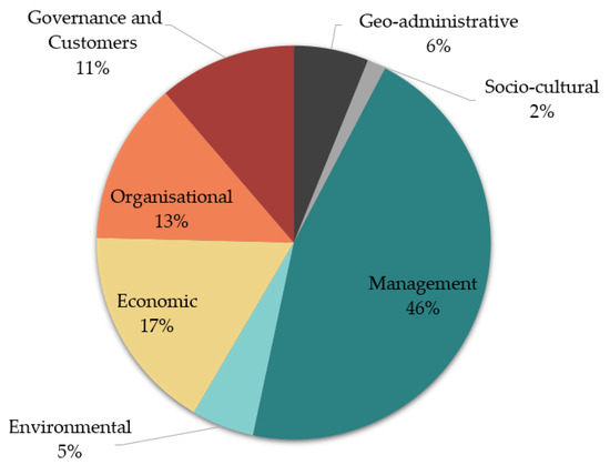
Figure 1.
Share of indicators by categories.
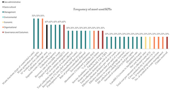
Figure 2.
Frequency of the most-used key performance indicators (KPIs).
It is interesting to note that none of those studies compared the KPIs with economic efficiency estimated through robust benchmarking methods coupled with regulatory and sustainability requirements to effectively understand whether such KPIs are good proxies for efficiency. This is a major critique of the surveyed studies, because the KPIs are only partial productivity measures. Without a proper aggregation metric, as conducted by benchmarking models or multicriteria decision analysis, the analysis of KPIs may result in misleading conclusions about the MSW services’ performance.
Our further analysis will be based on some management related KPIs. The KPIs used therein are easily computable based on raw data that are used to estimate efficiency as well. That way, comparisons are not likely to be biased due to factors other than the distinct models used to construct the economic efficiency scores and the KPIs (whose data sources are the same). Four of the most common KPIs—or a transformation of them—will be considered, among others: waste fractions [24,25,26,30,33], separate waste collection rate [25,26,30,33], recycling rate [24,26,28], and total cost per amount of collected waste [24,33].
4. Methodology
4.1. Inputs and Outputs
Economic (in)efficiency estimation through benchmarking models demands the adoption of inputs (or resources), x, and outputs, y, i.e., the result of the productive process. We considered two models for efficiency assessment. Using two models was intended to improve the robustness of our analysis and conclusions. These models shared the same input, x, which was the municipal spending on MSW management. Nonetheless, they differed on the outputs:
- Model A.
- y1, quantity of selective waste collected; y2, quantity of refuse waste collected;
- Model B.
- y3, quantity of landfilled waste; y4, quantity of recycled waste; y5, quantity of waste with energetic valorization; y6, quantity of waste with organic valorization.
Hereby, quantities of collected waste will be expressed in tons, while spending on MSW management will be expressed in thousand €. Using this input, x, and these outputs, yr (r = 1, …, 6), we employed a benchmarking model (the order-α with weight restrictions) to assess the economic efficiency of MSW collection and treatment. By comparing two efficiency measures (conditional and unconditional) it would be possible to understand the behavior of efficiency when one (or more) of those KPIs changed. Figure 3 presents the path conducted to reach such a goal.
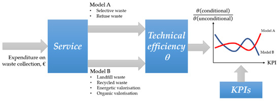
Figure 3.
Flowchart.
4.2. Key Performance Indicators
This study aimed at establishing the link between MSW services’ economic efficiency on MSW management and KPIs. Based on the previous literature review, available data, and the easiness of computation, ten KPIs were selected. KPIs 1 to 6 were intended to measure the operational efficiency (ratio between an output and the spent resources to reach that). KPIs 6 to 10 tried to measure the effectiveness of recycling and valorization policies. Table 1 details the computation of those ten KPIs. They were defined as follows:

Table 1.
Computation of KPIs.
- KPI 1.
- Tons of collected MSW per thousand € spent by the service;
- KPI 2.
- Tons of selective waste collected per thousand € spent by the service;
- KPI 3.
- Tons of refuse waste collected per thousand € spent by the service;
- KPI 4.
- Tons of landfill waste per thousand € spent by the service;
- KPI 5.
- Tons of recycled waste per thousand € spent by the service;
- KPI 6.
- Tons of valorized waste (either organic or energetic) per thousand € spent;
- KPI 7.
- Weight of selective waste on total collected MSW;
- KPI 8.
- Weight of refuse waste on total collected MSW;
- KPI 9.
- Weight of recycled waste on total collected MSW;
- KPI 10.
- Weight of valorized waste (either organic or energetic) on total collected MSW.
4.3. The Order-α Model for Economic Efficiency Assessement
There are several alternatives to cross economic efficiency and a set of variables that can explain part of the former’s variance. This study used KPIs as potential explanatory variables for economic efficiency. Perhaps the most common alternative to cross those dimensions is the (either multiple or simple) regression, using efficiency as the dependent variable, regardless of the model used to estimate such an efficiency. However, it has been reported in the literature that regression, either using bootstrap or not, cannot properly explain efficiency distributions or the reason why best practices belong to the frontier, i.e., are efficient. This is because regression relies on the so-called separability condition, which is to say that the production process is not influenced by the selected explanatory variables [35,36,37,38,39,40,41]. Unless there is a strong reason supporting the separability condition, regression analyses should be avoided to explain economic efficiency. Instead, the order-α model [35] attempted to solve this problem, considering the potential explanatory dimensions (such as KPIs) as part of the productive process, and then turning it useful for the empirical analysis carried out by this study.
This subsection, thus, details the order-α model for economic efficiency assessment in the presence of weight restrictions and “external” conditions. The authors developed and ran Matlab® codes to estimate the economic efficiency of Portuguese MSW management services. These codes can be made available upon request. Matlab® is a high-performance software (available: https://www.mathworks.com/products/matlab.html) widely used by the research community and useful to program optimization-based routines, required in this study.
4.3.1. The Unconditional Order-α Model
Order-α is a benchmarking model that imposes a probability 1 − α of observing points outperforming the frontier (these are deemed outliers or extreme values) [35]. Instead of constructing a full frontier, as other models do, including the well-known Data Envelopment Analysis (DEA) and Free Disposal Hull (FDH) [36], the order-α constructs a partial frontier because not all observations are “enveloped” by it. For this reason, such a model is much more robust to the outliers and extreme observations than full frontier models. In addition to this, the mathematical model is not so complex as it does not require linear programming solving tools, but rather some simple matrix computations. Also, the inclusion of the operational environment to adjust or correct the efficiency is quite easy to perform. Nonetheless, the original model does not allow for the inclusion of weight restrictions that are important because of regulatory and sustainability issues. Overall, the main use of order-α, as any benchmarking model, is to estimate efficiency scores for observations. These scores are, roughly speaking, the reciprocal of the distance of those observations to the constructed frontier.
Recently, Ferreira and Marques [37] have shown how to modify the order-α model so as to include weight restrictions and make or test assumptions over operations’ scale others than variable returns to scale. According to those authors, FDH is behind order-α, meaning that any operation allowed over the former (including weight restrictions) can resonate in the latter. Note that FDH can construct a frontier and estimate efficiency scores through a linear program given by Equation (1):
where are multipliers (weights) associated with the service k, featured by the input(s) xk and the output(s) yk, and whose economic efficiency is being assessed. This model assumes the variable returns to scale, which is a flexible assumption that does not require that observations (MSW services, in the present case) operate at similar scales to be compared.
The model of Ferreira and Marques [37] is, however, very complex and difficult to implement and does not compare with the easiness of the original order-α model in which only the parameter α must be defined a priori. To mitigate such complexity, we made use of the correspondence between the order-α and another partial frontier-based model—the order-m [38]—that requires the definition of a parameter m, establishing the number of potential peers for the MSW service under analysis. We know from the literature that should , then both models are equivalent [39]. Although computationally demanding, the inclusion of weight restrictions in order-m is much easier than in the model of Ferreira and Marques [37] (see, for instance, the work of Daraio and Simar [40]). Making the appropriate choice of the parameter α (vide infra), we could establish and run the following model to assess the efficiency of municipality k (out of n) featured by the pair (xk, yk):
- Step 1.
- Define b ← 1;
- Step 2.
- Identify the observations verifying y ≥ yk;
- Step 3.
- From the subsample of observations retained from Step 2, randomly and with reposition select m observations;
- Step 4.
- Use Equation (1) to estimate the efficiency of municipality k against the frontier constructed using the m observations of Step 3 (Equation (1) can be updated to account for weight restrictions);
- Step 5.
- If b < B, update b ← b + 1; otherwise, stop.
At the end of this procedure, we obtained B potentially different efficiency scores. B should be a large quantity, e.g., 5000 iterations. The final efficiency score resulted from the (truncated) average of those B potential efficiency estimates.
Since previous procedure disregards the operational environment, the efficiency score, , is called unconditional, being represented by . The next subsection explains how to include such environmental data into the analysis and, therefore, to obtain the so-called conditional efficiency score, .
4.3.2. The Conditional Order-α Model
One of the greatest advantages of the order-α model is its flexibility in accounting for the operational environment surrounding the MSW service (or any other entity under consideration). Once this aspect has been accounted for, the resulting efficiency score is called conditional, , as it carries a factor correcting for the environmental bias.
Let h be a bandwidth, f an operational environment-related variable, and K a kernel function, such that K((f − fk)/h) = 1 if f ranges from fk − h to fk + h, and K((f − fk)/h) = 0 otherwise. K acts like a bounded probability density function, centered on fk, to be used in Step 3 of the Monte-Carlo routine elicited in Section 4.3.1 during the random drawing process. This implies that the observed values of the m drawn observations in the variable f must belong to the interval [fk − h; fk + h] and, by consequence, those observations and the MSW service k operate in similar environments. Note that the unconditional efficiency estimation results from because previous interval gets unbounded.
4.3.3. On Including Weight Restrictions
The order-α model, born from the well-known nonparametric method FDH, inherently assigns weights to the inputs and outputs in order to optimize the economic efficiency score of the MSW service under analysis. Therefore, the larger the weight of a specific variable (input/output), the higher its impact on such a score. This means that services with large amounts of landfilled and/or refuse waste (compared to selective, recycled, and/or valorized waste quantities) can be highly efficient, if the weights assigned to y2 and y3 optimize (maximize) the efficiency score. Because of sustainability issues, it is compulsory to ensure that (WR stands for weight restrictions):
- WR 1
- The weight assigned to y1, quantity of selective waste collected, should be larger than the one assigned to y2, quantity of refuse waste collected: u1 > u2;
- WR 2
- The weights assigned to y4, quantity of recycled waste, y5, quantity of waste with energetic valorization, and y6, quantity of waste with organic valorization, should all be larger than the one assigned to y3, quantity of landfilled waste: u4 > u3; u5 > u3; and u6 > u3.
Weight restrictions are additional constraints to the FDH mathematical model (1) inserted into the order-α model itself. Such additional constraints limit the flexibility of FDH, hence contributing to a better discrimination of efficiency results.
4.3.4. How to Define the Appropriate Value for α (and m)?
Order-α is useful to mitigate the effect of outliers and extreme observations on efficiency estimation because of the construction of a partial frontier that solely depends on the value of parameter α. The difference 1 − α is the probability of observing MSW services (observations) outperforming the frontier and, then, being potential outliers. Hence, to estimate efficiency, we selected a value of α such that 1 − α is close to 5%. Note here that m denotes the size of the subsample used to estimate the B distinct efficiency scores in the Monte-Carlo algorithm of Section 4.3.1 and, as such, should be at least three times the number of variables used (inputs and outputs). No more than five variables were considered, meaning that , which corresponds to α = 0.96 and 1 − α of 4%. As α tends to 1, then the frontier becomes a full frontier. This is, of course, equivalent to imposing m tending towards infinity.
However, that is not the only advantage of order-α, as it can adjust economic efficiency by the operational conditions in which MSW services operate. Services become comparable even though some may operate in more or less advantageous conditions. Besides this, to study the impact of such conditions on economic efficiency distribution or the relationship between them, Badin et al. [41] advocated the need for looking at the medium frontier, i.e., the partial frontier obtained for α = 0.50 or, equivalently, m = 1.
4.4. On Relating Economic Efficiency and KPIs
To relate economic efficiency with a given KPIp, p = 1, …, 13, we take advantage of the ratio between the conditional and unconditional efficiency estimates. In this case, the KPI took the place of an operational environment variable in order to assess the conditional version of the order-α efficiency score. Consider the following ratio:
If α approaches to 1, then relates to two efficiency scores assessed regarding two full frontiers. Let H0 be the null hypothesis stating that and H1 the alternative hypothesis such that . Should we not reject the null hypothesis in the light of statistical evidence, then we may expect that the KPIp plays no meaningful role on the frontier, i.e., municipalities can be economically efficient regardless of the value of the KPIp. Otherwise, there is a shift on the frontier and the KPIp itself is related to the efficiency profile of MSW services.
Nonetheless, evaluating the impact of the KPIp on the frontier represents just half of the work, as it may also impact on economic efficiency distributions. As claimed before, to evaluate such an effect, we considered the median frontier obtained when α = 0.50. In this case, the new two hypotheses to be evaluated were H0: , meaning that no influence of KPIp on the economic efficiency distribution was expected, against H1: . To understand the relationship of the pth KPI and the economic efficiency distribution, we should look at the trend of the function such that , being and a residual term. The function can be determined via Nadaraya-Watson non-parametric regression. The first derivative of highlights its trend when the pth KPI changes, providing useful information about the relationship between efficiency and the KPI. Should that derivative be equal to zero, then the KPI exhibits no relationship with economic efficiency. Otherwise, the KPI can be understood as unfavorable or favorable to the production process, acting as an undesirable output or freely available substitutive input, respectively. It depends on the sign of the derivative [41].
5. Case Study
5.1. Sample
Our sample was originally composed of the 308 Portuguese MSW services (municipalities, associations of municipalities, or multi-municipal entities), observed for eight years (2010–2017), which resulted in 2464 observations. That is, our initial dataset was composed of the entire universe of Portuguese MSW services, observed over the years. Due to considerable missing data for 26 entities, the latter were removed from the database, reducing its size to 2438 observations, evenly distributed by the time lag. Data were retrieved from the Statistics Portugal (data source: https://ine.pt/, the website of the Statistics Portugal, i.e., the entity that officially collects and treats statistics in Portugal). This official database contains a considerable number of indicators relevant to study the MSW management in Portugal.
5.2. Descriptive Statistics
Table 2 and Table 3 provide the descriptive statistics associated with data of Models A and B, correspondingly. Descriptive statistics as the ones presented therein were obtained through the software SPSS ®, version 25.0 (available: https://www.ibm.com/analytics/spss-statistics-software), which is widely used for statistical analysis among the research community as well as policy-makers and companies. In general, the quantity of selective waste collected is much smaller than the quantity of refuse waste. The former represents, on average, less than one-fifth of the total waste collected. Similarly, landfilled waste still constitutes the biggest fraction of waste, despite its weight in total waste decreasing over the years. It is also interesting to verify that the standard deviation in all variables was recurrently larger than the average. This means that Portugal and its municipalities are very heterogeneous, leading to a broad spectrum of economic efficiency levels and distinct groups of homogenous observations.
Table 2.
Descriptive statistics associated with variables used in Model A. Municipal spending is expressed in thousand €. Quantities of collected waste are expressed in tons.
Table 3.
Descriptive statistics associated with variables used in Model B. Municipal spending is expressed in thousand €. Quantities of collected waste are expressed in tons.
To complement such an analysis, Figure 4 portrays three bar plots exhibiting the annual average of collected waste as well as of four remarkable KPIs. According to these graphs, on average, there was little variation in all the variables, over time. However, in 2013, all variables reached their minimum levels. These values can be related to the conditions of Portugal that, in the very same year, was at the peak of an economical and financial crisis, reflected in the saving of household resources and, consequently, an increase in commitment to waste reduction and recycling. The increase in consumerism by families is related to more produced waste. Nevertheless, we also see that the ability/weight to recycle (selective) was improved over the years.
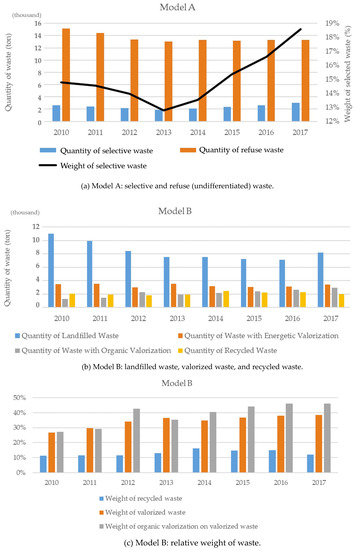
Figure 4.
Bar plots exhibiting some descriptive statistics associated with the variables used in Models A and B.
Table 4 and Table 5 provide the Pearson’s correlation coefficients for the variables used in Models A and B, respectively. In general, the quantity of collected waste was positive and significantly correlated to the expenses. This is, of course, an expected result, as the larger the municipality, the larger the quantity of waste produced, and the more resources must be spent to collect them. The correlation is not perfect (in the sense that it is not exactly equal to 1), as typically municipalities do not operate at their optimal or most productive scale sizes (some may be below while others may be above that optimal scale size). This implies, among other things, that using KPIs, particularly KPI1, will provide no information about scale of operations and any deviation to the “benchmarks” is attributed to inefficiency and/or inappropriateness of practices, and not because of scale.
Table 4.
Pearson’s correlation coefficients for the variables used in Model A.
Table 5.
Pearson’s correlation coefficients for the variables used in Model B.
Organic valorized waste seemed to have weak associations with other variables related to collected waste, inclusively with collection-based expenditures. Landfilled waste also seemed to have a weak, almost meaningless link with such consumed inputs, which instead were highly correlated with recycled waste as well as with waste with energetic valorization. The latter and landfilled waste shared no (linear) relationship.
MSW services seemed to exhibit a common profile in terms of expenses and quantity of collected waste during the considered eight years. To determine whether this hypothesis should be rejected or not, we applied the one-way ANOVA technique, followed by a post-hoc test with the Bonferroni correction. At the 5% significance level, statistical evidence from the ANOVA technique suggests:
- Model A.
- There were no differences either in terms of expenditures or quantity of selected/refuse waste (F < 1.04, p > 0.396).
- Model B.
- MSW services have considerably changed the quantity of landfilled waste (F = 3.39, p = 0.001) as well as the waste with organic valorization (F = 2.70, p = 0.009). Neither the quantity of recycled waste nor of waste with energetic valorization changed significantly all over the years (F < 0.58, p > 0.77). As in Model A, no meaningful differences on expenditures were detected (this variable and the sample are both common for the two models).
From the Bonferroni correction-based post-hoc analysis, we observed:
- Model A.
- MSW services seemed to exhibit immutable profiles in terms of consumed resources and quantity of selected/refuse waste (p > 0.327).
- Model B.
- The quantity of landfilled waste was significantly larger in 2010, when compared with the collected quantities from 2013 to 2016 (p < 0.038). The differences between 2010, 2011, 2012, and 2017 were not meaningful. The quantity of waste with organic valorization was significantly smaller in 2010, when compared with the quantity of the same type of waste in 2017 (minus 1615 tons), with p = 0.024. No other p-value smaller than 5% was observed to justify the conclusions of the one-way ANOVA technique. Testing with the Tukey honestly significant difference test returned similar results and, by extension, similar conclusions.
Accordingly, and being useful for the next steps of the analysis, the following results hold:
- Result 1.
- The MSW of different operators is approximately changeless;
- Result 2.
- Performance regarding the MSW management is not likely to depend on time;
- Result 3.
- Because of Result 2, no productivity gap is expected due to the considerable time lag (eight years);
- Result 4.
- Because of Result 3, the samples associated with each year can be pooled together to construct a common frontier to estimate the economic efficiency—by enlarging the sample, we mitigated the dimensionality problems related to non-parametric benchmarking models.
5.3. Economic Efficiency of Portuguese MSW Management Services
This subsection presents the main efficiency results obtained by applying the weight restricted order-α method to the sample of Portuguese MSW management services.
The first step of analyzing the economic efficiency of Portuguese MSW services was based on pooling all the samples and constructing a common frontier through FDH with weight restrictions. However, this step provided quite unsatisfactory results, as efficiency levels were very low for most of the services (average close to 0, which is difficult to observe in practice). This was the result of the meaningful heterogeneity within our sample, and the most likely reason was the broad spectrum of services in terms of size. The resulting (meta)frontier was probably pushed by a limited set of efficient observations with large size, unfairly penalizing the other services with distinct operation scale sizes. This fact was already mentioned by Caldas et al. [42], who grouped municipalities by fixing some thresholds based on the number of inhabitants of each municipality. Such an alternative can be questionable given the absence of consensus over the size-related limits for municipalities regarding their population. Note that grouping services in terms of size intended to mitigate the heterogeneity and, hence, to raise the bottom levels of economic efficiency to less questionable levels. That way, there were as many frontiers as the number of groups, and MSW services were compared with more appropriate benchmarks operating under similar scale sizes.
We assumed that our input and outputs were good proxies for the size of the service. The larger the city, the larger the quantity of both consumed resources and collected waste. To avoid the criticism underlying the use of predefined thresholds, we opted to consider an agglomerative hierarchical clustering procedure with the vectors of inputs and outputs as variables. We considered the Ward’s method and the Euclidean distance for the linkage. Figure 5 portrays the clustering results for the case of Model A. In a first attempt to obtain the correct number of clusters, we extracted three groups: small (cyan), medium size (dark blue), and large (yellow).
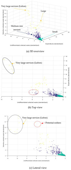
Figure 5.
Clusters obtained for Model A through the Ward’s method and the Euclidean distance.
However, from a simple inspection of plots provided therein, we concluded that the group of large observations could be detached into two: large and very large. In terms of standardized variables, very large observations were the ones “consuming” more than 10 (standard deviations of) money spent on MSW management. In fact, these very large observations corresponded to the eight observations of Lisbon city, the capital of Portugal. The displacement of this group from the remaining sample motivated the exclusion of this municipality (and its observations) from our further analysis. Furthermore, from (c) we can identify two potential outlier observations, collecting more than 10 (standard deviations of) quantity of selective waste. These cases were also removed from the sample.
Looking at (b), we observe a sub-cluster belonging to the medium size group, identified using a red dashed ellipsis. The difference between such a sub-cluster and the remaining cluster is considerable. Given that the former was composed of sixteen observations, we removed them from the sample. The cluster of large observations was also not large enough to produce efficiency results with good discrimination power. Hence, these were removed as well.
That being said, the efficiency analysis for Model A was based entirely on small- and medium-size observations, i.e., those simultaneously consuming less than 4 (standard deviations of) expenditures on MSW management and collecting less than 4 (standard deviations of both) refuse and selective waste.
In the same vein, and regarding the Model B, we investigated the existence of potential outliers and groups of observations composed of observations with distinct profiles in terms of waste. In this case, we considered five clusters, the Ward’s method and the Euclidean distance for the linkage, as shown in Figure 6. Using the same arguments as before, we retained only the services whose expenditures and landfilled waste were both below 4 and whose recycled waste was below 5 (standard deviations).
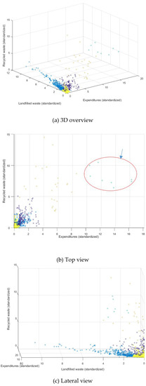
Figure 6.
Clusters obtained for Model B through the Ward’s method and the Euclidean distance.
Figure 7 exhibits the histograms and the most appropriate probability density functions (PDF) associated with the Portuguese MSW services’ economic efficiency. PDFs were selected based on the chi-square test for goodness of fit.
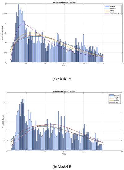
Figure 7.
Histograms and the most appropriate probability density functions associated with the Portuguese Municipal Solid Waste (MSW) services’ economic efficiency.
Regarding Model A, one can see that both the Birnbaum–Sanders and Weibull distributions were good approximations for the economic efficiency. We recall the results of Park et al. [43], Cazals et al. [38], and Daouia and Simar [44,45], who verified that the efficiency obtained through FDH and the partial frontiers (with α 1 or m ) asymptotically follow a Weibull distribution, although with unknown parameters. In this case,
with the scale parameter and the shape parameter. As usual, is the standard Gaussian distribution. Using the estimated parameters, we computed the expected average, , the expected standard deviation, , and the skewness, . These values compared with the observed ones: and . As for the case of the Weibull distribution, we had:
for which the scale parameter is and the shape parameter is . Accordingly, the expected average was , the standard deviation was , and the skewness was . Note that the Weibull distribution resulted in expected descriptive indicators (mean and standard deviation) that were closer to the observed ones than the Birnbaum–Sanders.
Considering Model B, the Weibull distribution fit the economic efficiency PDF well. Parameters were (scale) and (shape), resulting in (average), (standard deviation), and (skewness). In practice, (which is equal to ) and (very close to ).
Based on these findings and looking at Figure 7, the heterogeneity in our sample either in terms of scale size or the economic efficiency itself was considerable. Regarding the latter, the coefficient of variation was roughly 60%.
The most important outcome is perhaps the very low average economic efficiency in Portuguese MSW services. Based on the averages of efficiency distributions, , each service spent well 49% (= 100 × ) of its monetary resources to collect and treat MSW. The ANOVA technique resulted in F = 0.9871 and p = 0.7401, meaning that the average inefficiency levels remained nearly unchanged since 2010. Since the evaluated services consumed €3.5 billion on MSW between 2010 and 2017, each one squandered yearly €731 thousand, on average.
5.4. The Relationship between Economic Efficiency and the KPIs on MSW Management
Figure A1, Figure A2, Figure A3, Figure A4, Figure A5 and Figure A6 (Appendix A) exhibit the scatterplots relating the ratio for α = 0.50 (median frontier) or α = 1 (full frontier). The relationship between for α = 0.50 and the KPI allows the detection of the influence of the latter in the economic efficiency distribution. Contrarywise, if α = 1, then such a relationship identifies the factors impacting on best practices profiles.
To understand the relationship between the ratio and each one of the KPIs set, we considered a simple linear regression of the form for any KPI p = 1, …, 10 and for α = 0.5 or α = 1. This is a good fitting model provided that three conditions over residuals, , are met: homoskedasticity, independence, and normality, i.e., with and . The non-parametric Kolmogorov–Smirnov test concluded that residuals resulting from this linear relationship followed in general a Gaussian distribution with and . The Durbin–Watson test also concluded that residuals were independent. However, except for the tenth KPI, and according to the Breusch–Pagan test, residuals were heteroscedastic, as can be seen directly on Figure A1, Figure A2, Figure A3, Figure A4, Figure A5 and Figure A6. The linear regression model also exhibited very low coefficients of determination, nearly zero for most of them. This is mostly the result of a high heterogeneity on residuals. We additionally employed a Nadaraya–Watson non-parametric regression, but it also conduced to a trending line that was nearly constant all over the KPI domain. This results from the fact that residuals followed the standard normal distribution. Unfortunately, no other tested parametric regression had better outputs in terms of fitting.
The most relevant conclusion from the previous discussion is that , in general, is not dependent on the KPI itself, as the trending line seems to be nearly constant. For instance, the slope of the linear regression line, , was close to 0, while the intercept, , was always equal to 1. This indicates that the expected value of does not depend on the KPI value and it is unitary. Accordingly, the following was verified: for any j = 1, …, n, any p = 1, …, 10, and α = 0.5 or α = 1, where denotes the expected value. From Daraio and Simar [40], we know that both and can be formulated via the probability of observing the MSW service j dominating other observations within the sample. Putting it differently and recalling the Bayes’ theorem, we conclude that economic efficiency and performance indicators are, in general and statistically, independent from each other.
The major implication of these findings is that none of those KPIs can be used for performance assessment without hampering the outputs credibility. The reason is that these KPIs totally disregard important aspects of efficiency. Furthermore, unless a multicriteria decision analysis is undertaken to construct a composite based on KPIs, they do not account for regulatory and sustainability requirements. We do not criticize the utilization of KPIs in some basic regulatory actions, but making use of them as proxies or determinants for efficiency seems to be nonsense and founds no reason in empirical evidence. Claiming that MSW services spending more money per ton of collected waste are necessarily more inefficient is dangerous and should be avoided.
6. Discussion and Concluding Remarks
This study conducted an exploratory analysis to understand whether using some management-related KPIs instead of more robust benchmarking techniques brings similar outputs for regulators and MSW managers. Measuring the economic efficiency of MSW services is paramount for sustainability issues. In fact, we have verified that, on average and roughly speaking, half of expenditures with MSW services have been wasted simply because of inefficient practices. That huge level of inefficiency could be mitigated by searching for and adopting the best practices within the field of MSW management. In Portugal, only a few successful cases have been identified, as observed by the very low rate of economically efficient services (regardless of the adopted model).
It is worth mentioning that the adopted management-related KPIs, being just partial productivity measures, are incapable of identifying those best practices. Nor can they tell how far from the excellence the MSW service is, or at least in a segregated way. Even condensing KPIs into a single composite can be objectionable in some cases, provided the need for subjective (and, thus, likely biased) judgements. The individual analysis of KPIs has a limited and reduced value for regulation, although they continue to be extensively used for such purposes. This is probably because of their easy computation and interpretation. The MSW management system is multi-dimensional and, as was observed by Parekh [26], “the performance of some indicators is influenced by performance of other indicators like cost of transportation does not only depend on man power, machinery, spare vehicles but also depends on distance to landfill site, mode of operation i.e., departmental, contractual or Public Private Partnership mode”.
Bertanza et al. [33] argued that KPIs are not sufficient to explain economic efficiency, but they did not conduct an analysis more robust than simply measuring KPIs. A critique of past research is precisely the lack of comparison between KPIs and economic efficiency estimated through different ways. Our study, thus, comes to demystify the idea that KPIs can replace a more objective performance measurement, as the one obtained through the weight restricted order-α. None of the ten KPIs used were shown to be related to economic efficiency, nor did they explain the economic efficiency of MSW services or the best practices that belong to the efficient frontier. Therefore, those KPIs cannot be used instead of the economic/economic efficiency. This is in line with the claims of Bertanza et al. and constitutes an important result, as KPIs are used in the regulatory exercise. The main conclusion is not that KPIs should be disregarded totally from such an exercise. Rather, they should be complemented with other metrics, namely the efficiency estimates with weight restrictions, eventually giving more emphasis to the latter. In line with Ferreira et al. [46,47], these efficiency scores can be useful to adjust the price paid by the consumer for the collected waste, an exercise carried out by the regulator.
This study is not flawless. Some topics should be addressed in future research, namely the inclusion of other KPIs in the analysis. As shown in the literature revision, besides management there are other relevant categories that relate to efficiency, including the organizational and the governance levels that can be related to economic efficiency.
Author Contributions
All authors have contributed equally to this paper development. D.C.F. performed the experiments and wrote Section 4 and Section 5. R.C.M. designed the experiments (case study), wrote Section 1 and Section 6, reviewed and made substantial criticisms and changes on the entire manuscript. M.I.P. and C.A. collected and analyzed data and wrote Section 2 and Section 3. All authors have read and agreed to the published version of the manuscript.
Funding
This research received no external funding.
Acknowledgments
Any errors are the authors’ own responsibility. The usual disclaimer applies. The authors would like to thank to three anonymous referees who kindly and significantly have improved the paper’s quality, clarity, and structure, due to their beneficial comments.
Conflicts of Interest
The authors declare no conflict of interest.
Appendix A

Figure A1.
Scatterplots for the ratio Rα and KPIs 1 to 4, considering the full frontier.

Figure A2.
Scatterplots for the ratio Rα and KPIs 5 to 8, considering the full frontier.

Figure A3.
Scatterplots for the ratio Rα and KPIs 9 and 10, considering the full frontier.


Figure A4.
Scatterplots for the ratio Rα and KPIs 1 to 4, considering the median frontier (α = 0.50).


Figure A5.
Scatterplots for the ratio Rα and KPIs 5 to 8, considering the median frontier (α = 0.50).

Figure A6.
Scatterplots for the ratio Rα and KPIs 9 and 10, considering the median frontier (α = 0.50).
References
- Zaman, A. A comprehensive study of the environmental and economic benefits of resource recovery from global waste management systems. J. Clean. Prod. 2016, 124, 41–50. [Google Scholar] [CrossRef]
- Periathamby, A. Municipal Waste Management. In Waste: A Handbook for Management; Letcher, T.M., Vallero, D., Eds.; Academic Press: Boston, MA, USA, 2011; pp. 109–125. ISBN 978-0-12-381475-3. [Google Scholar]
- Tomic, T.; Schneider, D.R. Municipal solid waste system analysis through energy consumption and return approach. J. Env. Manag. 2017, 203, 973–987. [Google Scholar] [CrossRef]
- Carvalho, M. Optimização de circuitos e indicadores de recolha de resíduos urbanos. Caso de Estudo: Município de Almada. Ph.D. Thesis, University of Lisbon, Lisbon, Portugal, 2008. [Google Scholar]
- European Commission. Guidance on Municipal Waste Data Collection. Available online: https://ec.europa.eu/eurostat/documents/342366/351811/Municipal+Waste+guidance/bd38a449-7d30-44b6-a39f-8a20a9e67af2 (accessed on 3 February 2020).
- Rodrigues, S. Classificação e Benchmarking de Sistemas de Recolha de Resíduos Urbanos. Ph.D. Thesis, University of Lisbon, Lisbon, Portugal, 2016. [Google Scholar]
- Thomas, L. Managing municipal solid waste. J. Air Pollut. Control. Assoc. 1988, 38, 750–751. [Google Scholar]
- Chowdhury, M. Searching quality data for municipal solid waste planning. Waste Manag. 2009, 29, 2240–2247. [Google Scholar] [CrossRef]
- Simões, P.; Cavalho, P.; Marques, R.C. The market structure of urban solid waste services: How different models lead to different results. Local Gov. Stud. 2013, 39, 396–413. [Google Scholar] [CrossRef]
- Martinho, M.d.G. Factores determinantes para os comportamentos de reciclagem. Ph.D. Thesis, University of Lisbon, Lisbon, Portugal, 1998. [Google Scholar]
- Levy, J.; Cabeças, A. Resíduos Sólidos Urbanos—Princípios e Processos; AEPSA: Lisboa, Portugal, 2006. [Google Scholar]
- Shekdar, A.; Mistry, P. Evaluation of multifarious solid waste management systems—A goal programming approach. Waste Manag. Res. 2001, 19, 391–402. [Google Scholar] [CrossRef]
- Morgado, D. Strategic management of municipal solid waste in the Municipality of Alenquer: Application of the PAYT system. Master’s Thesis, University of Lisbon, Lisbon, Portugal, 2013. [Google Scholar]
- Marques, R.; Simões, P. Incentive regulation and performance measurement of the Portuguese solid waste management services. Waste Manag. Res. 2009, 27, 188–196. [Google Scholar] [CrossRef]
- Dias, A. Avaliação da Gestão de MSW a Nível Nacional—O Uso de Indicadores. Master’s Thesis, University of Aveiro, Aveiro, Portugal, 2009. [Google Scholar]
- Portuguese Environment Agency—PEMSW. Available online: http://archive.vn/qb6IK (accessed on 31 March 2020).
- Pemsw, I.I. Plano Estratégico para os Resíduos Sólidos Urbanos; Ministério do Ambiente do Ordenamento do Território e do Desenvolvimento Regional: Lisbon, Portugal, 2007; ISBN 9789898097019.
- Tchobanoglous, G.; Theisen, H.; Vigil, S. Integrated Solid Waste Management: Engineering Principles and Management Issues; McGraw-Hill: New York, NY, USA, 1993. [Google Scholar]
- McDougall, F.; White, P.; Franke, M.; Hindle, P. Integrated Solid Waste Management: A Life Cycle Inventory, 2nd ed.; Blackwell: Oxford, UK, 2001. [Google Scholar]
- ERSAR. Relatório Anual dos Serviços de Águas e Resíduos em Portugal; EPSAR: Valencia, Spain, 2018. [Google Scholar]
- ERSAR; LNEC. Guia de Avaliação da Qualidade dos Serviços de Águas e Resíduos Prestados aos Utilizadores; EPSAR: Valencia, Spain, 2019; Volume 3. [Google Scholar]
- Suttibak, S.; Nitivattananon, V. Assessment of factors influencing the performance of solid waste recycling programs. Resour. Conserv. Recycl. 2008, 53, 45–56. [Google Scholar] [CrossRef]
- Guimarães, B.; Simões, P.; Marques, R.C. Does performance evaluation help public managers? A Balanced Scorecard approach in urban waste services. J. Environ. Manag. 2010, 91, 2632–2638. [Google Scholar] [CrossRef]
- Mendes, P.; Santos, A.; Nunes, L.; Teixeira, M. Evaluating municipal solid waste management performance in regions with strong seasonal variability. Ecol. Indic. 2013, 30, 170–177. [Google Scholar] [CrossRef]
- Zaman, A. Identification of key assessment indicators of the zero waste management systems. Ecol. Indic. 2014, 36, 682–693. [Google Scholar] [CrossRef]
- Parekh, H.; Yadav, K.; Yadav, S.; Shah, N. Identification and assigning weight of indicator influencing performance of municipal solid waste management using AHP. KSCE J. Civ. Eng. 2015, 19, 36–45. [Google Scholar] [CrossRef]
- Teixeira, C.; Russo, M.; Matos, C.; Bentes, I. Evaluation of operational, economic, and environmental performance of mixed and selective collection of municipal solid waste: Porto case study. Waste Manag. Res. 2014, 32, 1210–1218. [Google Scholar] [CrossRef]
- Sanjeevi, V.; Shahabudeen, P. Development of performance indicators for municipal solid waste management (PIMS): A review. Waste Manag. Res. 2015, 33, 1052–1065. [Google Scholar] [CrossRef]
- Yang, W.; Lee, Y.; Hu, J. Urban sustainability assessment of Taiwan based on data envelopment analysis. Renew. Sustain. Energy Rev. 2016, 61, 341–353. [Google Scholar] [CrossRef]
- Martinho, G.; Gomes, A.; Santos, P.; Ramos, M.; Cardoso, J.; Silveira, A.; Pires, A. A case study of packaging waste collection systems in Portugal—Part I: Performance and operation analysis. Waste Manag. 2017, 61, 96–107. [Google Scholar] [CrossRef]
- Rodrigues, A.; Fernandes, M.; Rodrigues, M.; Bortoluzzi, S.; Gouvea da Costa, S.; Pinheiro de Lima, E. Developing criteria for performance assessment in municipal solid waste management. J. Clean. Prod. 2018, 186, 748–757. [Google Scholar] [CrossRef]
- Cetrulo, T.; Marques, R.C.; Cetrulo, N.; Pinto, F.; Moreira, R.; Mendizábal-Cortés, A.; Malheiros, T. Effectiveness of solid waste policies in developing countries: A case study in Brazil. J. Clean. Prod. 2018, 205, 179–187. [Google Scholar] [CrossRef]
- Bertanza, G.; Ziliani, E.; Menoni, L. Techno-economic performance indicators of municipal solid waste collection strategies. Waste Manag. 2018, 74, 86–97. [Google Scholar] [CrossRef]
- Deus, R.; Bezerra, B.; Battistelle, R. Solid waste indicators and their implications for management practice. Int. J. Environ. Sci. Technol. 2019, 16, 1129–1144. [Google Scholar] [CrossRef]
- Aragon, Y.; Daouia, A.; Thomas-Agnan, C. Nonparametric frontier estimation: A conditional quantile-based approach. Econ. Theory 2005, 21, 358–389. [Google Scholar] [CrossRef]
- Agrell, P.; Tind, J. A Dual Approach to Nonconvex Frontier Models. J. Product. Anal. 2001, 16, 129–147. [Google Scholar] [CrossRef]
- Ferreira, D.C.; Marques, R.C. A step forward on order-α robust nonparametric method: Inclusion of weight restrictions, convexity and non-variable returns to scale. Oper. Res. 2017, 20, 1011–1046. [Google Scholar] [CrossRef]
- Cazals, C.; Florens, J.; Simar, L. Nonparametric frontier estimation: A robust approach. J. Econ. 2002, 106, 1–25. [Google Scholar] [CrossRef]
- Daouia, A.; Gijbels, I. Robustness and inference in nonparametric partial frontier modeling. J. Econ. 2011, 161, 147–165. [Google Scholar] [CrossRef]
- Daraio, C.; Simar, L. Directional distances and their robust versions: Computational and testing issues. Eur. J. Oper. Res. 2014, 237, 358–369. [Google Scholar] [CrossRef]
- Badin, L.; Daraio, C.; Simar, L. How to measure the impact of environmental factors in a nonparametric production model. Eur. J. Oper. Res. 2012, 223, 818–833. [Google Scholar] [CrossRef]
- Caldas, P.; Ferreira, D.; Dollery, B.; Marques, R.C. Are there scale economies in urban waste and wastewater municipal services? A non-radial input-oriented model applied to the Portuguese local government. J. Clean. Prod. 2019, 219, 531–539. [Google Scholar] [CrossRef]
- Park, B.; Simar, L.; Weiner, C. The FDH estimator for productivity efficiency scores: Asymptotic properties. Econ. Theory 2000, 16, 855–877. [Google Scholar] [CrossRef]
- Daouia, A.; Simar, L. Robust nonparametric estimators of monotone boundaries. J. Multivar. Anal. 2005, 96, 311–331. [Google Scholar] [CrossRef][Green Version]
- Daouia, A.; Simar, L. Nonparametric efficiency analysis: A multivariate conditional quantile approach. J. Econ. 2007, 140, 375–400. [Google Scholar] [CrossRef]
- Ferreira, D.C.; Marques, R.C.; Nunes, A.M. Pay for performance in health care: A new best practice tariff-based tool using a log-linear piecewise frontier function and a dual–primal approach for unique solutions. Oper. Res. 2019. [Google Scholar] [CrossRef]
- Ferreira, D.C.; Nunes, A.M.; Marques, R.C. Optimizing payments based on efficiency, quality, complexity, and heterogeneity: The case of hospital funding. Int. Trans. Oper. Res. 2020, 27, 1930–1961. [Google Scholar] [CrossRef]
© 2020 by the authors. Licensee MDPI, Basel, Switzerland. This article is an open access article distributed under the terms and conditions of the Creative Commons Attribution (CC BY) license (http://creativecommons.org/licenses/by/4.0/).