Operating Times and Users’ Behavior at Urban Road Intersections

Abstract

The safety of at grade road intersections is a relevant issue with social, economic, and environmental implications. It is related to the behavior of a driver approaching an intersection that, in its turn, is affected by kinematic and physiological variables. This study proposes a model to calculate the intersection operation time (IOT) for typical non-signalized 4-leg and 3-leg (or T-leg) urban intersections. Data available in the literature have been considered in order to identify the points of interest and assess the number and the time of a driver’s eye fixation on them. When approaching an intersection, the probability of glancing in a particular area changes with the distance to the yield or stop line; for this reason, a probabilistic approach was used to model the phenomenon. All possible maneuvers have been considered: left turning, right turning, and through-movement. The proposed model allowed an objective comparison between time spent by drivers for various maneuvers and layout conditions, and identification of the critical conditions. Indeed, significant differences in terms of IOT were found: they could lead to modification of the traffic management considering different needs of road users, traffic demand, and geometrical and functional constraints.

1. Introduction

An at-grade intersection is the area shared by two or more roads that join or cross each other [1]. Therefore, at intersections vehicles make maneuvers: they end the almost constant-speed conditions and low-curvature trajectories to pass to an unsteady motion state [2]. Generally, left turn, right turn, and straight-through movement are the allowable maneuvers: each vehicle makes a set of operations, speed, and direction changes to set and follow its flow trajectory. Safety and efficiency are the two-conflicting parameters commonly adopted to design, describe, model, and predict the intersection performance [3]. High portion of total crashes occurs at intersections, especially in the urban environment where drivers, pedestrians, and cyclists interact in shared spaces under time pressure [4,5,6].

The intersection operation time (IOT) is the time duration of a vehicle on a specific intersection from the approach to the complete execution of the maneuver: it is composed of approaching, waiting, and decision times. The time spent by drivers at intersection depends on the geometric features of the intersection and the relationship between himself, the infrastructure, and the surrounding traffic environment. The controller of the system is the driver him/herself: he/she must analyze the intersection area (and the evolving scenario) while approaching it and change his/her movements according to the surrounding environment, in order to perform the operation needed to complete the maneuver. They collect sight and hearing outside input data and afterwards make a decision; during this time, drivers have to avoid collision with other vehicles or road users. The more scenario complexity there is, the more time is needed to analyze it; the number of lanes, visual obstructions, and different user categories make the scenario hard to interpret. Therefore, IOT is a crucial parameter for measuring the intersection efficiency [7].

In the literature, several studies tried to analytically model the drivers’ behavior during the approaching phase, because it reflects the relationship between the driver and the surrounding environment. In the last years, studies of driver’s eye-scanning investigated the influence of road alignment during their approaching time [8,9]. Eye-tracking equipment was used to monitor the drivers’ visual search patterns; eye movements were recorded using a head-mounted eye-tracking device [10]. Three categories of data are most frequently considered: what the users scan [11]; the number of fixations [12]; how long the users scan [13]. Moreover, the visual behavior depends on the presence of signals at an intersection [14], the maneuver that drivers made [15], the time of the day [16], the surrounding objects [17], the driver’s experience [18], and the lighting conditions [19]. Since eye movement and steering are linked, because the driver’s choices stem from their visual information [20], these data contribute to modeling the driver’s behavior when approaching an intersection.

In contrast to the approaching time, the relationship between the user and infrastructure does not affect waiting and turning times. Instead, waiting time depends on the possibility of finding a Gap greater than Gap acceptance (i.e., the time interval between two consecutive vehicles evaluated by a driver for a crossing or merging operation), while the turning time depends on the length of maneuver and the vehicle type [1]. In the literature, the Gap acceptance processes have been analyzed in order to identify which variables influence the identification of an adequate opportunity to start a maneuver (e.g., individual drivers’ preferences, vehicle distance [21,22]). Microscopic simulation models and tools have been often used for approaching the analysis of drivers’ behavior for some special road configuration or traffic conditions [23,24,25].

The aim of this paper is to propose an analytical model to calculate IOT for urban at-grade road intersections, considering the different phases of admitted maneuvers and the time needed for the analysis, decision, and operation performed by drivers. Two geometrical layouts of three-leg (3-leg, T-type, or T-leg intersection) and four-leg (4-leg) urban intersections were considered. In all the examined cases, vehicles can perform three maneuvers: crossing (through-movement), right turn, and left turn.

2. Methods

Whatever the studied maneuver, IOT can be defined according to Equation (1):

IOT = t_MAN + t_REA

(1)

where t_MAN is the maneuver time: it is the time necessary to start and conclude the maneuver, and t_REA is the reaction time: it is the total time needed for a driver to perceive, decide, and react to an event on the road when a driver has to restart at the stop bar [26].

In order to model IOT, t_MAN was divided into three consecutive periods (Equation (2)):

• the approaching time (t_APP) in which a driver arrives on the threshold of intersection;
• the waiting time (t_WAI) in which a driver waits for an acceptable length of time on principal flow;
• the turning time (t_TUR) in which a driver carries out the maneuver.

IOT = t_APP+ t_WAI + t_TUR + t_REA.

(2)

2.1. Approaching Time

In this study, the approaching maneuver has been modeled as follows.

During t_APP, the driver travels along the road stretch L, which is the approaching leg: it starts from the road section when the driver perceives the intersection moving at the speed V_A and ends at the stop (or yield) bar. According to the Italian standard for road design [27] and the common layouts for road signaling at intersections, L is assumed to be equal to 150 m.

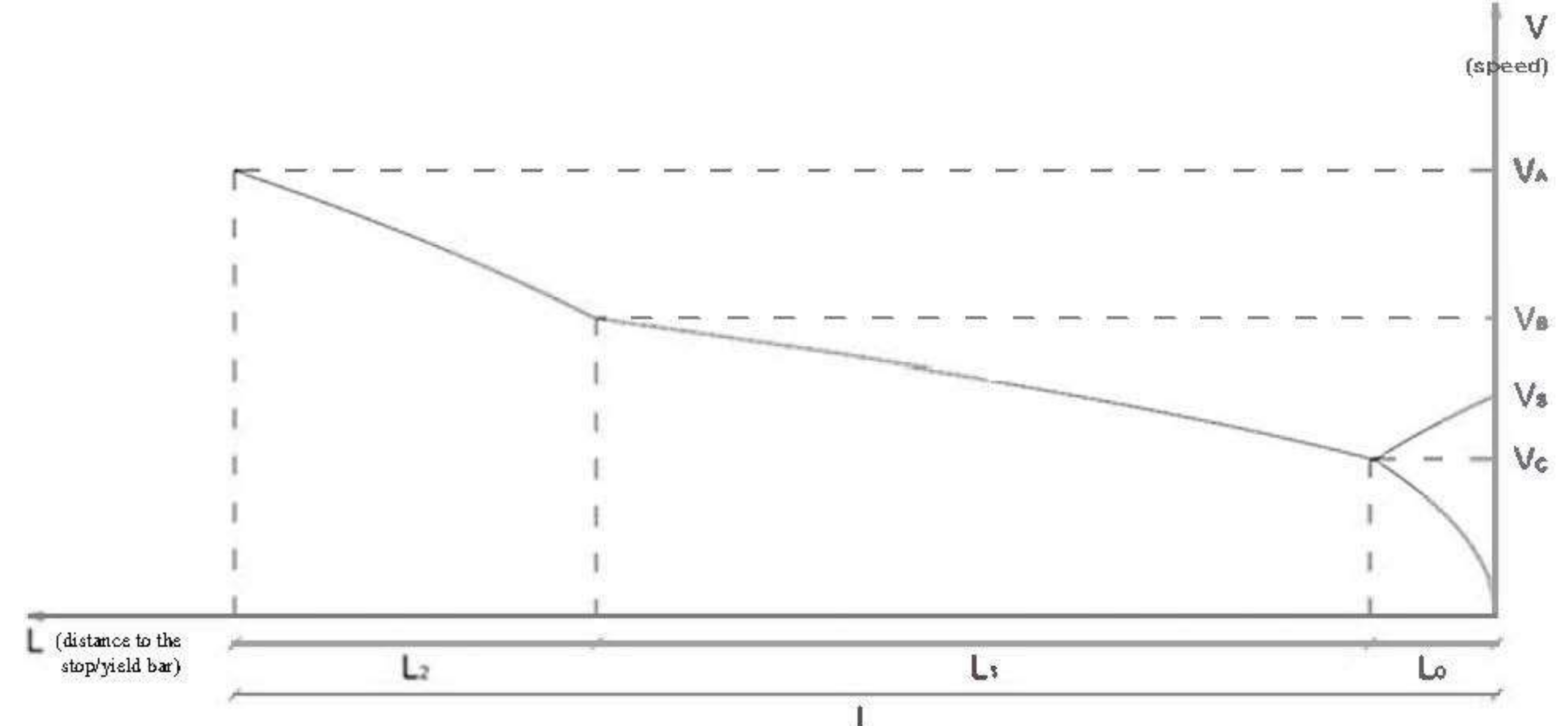
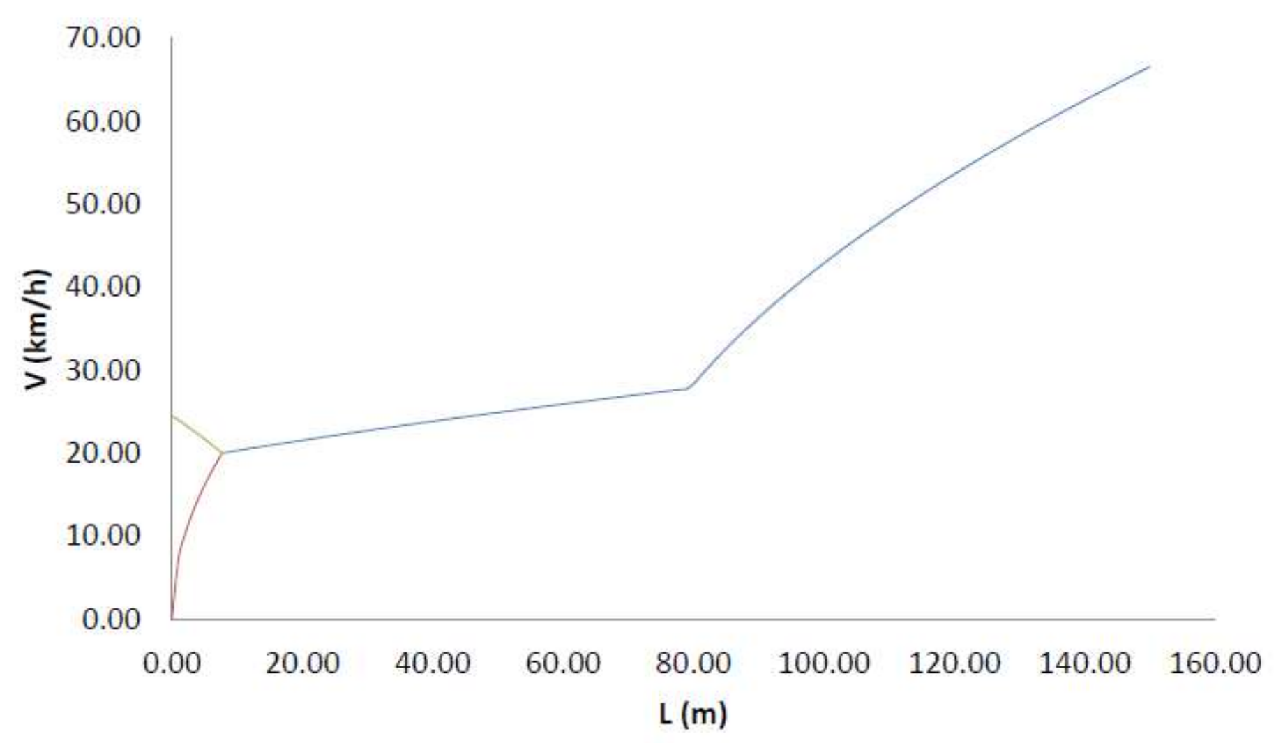
L is composed by different dynamic conditions along its three subsections (Figure 1):

• in the subsection (L₂), the driver decelerates from the current design speed (V_A) using the braking system until reaching V_B;
• in the ensuing subsection (L₁), the driver starts to analyze the other traffic flow to identify a possible acceptable gap. In this phase, the driver does not use the braking system until he reaches the decision point at the speed V_C;
• in the last subsection (L₀), two options are available. The driver can stop the vehicle at the stop bar or he can find an acceptable gap to maneuver without stopping the vehicle (i.e., a continuous maneuver) at the yield bar.

According to the principle of kinetic energy conservation and the rule of uniformly accelerated motion, Equations (3) to (8) can be used to describe the process.

L₂ = (V_A² − V_B²) / (2 d₂)

(3)

L₁ = (V_B² − V_C²) / (2 d₁)

(4)

L₀ = V_C² / (2 d₀)

(5)

L₁ = L₂ + L₁ + L₀ = (V_A² − V_B²) / (2 d₂) + (V_B² − V_C²) / (2 d₁) + V_C² / (2 d₀)

(6)

V_B = ((2 d₀ d₁ d₂ L − V_A² d₀ d₁ − V_C² d₂ (d₁ − d₀)) / (d₀ (d₂ − d₁))^0.5

(7)

V_S = (V_C² + 2 a L₀)

(8)

where a is the acceleration from V_C to V_S; V_C is assumed to be equal to 20 km/h; V_S is the threshold speed of the vehicle when it does not stop at the intersection and starts its maneuver at the speed V_S; d₀, d₁, and d₂ are the constant deceleration values along subsections L₀, L₁, and L₂, respectively. Deceleration values can be obtained through experimental observation. However, d₁ satisfies Equation (9) to have reasonable results:

d₁ ≤ d_1,max = (V_A² − V_C²) / (2 (L − L₀))

(9)

where d_1,max is the maximum reasonable value of d₁: it occurs when the driver starts uniformly decelerating from V_A to V_C when he is at a distance L from the stop line.

Given Equations (3) to (8), it is possible to calculate the time spent by the driver along L₀, L₁, and L₂. The approaching time values for stopping and continuous maneuvers are t_APP,0 and t_APP,S (Equations (10) and (11), respectively).

t_APP,0 = t₀ + t₁ + t₂

(10)

t_APP,S = t_S + t₁ + t₂.

(11)

According to [11], the driver’s behavior could be described by the time he spends to analyze a scenario. When approaching an intersection, the vehicle moves in unsteady conditions: for this reason, the approaching leg L should be divided into N dx-long branches (dx_i) (Equation (12)).

L = Σ_i^N dx_i = N dx

(12)

The discretization of L permits us to study the variation of eye’s fixation points varying the distance to the stop (or yield) bar. The driver’s fixations are affected by the presence (or absence) of some points of interest. In this study, 9 of them were considered:

• A traffic light for crossing or turning-right vehicles;
• A traffic light for turning-left vehicles when a dedicated turning lane is present;
• Traffic coming from the left;
• Traffic coming from the right;
• Traffic coming from the opposite direction (for 4-leg intersection);
• Pedestrian crossing on the left side of the approaching leg;
• Pedestrian crossing on the right side of the approaching leg;
• Vehicles on the left of the driver;
• Vehicles on the right of the driver.

Having regard to a group of m drivers, each k-th point of interest [traffic element] along the i-th branch is characterized by the average fixation time on it t_d,k,i and the number of total fixations made by drivers on it f_T,k,i. Therefore, Equation (13) gives the overall average time t_f,d,i that a driver spends to analyze the i-th dx_i:

t_f,d,i = M t_s + Σ_k=1^M (α f_T,k,i t_d,k,i) / M

(13)

where M is the number of focused points of interest along dx_i and t_s is the time of saccade (i.e., small rapid jerky movement of the eye when it jumps from fixation on one point to another). In this study, t_s has been assumed equal to 225 ms [28]; α is the percentile of risk propensity of a driver (considered as a representative of the average of driver population). This value describes the probability value that simulates a driver’s risk appetite (risk propensity).

Equation (14) gives the average time spent by drivers to analyze the approaching leg t_d,a:

t_d,a = Σ_i=1^N t_f,d,i / N.

(14)

Given t_d,a, it is possible to calculate the average speed V_d that a driver has to maintain to analyze L in safety conditions (Equation (15)). In this study, V_d is the value assumed for V_A because it ensures the safety condition described herein.

V_d = L / t_d,a

(15)

The comparison between t_d,a and t_APP,0 or t_APP,S gives the conditions (Equations (16) to (19)):

• when

t_d,a ≤ t_APP,0

(16)

t_d,a ≤ t_APP,S.

(17)

The driver can analyze the scenario in safety conditions. This result is acceptable.

• when

t_d,a > t_APP,0

(18)

t_d,a > t_APP,S.

(19)

The driver cannot analyze the scenario under safety conditions because V_d is smaller than the travel speed. This condition is not acceptable: since the driver cannot analyze the intersection under safety conditions, he has to reduce his travel speed to approach safely the intersection.

Having regard to the continuous maneuver (Equation (11)), Equation (20) describes the time spent by a driver to evaluate the possibility of a continuous maneuver being needed:

T > t₁ + t_S.

(20)

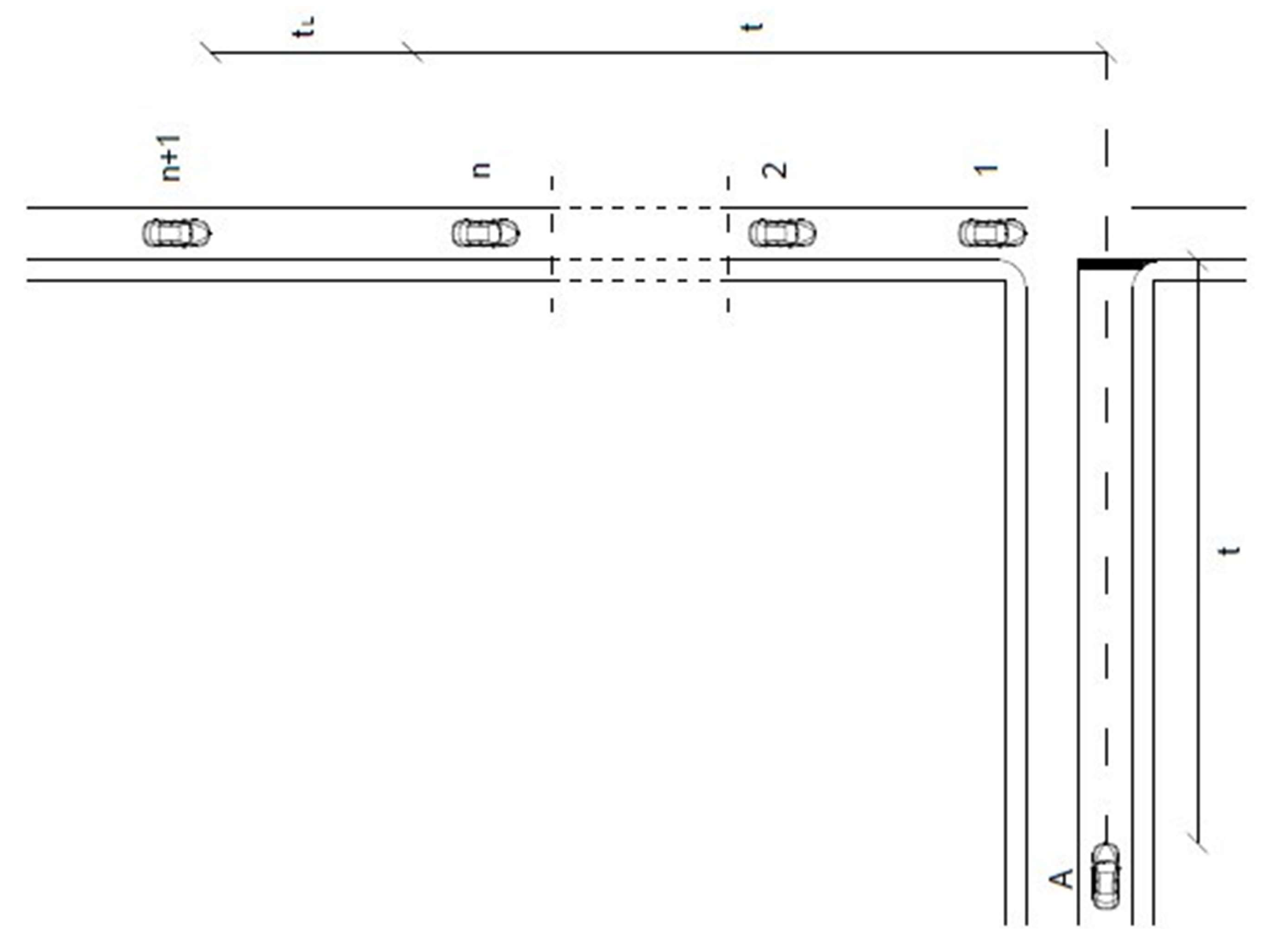
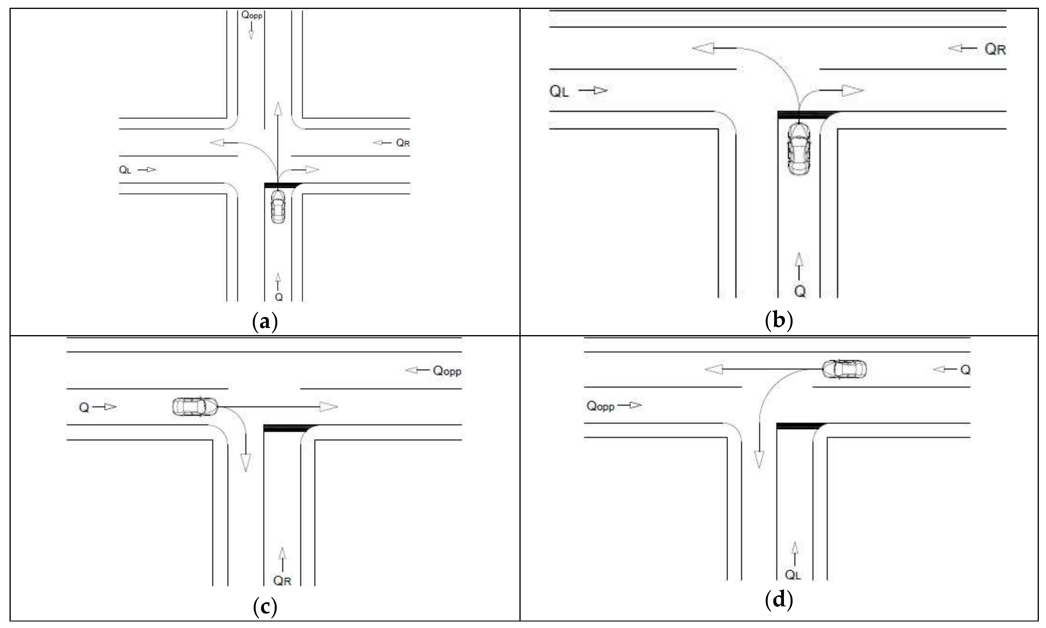
In Equation (20) t₂ is not considered because the driver starts to analyze the other traffic flows when he is at the point B (Figure 1). In order to describe the process, the proposed probabilistic model considers that when a vehicle (vehicle A in Figure 2) is arriving at the yield bar (during T), v vehicles pass along the perpendicular flow. Therefore, the Poisson distribution could describe the process (Equation (21)):

$$P(x=v)=\frac{{\mu }^x}{x!}·e^{-\mu }=\frac{{\left(Q·T\right)}^x}{x!}·e^{-\left(Q·T\right)}$$

(21)

where μ is the average number of vehicles that pass the intersection during T and Q is the traffic flow of perpendicular lanes.

Given T and Q, it is necessary to establish a percentile Plim in order to find the (entire) number of vehicles (v) such that the probability v vehicles pass the intersection during T is equal or more than Plim (Equation (22)):

P(x = v) ≥ Plim.

(22)

When the v-th vehicle has passed the intersection, the time between the passing of vehicle v and vehicle v+1 is the available lap (t_L) for the approaching driver. Therefore, Equation (23) is valid and allows us to obtain t_L:

$$P\left(x=v|T\right)=P\left(x=v+1|T+t_L\right)=\frac{{\left[Q·\left(t+t_L\right)\right]}^{v+1}}{\left(v+1\right)!}·e^{-Q·\left(t+t_L\right)}.$$

(23)

The comparison between t_L and the lap acceptance (t_LAP,A) identifies two conditions (Equations (24) and (25)):

t_L ≥ t_LAP,A.

(24)

The continuous maneuver is possible: the approaching time is t_APP,S; or

t_L < t_LAP,A.

(25)

The driver has to arrest a vehicle on the yield bar: the approaching time is t_APP,0.

2.2. Waiting Time

When Equation (25) is satisfied, or the driver stops his vehicle at the stop bar, he has to find an available gap τ that is not less than the gap acceptance t_GAP,A (Equation (26)):

τ ≥ t_GAP,A.

(26)

This study proposed a model to describe how much time a driver needs to wait for on the stop (or yield) bar to find an available gap on the principal traffic flow. Probabilistic laws describe the distribution of vehicle spacing in a traffic flow [21] in order to find the number of vehicular spacing that satisfy Equation (26). Equation (27) gives the number of suitable vehicular spacing for entry maneuver (q_i) when the exceedance probability P(τ ≥ t_GAP,A) and q are multiplied (Equation (28)):

$${\mathit{q}}_{\mathit{i}}=\mathit{q}\mathit{P}(\tau \ge {\mathit{t}}_{\mathit{GAP},\mathit{A}})=\frac{Q-1}{3600}·P\left(\tau \ge t_{GAP,A}\right)$$

(27)

where Q is the traffic flow in km/h, q is the number of vehicular spacing in 1 s.

Under steady flow conditions, the Poisson distribution is suitable for describing the phenomenon of a single traffic stream. In such conditions, Equation (28) describes the number of suitable spacings (ξ) during τ.

ξ = q_i τ

(28)

Equation (29) gives the percentile value when no enough vehicular spacing happens (ξ=0) during τ (i.e., the waiting time):

$$P\left(\xi =0\right)=\frac{{\left(q_i·\tau \right)}^0}{0!}·e^{-q_i·\tau }=e^{-q_i·\tau }$$

(29)

P(ξ = 0) has been assumed to be equal to 0.8. However, the exponential curve gives not-null probability values for tending to zero time values; it is an impossible condition due to the finite length of vehicles. Therefore, a shifted exponential distribution proposed by [29] has been considered (Equations (30) and (31)):

f(τ) = 0 when τ < c

(30)

$$f(·)=\frac{1}{\frac{1}{\lambda }-c}{e}^{\left(-\frac{\tau -c}{\frac{1}{\lambda }-c}\right)}\mathrm{when}\tau \ge c$$

(31)

where c is the lowest vehicular spacing for a given Q value (e.g., 0.5–1 s according to [3]), and λ is assumed to be the reciprocal of Q.

2.3. Turning Time

Turning time (t_TUR) can be obtained by analyzing vehicular movements and speed during each maneuver at an intersection. In this study, by means of a statistical treatment, it was possible to define the average maneuver speed V_a. Then, for each maneuver when knowing its length (Z), Equation (32) gives t_TUR for horizontal approaching legs:

t_TUR = Z / V_a.

(32)

2.4. Data from the Literature

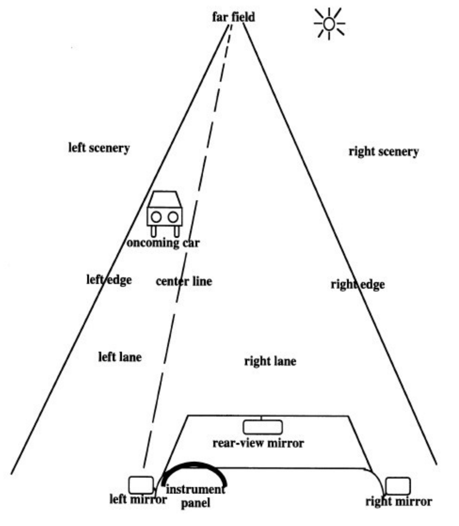
The proposed methodology has been implemented by using some parameters obtained from the literature, especially with regard to the data that could not be deduced from theoretical models or directly obtained from experimental surveys. This opportunity especially concerns the data regarding fixation parameters, that are available in the literature. Particularly, Colleen [12] analyzed the fixation areas during the day (Figure 3). She divided straight road sections into several zones (i.e., far field, right scenery, and left scenery) composed of different fields.

For a 106.68 m-long straight section, it was possible to calculate the time of fixations towards each field in Figure 3 and obtain its fixation times. According to Equation (15), the sum of all fixation times and the length of the examined section allowed calculation of V_d (i.e., the average speed along a straight section): in this study V_d and V_A are 66.56 km/h.

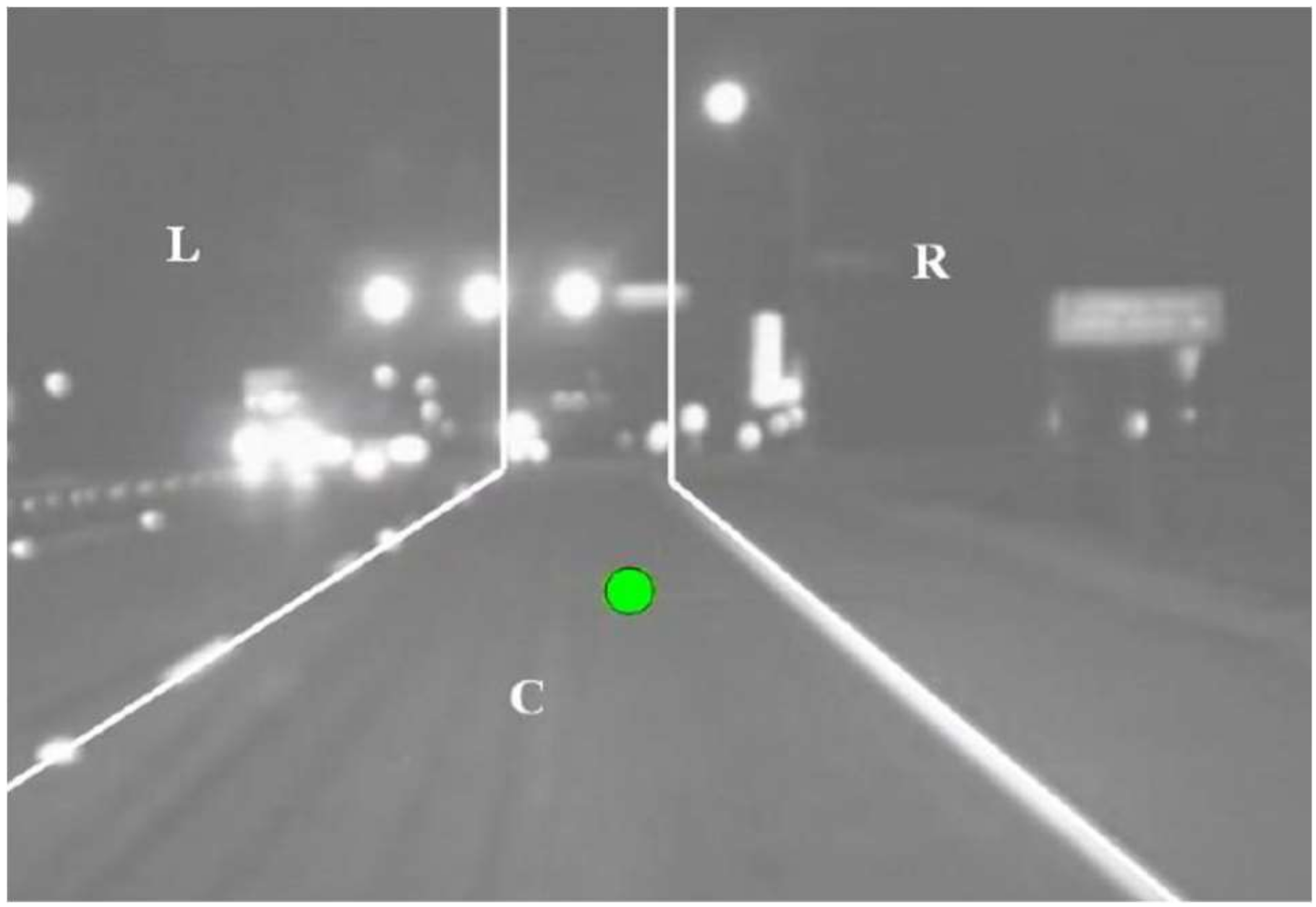
On the other hand, two studies conducted by Higgins [13,15] on the number and duration of fixations, and the points focused by drivers approaching a road intersection were considered. Higgins [15] divided the scenario approaching unsignalized intersections into 4 glance areas (Figure 4):

• left (L): this includes all lanes and objects on the left of the driver (i.e., left hand side pedestrians, left adjacent traffic, and left path of travel);
• center (C): this includes the lane where the driver is moving and all frontal elements (i.e., adjacent to the signal and opposing traffic);
• right (R): this includes all lanes and objects on the right of the driver (i.e., right adjacent traffic, right hand side pedestrians, and right path of travel);
• off screen (O): this covers all zones not included in the examined glance areas.

For each area, at a different distance from the stop or yield bar, the number and duration of glances were considered. Having regard to [11] and [13,15], a binary logistic regression model was adopted to describe the probability of a fixation, in a given glance area. The results from the statistical analysis allowed calculation of the average fixation duration and the average number of fixations for each glance area and considered maneuver (i.e., right turn, through, and left turn) in the examined intersections (

Table 1. Average fixation durations and number of fixations.

Maneuver	Average Fixation Duration (s)
	L	C	R	O
Right turn	0.85	0.50	1.10	0.50
Through	0.53	0.57	1.00	0.50
Left turn	0.80	0.40	0.60	0.50
Maneuver	Average Number of Fixations
	L	C	R	O
Right turn	1.04	2.53	5.49	0.62
Through	0.80	2.48	4.11	0.57
Left turn	1.27	3.02	8.26	0.73

).

3. Results

The fixation model has been implemented to analyze two intersections in the Southern Italy: a 4-leg intersection in Molfetta (BA) (Figure 5a) (I1) and a T-leg intersection in Bari-porto (BA) (Figure 5b) (I2).

For each configuration in Figure 5, three functional cases have been examined: three maneuvers in the 4-leg intersection (Figure 6a) and three scenarios in the T-type intersection (Figure 6b–d). In this paper, the 4-leg intersection is named X1, while the T-leg scenarios in Figure 6b–d is named as T1, T2, and T3, respectively.

According to Figure 6,

Table 2. Traffic flow input data.

Traffic Volume	Value (veh./h)
QL	600
QR	600
Qopp	400

lists the traffic flow input data that were collected during 15 min-long traffic counts according to the Highway Capacity Manual [30]; data from different days and hours has been used. The surveys were conducted in October, when the weather condition is not an obstacle to trips and all work- and school-related activities are ongoing.

Table 3. Kinematic input data.

Variable	Value	Unit
d0	2	m/s2
d1	0.2	m/s2
d2	2	m/s2
a	1	m/s2
α	0.80	-

lists the values of d₀, d₁, d₂, a, and α. d₀, d₂, and a comply with the Italian standard for road design [31]; for d₁ the authors assumed a small value because in L₁ the driver does not use the braking system and the vehicle speed is almost constant. α has to be assumed as a percentile value (in this study, it is equal to 0.8).

According to Equations (3) to (8), Figure 7 shows the calculated speed curve along L (V_A, V_B, and V_V are 66.56 km/h, 27.78 km/h, and 24.49 km/h, respectively):

• the blue curve represents the cinematic trend along L₂ and L₁;
• the red curve represents the speed trend when Equation (25) is satisfied;
• the green curve describes the speed trend when Equation (24) is satisfied.

Therefore,

Table 4. Approaching times.

Time	Value (s)
tAPP,0	18.97
tAPP,S	17.44
t0	2.78
t1	10.80
t2	5.39
tS	1.25

lists the overall approaching times t_APP,0 and t_APP,S and their partial values along the subsections L₀, L₁, and L₂.

According to Equation (20), T is equal to 12.05 s.

Video records provided by TPS Transport Planning Service allowed the data collection in order to determine maneuver times.

Table 5. t_d,a values.

Scenario	X1	T1	T2	T3
Maneuver	td,a (s)
Right Turn	8.48	7.31	7.66	-
Through	5.71	-	5.24	2.17
Left Turn	7.93	5.50	-	2.58

lists the average time spent by drivers to analyze the intersections, maintaining an adequate safety degree.

According to Table 5, all t_d,a values are not more than t_APP,0 and t_APP,S (Equations (16) and (17)): the driver can analyze the scenario in safety conditions, but the continuous maneuvers should be verified. At this purpose, in the T-type intersection, the right of way has been considered. Therefore, all maneuvers in T2 and the through maneuver in T3 have not been analyzed for calculation of t_L.

Table 6. t_L values.

Scenario	X1	T1	T2	T3
Maneuver	tL (s)
Right Turn	4.44	4.44	not analyzed	-
Through	2.33	-	not analyzed	not analyzed
Left Turn	6.37	2.33	-	6.42

lists the t_L values obtained from Equations (24) and (25), having Plim equal to 80%.

These values have been compared with the t_LAP,A that is assumed to be equal to 6.36 s on the basis of the LAP/GAP ratio observed in the performed surveys and having regard to [22]. Therefore, all t_L values in X1 and T1 (Table 6) satisfy Equation (25) and the continuous maneuver is not possible; on the contrary, in T3 the continuous left turn is possible.

In order to calculate t_WAI, t_GAP,A has been derived from [32] and assumed equal to 7.87 s according to [22]. Equations (30) and (31) allow the analysis of the vehicular spacing:

Table 7. Exceedance probability values.

Scenario	X1	T1	T2	T3
Maneuver	P(τ ≥ tGAP,A)
Right Turn	0.28	0.28	not analyzed	-
Through	0.04	-	not analyzed	not analyzed
Left Turn	0.02	0.04	-	0.43

and

Table 8. t_WAI values.

Scenario	X1	T1	T2	T3
Maneuver	tWAI (s)
Right Turn	4.78	4.78	not analyzed	-
Through	35.60	-	not analyzed	not analyzed
Left Turn	49.81	35.60	-	4.70

list the obtained P(τ ≥ t_GAP,A) and t_WAI, respectively.

Given the geometrical layout of I1 and I2, the maneuver lengths are in

Table 9. Maneuver lengths.

Scenario	X1	T1	T2	T3
Maneuver	Z (m)
Right Turn	4.50	4.50	4.50	-
Through	9.50	-	9.50	9.50
Left Turn	10.50	10.50	-	10.50

.

Having regard to the measured speed V_a and the trajectory lengths in Table 9,

Table 10. Turning times.

Scenario	X1	T1	T2	T3
Maneuver	tTUR (s)
Right Turn	1.50	1.50	1.10	-
Through	1.48	-	0.88	0.88
Left Turn	2.14	2.14	-	1.70

lists the obtained t_TUR values.

Finally, according to Equation (2) and given t_REA equal to 2 s [31],

Table 11. IOT time.

Scenario	X1	T1	T2	T3
Maneuver	IOT (s)
Right Turn	27.18	27.18	18.54	-
Through	28.05	-	18.32	18.32
Left Turn	72.92	58.71	-	19.14

lists the IOT values.

4. Discussion

The time spent by a driver when he is approaching a road intersection depends on two variables: the first one is a kinematic problem, while the second one is a physiological factor. The correlation between these two variables affects the time that a driver has to spend approaching safely an intersection. The proposed model combines these two aspects joining the literature experience with video records in order to calculate the intersection operation time for two scenarios: a 4-leg intersection and a T-leg intersection. Particularly, IOT is composed of the reaction time, approaching time, waiting time, and turning time.

The comparison between the approaching time calculated with a kinematic approach and the average time spent by drivers to analyze the approaching leg satisfies all the examined scenarios in Equation (33):

t_d,a ≤ t_APP.

(33)

Therefore, safety conditions are ensured in the analyzed intersections. However, the stop bar or the presence of traffic flow in other directions could prevent the continuous maneuver and the vehicles should stop and wait at the yield bar. Having regard to the waiting time, the obtained results confirm an expectable trend: lower waiting times are typical of simple maneuvers, while larger waiting times are characteristics of complex ones. Overall, the obtained results are realistic: the greater the intersection complexity, the higher the intersection operation time needed. Indeed, for each modeled maneuver, I2 has lower or equal IOT compared to I1.

However, the hypotheses put forward by the authors cannot be overlooked: the obtained results are affected by the cited documents and the proposed calibration procedures. In order to guarantee the reliability of results, experimental campaigns for data collection shall be specifically designed for the studied problem. Indeed, road intersections could have variable layouts (e.g., geometry configuration, surrounding elements) that affect behavior. Therefore, each different layout influences the glance distribution in space and in time. The eye-fixations analysis was not conducted to evaluate waiting time, turning time, and reaction time because the main features that influence time on intersection are the number of vehicles in principal flow, the geometric features of intersection, and the type of vehicle.

5. Conclusions

The purpose of this study was to define a methodology to model a driver’s behavior during approaching and turning phases at on-grade road intersections. Comparing operating times depending on the type of the maneuver, it is possible to observe greater times for turning left and lower ones for turning right. This is not true for T-type intersections in case 2 and case 3 where operating time values are similar. This is due to the fact that the vehicle in this case makes a continuous maneuver without waiting on the stop bar. Comparing operating times depending on the type of intersection, it is possible to observe that T-type intersections present lower values of operating time, especially when continuous maneuvers are possible. Furthermore, it was underlined how the driver-infrastructure-environment interaction is an important element used to study safety behaviors during the approach and turning maneuvers. Even if the calibration brought low values of the analysis times, it was observed that increasing complexity and elements of the intersections increase these times that become binding for the model. For this reason, it is possible to assert that the model can be seen as a useful instrument to better understand the mechanisms that underlie the accomplishment of maneuvers in order to perfect the design tools. Policy and decision makers could apply it when they have to manage urban road safety because it provides results that could be used to critically approach this strategic sector whose impacts are economic, social, and environmental. Indeed, input data are available to a road management body, and the presented method is comprehensive and versatile; therefore, it may be applied to different urban scenarios by varying the examined variables and their factors. Future development prospects involve validating the model through microsimulation and experimental field observations.

The model presents some validation limits. The results shown in this report are affected by some calibration problems that could influence their reliability. To show the reliability of the results, the experimental methods for data collection should be specifically designed for the case study. Furthermore, intersections present different elements and characteristics that could not be always present. In the calibration, the not present elements were simply delated from fixation analysis. This process has some errors because the absence of an element involves a redistribution of fixations.

References

1. Gerlough, D.L.; Huber, M.J. Traffic Flow Theory; Special Report 165; Transportation Research Board, National Research Council: Washington, DC, USA, 1975. [Google Scholar]
2. Maerivoet, S.; De Moor, B. Traffic flow theory. arXiv 2005, arXiv:physics/0507126. Available online: https://arxiv.org/abs/physics/0507126 (accessed on 15 May 2020).
3. Gartner, N.H.; Messer, C.J.; Rathi, A. Traffic Flow Theory-A State-of-the-Art Report: Revised Monograph on Traffic Flow Theory. 2002. Available online: https://rosap.ntl.bts.gov/view/dot/35775 (accessed on 15 May 2020).
4. Dogan, E.; Steg, L.; Delhomme, P. The influence of multiple goals on driving behavior: The case of safety, time saving, and fuel saving. Accid. Anal. Prev. 2011, 43, 1635–1643. [Google Scholar] [CrossRef] [PubMed]
5. Cantisani, G.; Moretti, L.; De Andrade Barbosa, Y. Risk analysis and safer layout design solutions for bicycles in four-leg urban intersections. Safety 2019, 5, 24. [Google Scholar] [CrossRef] [Green Version]
6. Cantisani, G.; Moretti, L.; De Andrade Barbosa, Y. Safety problems in urban cycling mobility: A quantitative risk analysis at urban intersections. Safety 2019, 5, 6. [Google Scholar] [CrossRef] [Green Version]
7. Wu, L.; Ci, Y.; Chu, J.; Zhang, H. The Influence of Intersections on Fuel Consumption in Urban Arterial Road Traffic: A Single Vehicle Test in Harbin, China. PLoS ONE 2015, 10, e0137477. [Google Scholar] [CrossRef] [PubMed]
8. Hristov, B. Influence of Road Geometry on Driver’s Gaze Behavior on Motorways. E3S Web Conf. 2019, 97, 01001. [Google Scholar] [CrossRef]
9. Kapitaniak, B.; Walczak, M.; Kosobudzki, M.; Jóźwiak, Z.; Bortkiewicz, A. Application of eye-tracking in drivers testing: A review of research. Int. J. Occup. Med. Environ. Health 2015, 28, 941–954. [Google Scholar] [CrossRef] [PubMed] [Green Version]
10. Cognolato, M.; Atzori, M.; Müller, H. Head-mounted eye gaze tracking devices: An overview of modern devices and recent advances. J. Rehab. Assist. Technol. Eng. 2018, 5, 1–13. [Google Scholar] [CrossRef] [PubMed]
11. Knodler, M.A.; Noyce, D.A. Tracking driver eye movements at permissive left-turns. In Proceedings of the third International Driving Symposium on Human Factors in Driver Assessment, Training and Vehicle Design, Iowa City, IA, USA, 27–30 June 2005. [Google Scholar]
12. Colleen, S. Driver Eye Fixations on Rural Roads: Insight into Safe Driving Behavior; Publication UMTRI-94-21; University of Michigan Transportation Research Institute: Ann Arbor, MI, USA, 1994. [Google Scholar]
13. Higgins, L.L.; Myunghoon, K.; Chrysler, S.T. Driver Eye-scanning Behavior at Intersections at Night; Publication Research Report 169111-1; Texas Transportation Institute: College Station, TX, USA, 2009. [Google Scholar]
14. Ingale, A.; Sahu, P.; Bajpai, R.; Maji, A.; Sarkar, A. Understanding Driver Behavior at Intersection for Mixed Traffic Conditions Using Questionnaire Survey Transportation Research. Lect. Notes Civ. Eng. 2020, 45, 647–661. [Google Scholar]
15. Higgins, L.L.; Myunghoon, K.; Chrysler, S.T.; Dominique, L. Effect of Driving Environment on Drivers’ Eye Movements: Re-Analyzing Previously Collected Eye-tracker Data. In Proceedings of the 89th Annual Meeting of the Transportation Research Board, Washington, DC, USA, 10–14 January 2010. [Google Scholar]
16. Mortimer, R.G.; Jorgeson, C.M. Comparison of Eye Fixations of Operators of Motorcycles and Automobiles; SAE Technical Report No. 750373; Society of Automotive Engineers: Warrendale, PA, USA, 1975. [Google Scholar]
17. Seya, Y.; Nakayasu, H.; Patterson, P. Visual search of trained and untrained drivers in a driving simulator. Jpn. Psychol. Res. 2008, 50, 242–252. [Google Scholar] [CrossRef]
18. Kosaka, H.; Higashikawa, N.; Morioka, T.; Noda, M.; Nishitani, H.; Uechi, M.; Sasaki, K. Analysis of driver’s negotiation patterns at intersection. In Proceedings of the IEEE International Conference on Systems, Man and Cybernetics, Montreal, QC, Canada, 7–10 October 2007. [Google Scholar]
19. Hallmark, S.; Hawkins, N.; Smadi, O.; Kinsenbaw, C.; Orellana, M.; Hans, Z.; Isebrands, H. Strategies to Address Nighttime Crashes at Rural, Unsignalized Intersections; Publication CTRE Project 05-220; Center for Transportation Research and Education, Iowa State University: Ames, IA, USA, 2008. [Google Scholar]
20. Fitzsimmons, E.J.; Nambisan, S.S. Analyses of vehicle trajectories and speed profiles along horizontal curves. J. Trans. Saf. Security 2012, 5, 187–207. [Google Scholar] [CrossRef]
21. Mauro, R. Funzioni aleatorie e processi di traffico. Una introduzione, Benevento, Hevelius. 2013. Available online: https://issuu.com/hevelius_edizioni/docs/libro_web (accessed on 15 May 2020).
22. Ragland, D.R.; Arroyo, S.; Shladover, S.E.; Misener, J.A.; Chan, C.Y. Gap acceptance for vehicles turning left across on-coming traffic: Implications for Intersection Decision Support design. In Proceedings of the Annual Meeting of the Transportation Research Board, Washington, DC, USA, 22–26 January 2006. [Google Scholar]
23. Cantisani, G.; Del Serrone, G.; Di Biagio, G. Calibration and validation of and results from a micro-simulation model to explore drivers’ actual use of acceleration lanes. Simulation Model. Practice Theory 2018, 89, 82–99. [Google Scholar] [CrossRef]
24. Giuffrè, O.; Granà, A.; Mauro, R.; Silva, A.B.; Chiappone, S. Developing passenger car equivalents for freeways by microsimulation. Transp. Res. Proc. 2015, 10, 93–102. [Google Scholar]
25. Colombaroni, C.; Fusco, G. Artificial neural network models for car following: Experimental analysis and calibration issues. J. Intell. Transp. Syst. 2014, 18, 5–16. [Google Scholar] [CrossRef]
26. Li, Z.; Wang, B.; Zhang, J. Comparative analysis of drivers’ start-up time of the first two vehicles at signalized intersections. J. Adv. Transport. 2015, 50, 228–239. [Google Scholar] [CrossRef]
27. Decreto Presidente della Repubblica 495/1992. Regolamento di esecuzione e di attuazione del nuovo codice della strada. Gazzetta Ufficiale Repubblica Italiana. 28 dicembre 1992, n. 303 - Supplemento Ordinario n. 134. Available online: https://www.gazzettaufficiale.it/eli/id/1992/12/28/092G0531/sg (accessed on 15 May 2020).
28. Bieg, A.J.; Bresciani, J.P.; Bülthoff, H.H.; Chuang, L.L. Saccade reaction time asymmetries during task-switching in pursuit tracking. Exp. Brain Res. 2013, 230, 271–281. [Google Scholar] [CrossRef] [PubMed] [Green Version]
29. Mauro, R. Traffic and Random Processes; Springer: Cham, Switzerland, 2015. [Google Scholar] [CrossRef]
30. Transportation Research Board. Highway Capacity Manual 6th Edition: A Guide for Multimodal Mobility Analysis; The National Academies Press: Washington, DC, USA, 2016. [Google Scholar]
31. Italian Ministry of Transportation. Decreto n. 6792/2001. Norme funzionali e geometriche per la costruzione delle strade. Available online: http://www.mit.gov.it/mit/mop_all.php?p_id=1983 (accessed on 15 May 2020).
32. Nilsson, R. Safety Margins in the Driver. Ph.D. Thesis, Uppsala University, Uppsala, Sweden, October 2001. [Google Scholar]
Figure 1. Theoretical speed diagram along the approaching leg (during tAPP).
Sustainability 12 04120 g001
Figure 2. Scenario for continuous maneuver.
Sustainability 12 04120 g002
Figure 3. Fixation fields.
Sustainability 12 04120 g003
Figure 4. Glance areas.
Sustainability 12 04120 g004
Figure 5. Examined intersections: (a) 4-leg intersection in Molfetta; (b) 3-leg intersection in Bari.
Sustainability 12 04120 g005
Figure 6. Examined layouts: (a) layout X1; (b) layout T1; (c) layout T2; (d) layout T3.
Sustainability 12 04120 g006
Figure 7. Speed curve in the approach leg.
Sustainability 12 04120 g007