The United States (U.S.) is one of the largest per capita water withdrawers in the world [
1]. It has a large water supply overall; however, water scarcity is still a challenge as water is not present where, when, and in the form it is needed. A large portion of the Western U.S. has been vulnerable to drought, and this also portion constitutes the areas with the fastest population growth [
2]. Water is an essential input for most sectors in the economy; hence, its scarcity has caused the U.S. to be historically dependent on large water infrastructure investments as well as extensive planning, both of which rely on water use forecasts [
3,
4]. The severity of droughts is expected to be exacerbated by the changing climate [
5,
6], which increases the importance of reliable forecasts for sustainable water management. California, by far the largest U.S. state both by population [
7] and by economic activity measured using gross domestic product (GDP) [
8], requires all water utilities serving more than 3000 users to formulate an Urban Water Management Plan (UWMP) every five years [
9]. UWMPs guide important water infrastructure investment and policy decisions.
A prominent idea in the field of statistical learning is the distinction between the training error and test error. The former refers to the error within the training sample, whereas the latter is the measure of error that results from using a statistical learning method to predict the outcome on a new observation that was not used in the training process. Training error can be easily calculated by applying the model to the observations used in its training, a concept referred to as in-sample goodness-of-fit in the field of econometrics. Training error often differs from test error rate, and in particular, the former can significantly underestimate the latter [
12]. The statistical learning field offers a class of methods that estimate the test error by holding out a subset of the training observations from the model fitting process and then applying the model to those observations that are held out. This is known as the validation set approach, namely allocating the available set of observations into two parts, a training set and a validation (or hold-out) set. The model is fit on the training set, and the fitted model is used to predict the outcomes in the validation set. The resulting validation set error, typically assessed using mean squared error, gives an estimate of the test error. For a more detailed explanation of the concepts, see James, Witten, Hastie, et al. [
13].
The main objective of this study is to demonstrate, within the context of CII water use, how current practices prevalent in water forecast studies published by many utilities as well as academic researchers can be prone to large forecast errors and how these forecasts can be significantly improved with a relatively straightforward adjustment. Specifically, we estimate a large set of models and implement the validation set method described above. Then we rank the models based on their performance in forecasting data points that are outside of the training sample, which is also known as out-of-sample performance. Afterward, we compare the forecast performances of the models that are selected in this fashion to those of the ones that would be selected based on more conventional metrics that are widely used in econometric studies.
Second, while CII water use is not as large a portion of publicly supplied water in the U.S. [
16] as are residential and agriculture sectors, in terms of overall water use, it still has a sizeable share because self-supply of water is common in the CII sector [
17]. The portion of CII water use via self-supply, however, may become smaller since water shortages in the western U.S. have led to state governments becoming more involved in water resource management. For example, in California, lawmakers passed a landmark legislation in 2014 that aims to regulate, for the first time, sustainable groundwater management [
2]. This trend towards a centralized management mechanism further increases the importance of planning and forecasting within the CII sector, at least from the perspective of public water suppliers. Additionally, changing trends in the economic landscape of both developed and developing countries, a shift towards commercial activities in developed countries, and increasing industrial activities gaining pace in developing nations [
18] are likely to increase the relative importance of CII sectors in total water use. As an example, the majority of the water used in industrial activities in California is, for the time, being self-supplied, while commercial water is supplied by public utilities [
17]. Therefore, in addition to the institutional changes mentioned above, the shift from industrial towards commercial activities in the economic mix is another reason we may see the CII sector take up a greater share of publicly supplied water in the U.S.
1.1. Current State of the Literature
There is a large body of literature studying urban water use, which can be divided into two main groups. The first group comprises studies that look at the effect of price and various other factors on water demand as well as determine the weight of different determining components. For a meta-analysis on earlier work, see Espey [
25]. Estimating the effect of price on quantity demanded poses an econometric challenge, known as the simultaneity problem because quantity demanded and price affect each other simultaneously. Said differently, since the suppliers can set the price depending on what they expect the demand to be, the price is not an actual “independent variable”. Therefore a price response parameter recovered from observational data cannot easily offer a credible estimate of the price effect. In order to overcome this challenge, more recent studies have used experimental methods to investigate the effect of price as well as other factors like social norms and comparisons [
26,
27,
28,
29]. Quasi-experimental methods like difference-in-difference and regression discontinuity design are also being more commonly used in recent years to avoid the simultaneity bias, where methods to study the effect of price and interventions such as low flow equipment on demand. Romano, Salvati, and Guerrini [
30], and Morote, Hernández, and Rico [
31] are examples of studies that study the individual determinants of urban water demand from Italy and Spain. An accessible account of experimental and quasi-experimental econometric methods can be found in Angrist and Pischke [
32].
Though not as numerous as residential water forecast studies, we do see examples of papers that specifically focus on water use in the CII sector. Using survey data from large manufacturing plants in New Jersey, Derooy [
33] calculated a price elasticity of 0.89. Ziegler and Bell [
34] did a similar study for self-supplied firms in Arkansas. Within the context of Canadian manufacturing firms, Renzetti [
35] used instrumental methods for price to avoid the simultaneity problem in their estimations for the price elasticity of water use. Using a system of simultaneous equations method, Babin, Willis, and Allen [
36] examined the relationship of water intake and the utilization of other outputs (the degree of substitutability). Using data from 51 industrial plants in France and both seemingly unrelated regression and the feasible generalized least squared methodology, Reynaud [
37] demonstrates how the elasticity of water use varies across water sources. As an alternative to an econometric method, Calloway, Schwartz, and Thompson [
38] develop a linear programming model in order to analyze the effects of water quality policy on the use of water in ammonia production and on the cost of ammonia.
Another strand of studies pertains to water demand forecasting, to which our study contributes. In these studies, credible identification of parameters in the face of omitted variable type problems (such as the simultaneity problem explained above) is not necessarily the main objective. Rather, the priority is to generate accurate water use forecasts for the future in order to formulate policies and guide infrastructure investment decisions financed by tax or rate payer funds. For example, Alhumoud [
39] uses 50 years of annual country-level data from Kuwait and time-series methods to generate forecasts 20 years into the future. His model selection method is based on the Box-Jenkins method. Using monthly household-level data from California, Brekke, and Larsen [
40] demonstrate that modeling water demand via stepwise regression is an accessible alternative to the trend analysis method that is widely used in smaller suburban utilities. We also see examples of studies that use decision support systems (DSSs) from different geographies like China, the U.K., and California [
41,
42,
43]. DSSs are used as a part of integrated frameworks that provide forecast output for different scenarios. Other urban water forecast works from the U.K. include Khatri and Vairavamoorthy [
44], that use time series methods and ten years of monthly water use data from Birmingham, and Williamson, Mitchell, and McDonald [
45], that use imputed household water use data and multilinear regression method. For thorough qualitative and quantitative reviews of models and methods, see Donkor, Mazzuchi, and Soyer [
46] and Sebri [
47], respectively.
In recent years, we see a surge in the studies that utilize state-of-the-art machine learning techniques in urban water use forecasting. Usually, these studies compare the forecast performances of different modeling methods using actual water use data from different parts of the world. Unlike any of the papers cited above, it is common to see out-of-sample forecast performance being used in these studies. For example, with water use data from South Africa, Oyebode and Ighravwe [
48] provide a comparison of the performances of artificial neural networks (ANNs) (with two different algorithms), support vector machines (SVMs), and multiple linear regression methods. They find that evolutionary ANN performs better than the rest of the methods, while regression method outperformed ANN with the conjugate gradient algorithm. House-Peters and Chang [
49] use data from Canada to compare the wavelet-bootstrap-neural-network (WBNN) method with moving average and bootstrap-based neural networks. Moving average, exponential smoothing, and ANN models are compared in Kofinas, Mellios, Papageorgiou, et al. [
50] who have 3 years of time series data from a touristic island in Greece. Using urban water data use from southeastern Spain, Herrera, Torgo, Izquierdo, et al. [
51] demonstrate that the SVM performs better than multivariate adaptive regression splines and random forests. In his detailed meta-analysis, Sebri [
47] shows that forecast methods make a difference in the forecast errors. He states that ANN, Box-Jenkins, and SVM methods, on average, result in lower forecast errors than methods such as multilinear regression or Kalsman filter. Other recent examples of forecast papers that perform a comparison among different techniques including machine learning algorithms, time series, etc. include Adamowski and Karapataki [
52] and Ghiassi, Zimbra, and Saidane [
53].
While advanced machine learning and big-data methods can offer advantages, they may not be immediately accessible to smaller water utilities, who may or may not employ in-house data analysts with these skills [
40]. Water Resources Municipal and Industrial Needs (IWR-MAIN) is a software that has been widely used by utilities to forecast water demand. In this method, the size of each CII sector is estimated using total employment, and CII water use is estimated based on the Standard Industrial Classification (SIC) of sectors. The method uses regression analysis to determine water intensity of each sector where the explanatory variables are the number of employees, the price of the water and sewer services, and whether or not there was a water conservation program [
54]. A nationwide survey of over 3 thousand establishments and surveys from manufacturers from the U.S. Census Bureau and the California Department of Water Resources were utilized to improve the model [
55]. The main intuition of this approach is to estimate a “water use coefficient" for each sector, multiply that by the forecasted size of the sector, and then sum up the estimated water use across all sectors. A summary of the historical progression of the IWR-MAIN model can be found in Morales, Heaney, Friedman, et al. [
56].
Further, the current version of IWR-MAIN and its application among California utilities is discussed in a 2019 report by Dziegielewski et. al. [
57]. The approach of IWR-MAIN has inspired similar applications by other utilities. For example, using establishment-level water billing and employment data from Idaho, Cook, Urban, Maupin, et al. [
58] calculate the standard industrial classification (SIC) level employment coefficients, which are a weighted average of the per-employee water consumption for the SICs. Then, under various growth scenarios and employment forecasts, they use these coefficients to project water use into future periods. For an example, Morales, Heaney, Friedman, et al. [
56] present a CII water use estimation methodology using a rich database of parcel-level consumer attributes and water use billing from Florida.
In addition to software packages, regression-based econometric models are currently being used by the utilities for forecast purposes. See Buck, Auffhammer, Soldati, et al. [
11] for a summary of methods being used by a group of large California utilities; they show out-of-sample performance is not commonly used as a model selection criterion and forecast modelers typically only consider a narrow set of models.
In this paper, we show that the forecast performance among models of CII water use can be significantly improved with a relatively small adjustment in the model selection methodology, even if the state-of-the-art machine learning algorithms are not used. Using a model space of 352,116 models, we look at how the models that yield the best results based on R-squared and/or other common in-sample-fit criteria such as adjusted R-Squared, Akaike information criterion (AIC), and Bayesian information criterion (BIC) perform when forecasting out-of-sample. AIC and BIC or Schwarz Criterion are methods of comparing alternative specifications by adjusting the summed squared residuals for the sample size and the number of independent variables [
59]. See Table 4 for the formulas. We then compare them to those models that would be selected under three different out-of-sample criteria we define.
1.2. Preview of the Results
The out-of-sample fit criteria are defined following Auffhammer and Steinhauser [
60], which are also commonly used in evaluating models in the field of machine learning. Models are generated through inclusion and exclusion of different key covariates and the actual versus logged values of the dependent variable. The dependent variable is the water retailer (utility) level total annual CII water use. Covariates include median tier price, manufacturing and service sector employment in the service area of the retailer, and weather variables (maximum temperature, degree days, and precipitation). Degree days are defined as the difference between the daily temperature mean, (high temperature plus low temperature divided by two) and 65 °F. In other words, the temperature mean is above 65 °F, we subtract 65 from the mean, and the result is “degree days” [
61].
In order to account for the fact that the demand for CII water is derived, together with other factors of production, we also included real U.S. GDP as a proxy for the overall purchasing power in the economy.
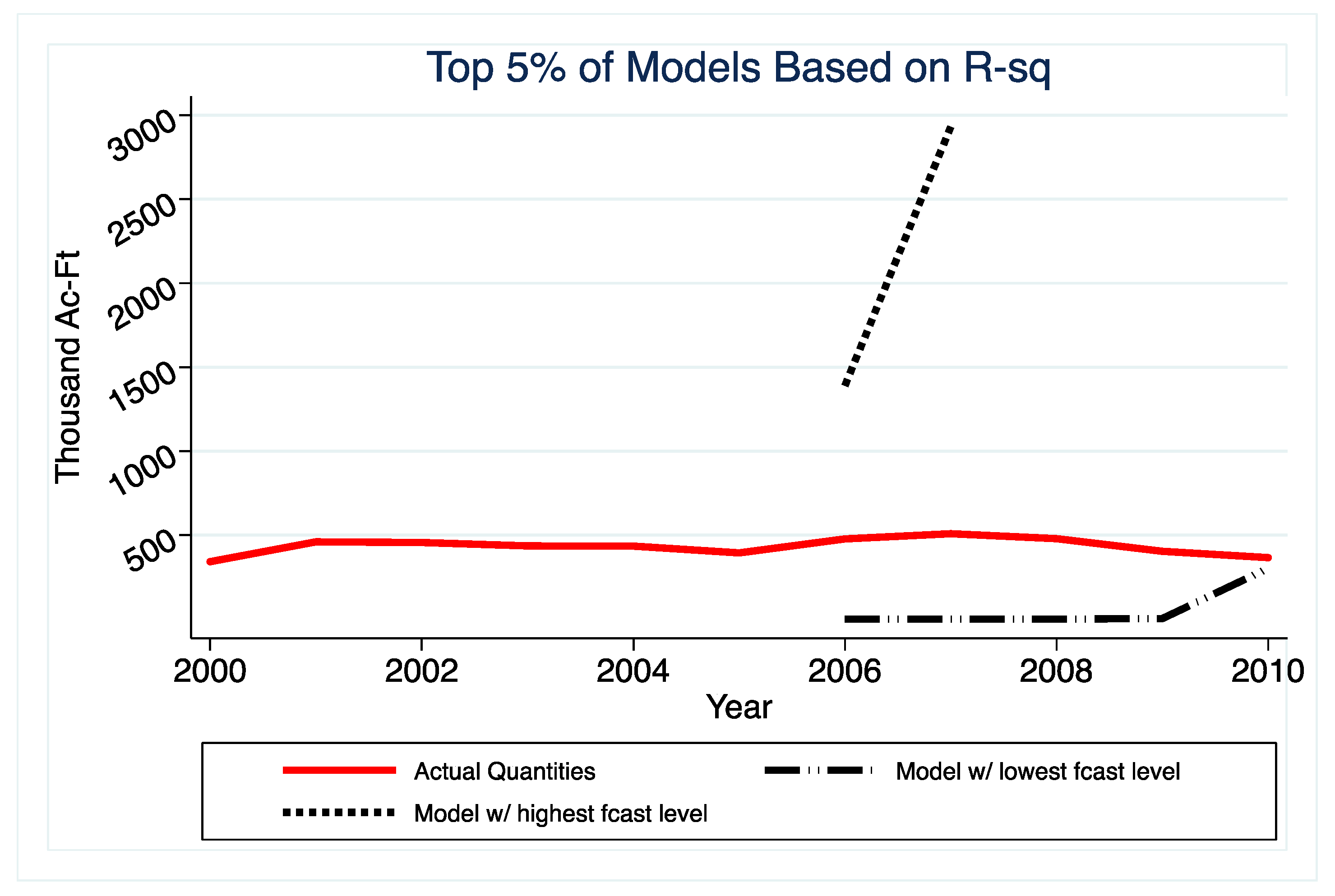
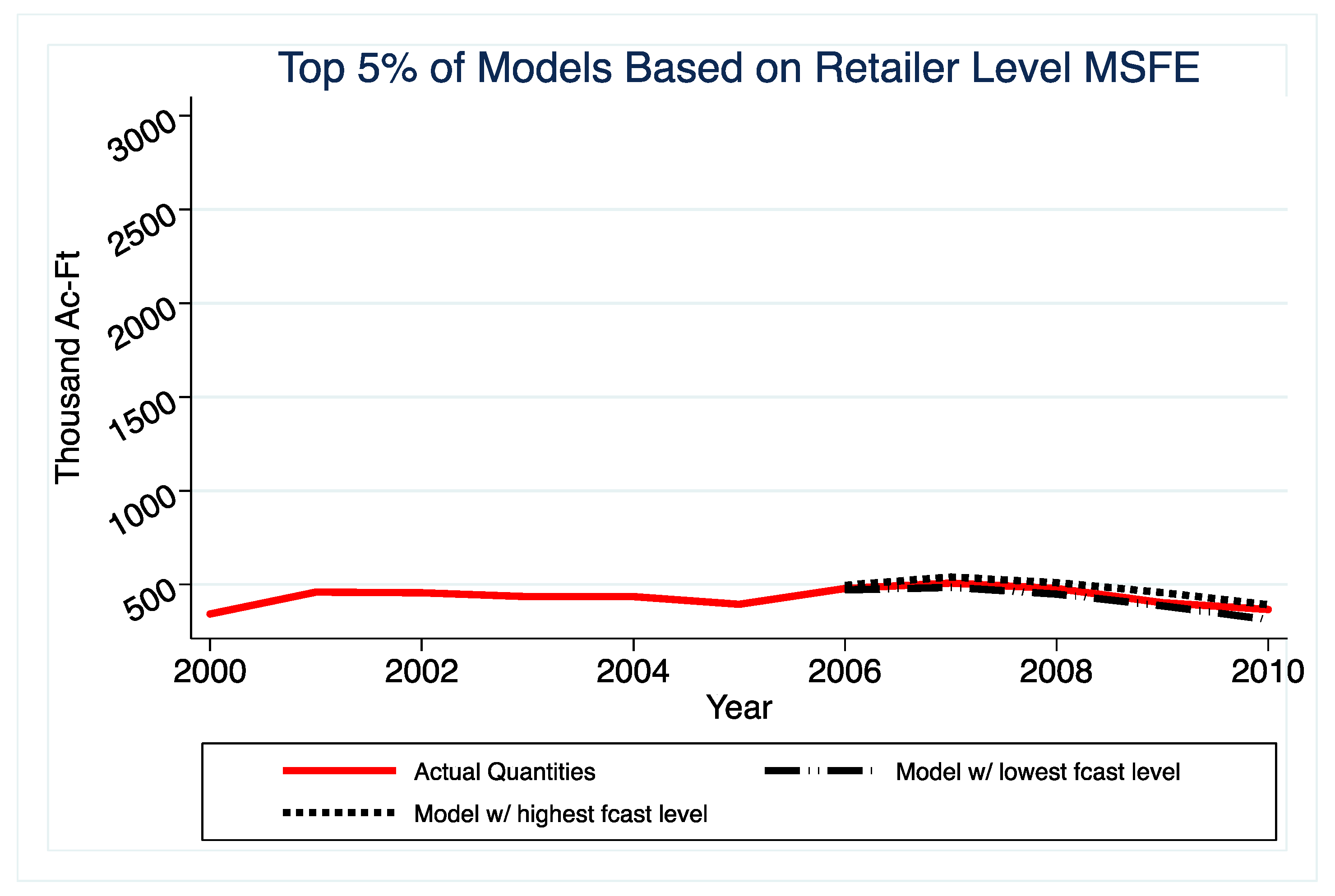
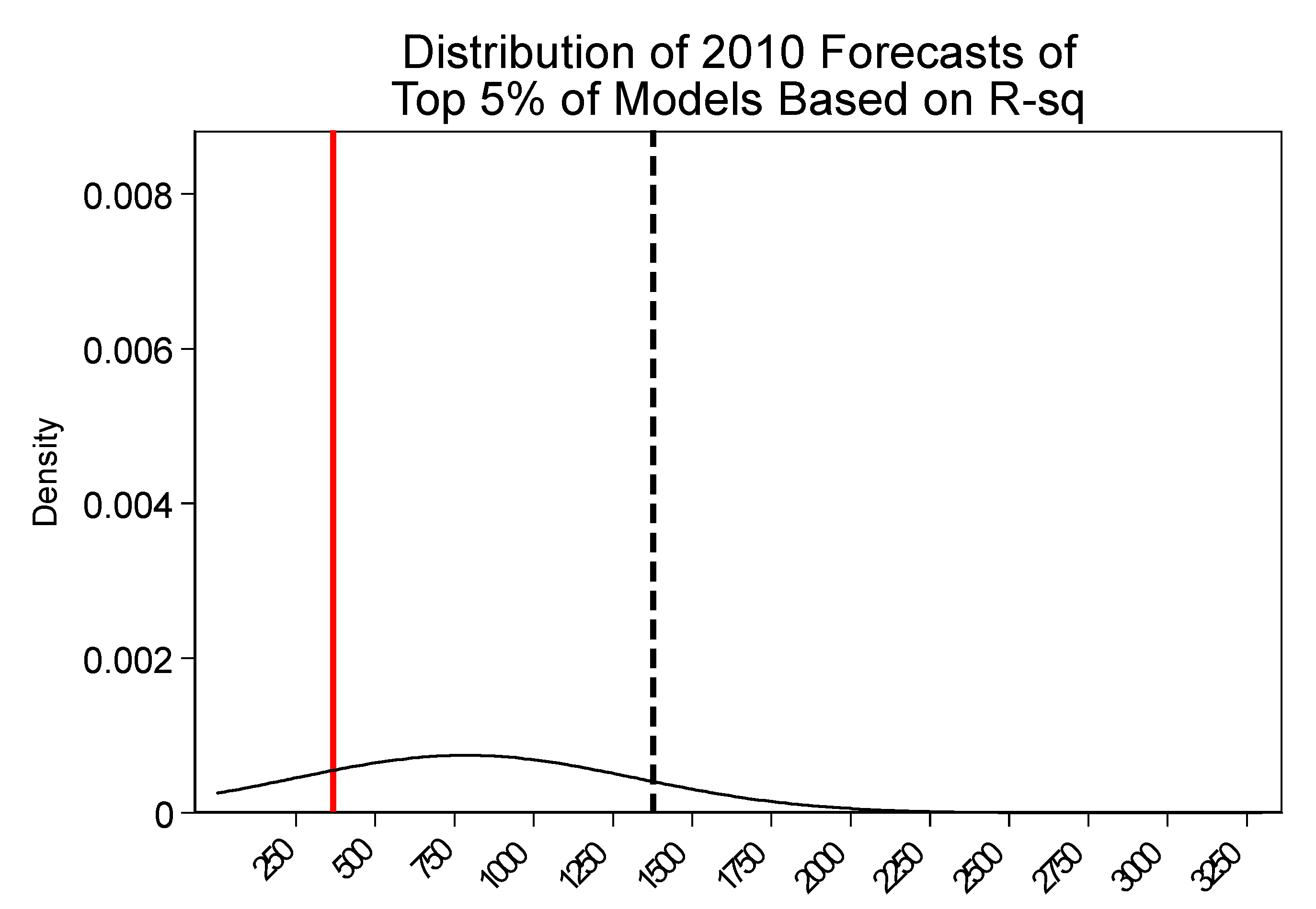
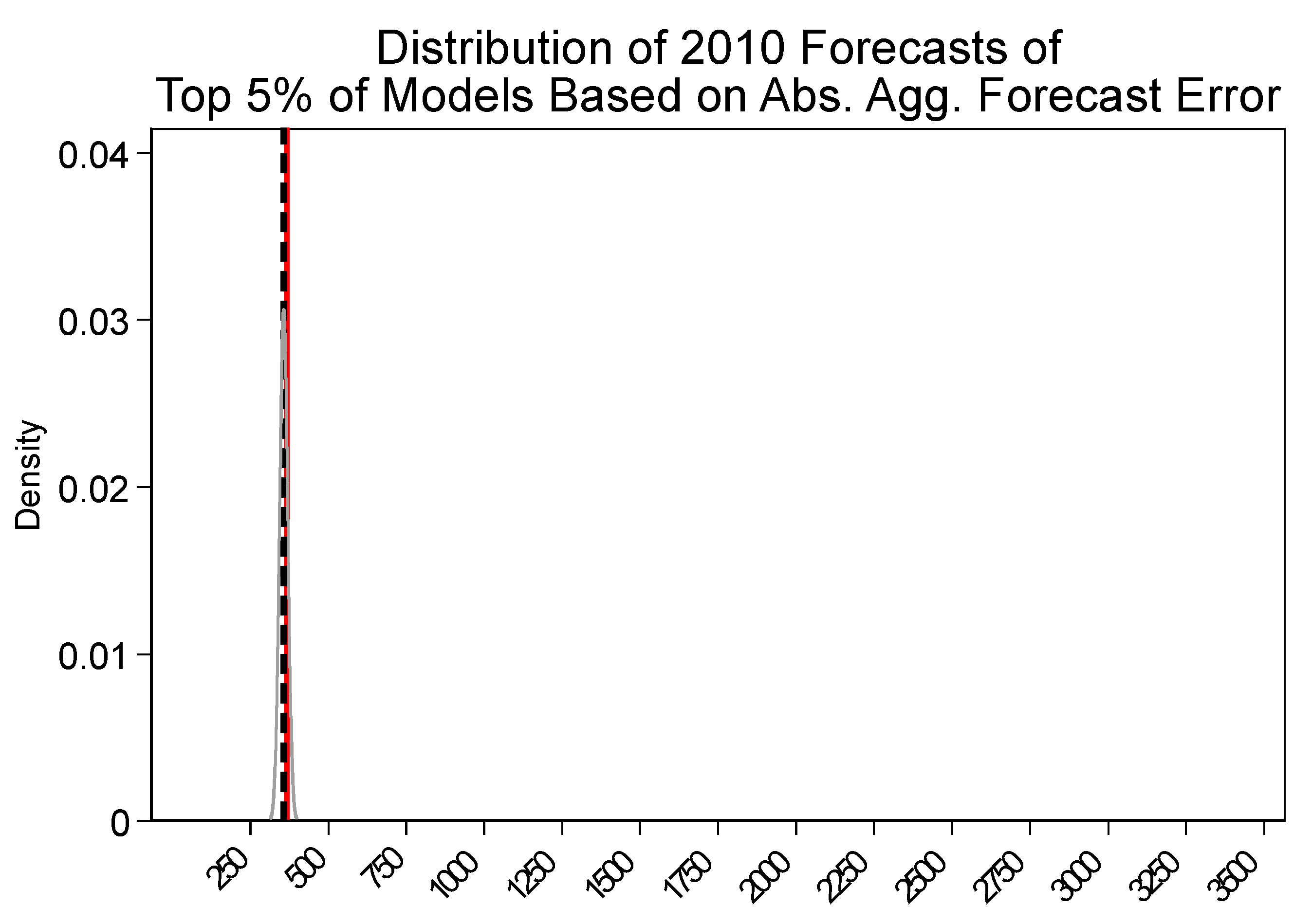
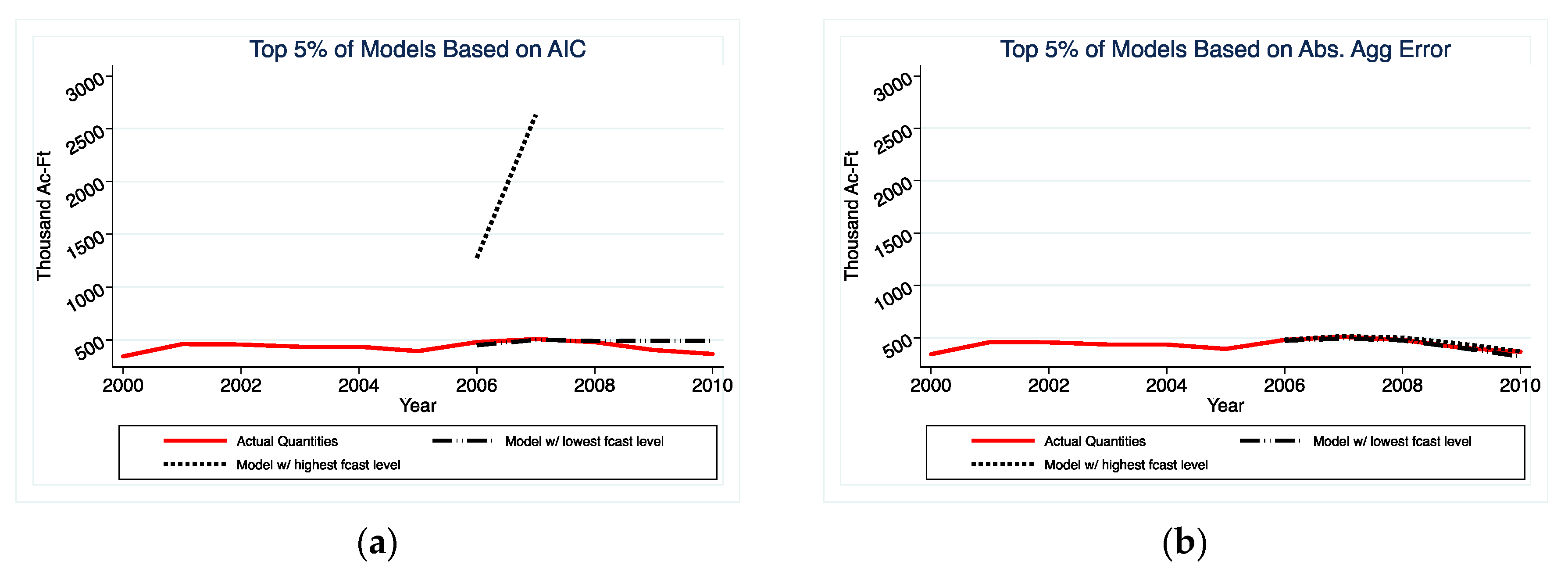
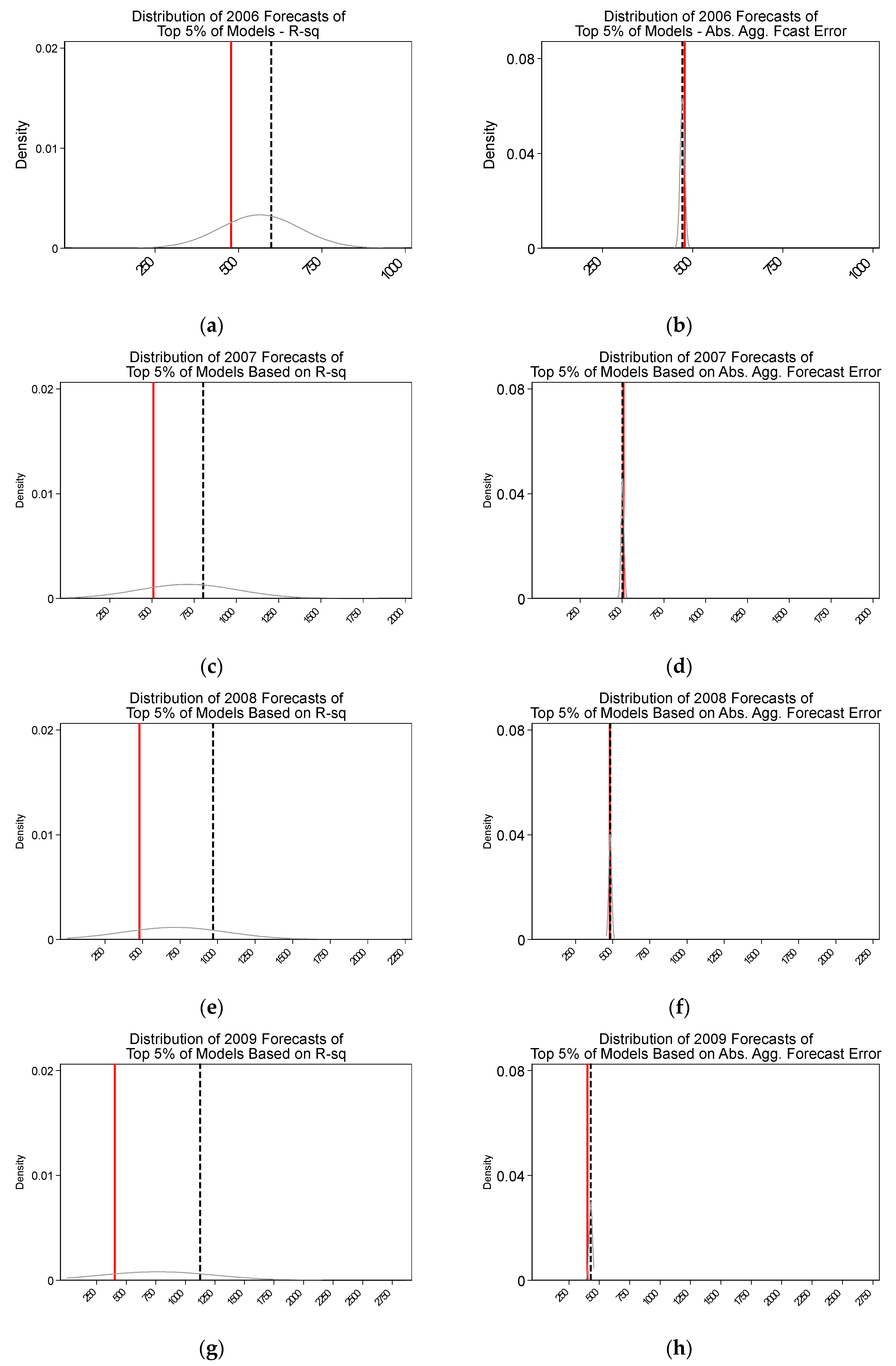
The results indicate that selecting models solely based on in-sample fit will yield poorly performing models when forecasting CII water use out-of-sample. Specifically, we demonstrate that the predictions that are generated by the highest R-squared models are highly dispersed around the actual value, relative to those that are generated by the models with the lowest absolute error. While it is known that models selected on in-sample fit can perform poorly out-of-sample, this paper brings the magnitude of the problem in the CII water forecast context to the attention of water planners. Equally important, the analysis contrasts variation in forecasts generated by prediction models that were selected based on different criteria. This highlights that decision-makers should consider a range of forecasts generated by a suite of the “best”-performing models.
These findings suggest that water planners, the forecasts of whom are often used to guide water policy, can avoid large errors by taking out-of-sample prediction performance into account when selecting models to forecast CII water use, which is a relatively small adjustment to their procedures.
The path followed in this paper is similar to the one used in Auffhammer and Steinhauser [
60] for forecasting CO
2 emissions. They use 41 years of state-level data to test about 27,000 models and compare the out-of-sample forecasting performances of benchmark models from the related literature and the ones that they find to be best under the aggregate error criterion. They find that benchmark models, which are calibrated against in-sample performance criterion, are likely to overestimate CO
2 emissions, which might be consequential in climate policy and international agreements.
In a similar spirit, this study compares the out-of-sample performances of the models that would be selected under various in- and out-of-sample criteria given the available dataset. Our findings highlight that the model selection criteria determine CII water use forecast performance.
The rest of the paper proceeds as follows: the geographical scope of the study, summary of the data, econometric model, and the details of performance criteria are provided in
Section 2.
Section 3 presents and discusses the results, and
Section 4 concludes.


