LSTM-Based Deep Learning Model for Predicting Individual Mobility Traces of Short-Term Foreign Tourists

Abstract

The increasing availability of trajectory recordings has led to the mining of a massive amount of historical track data, allowing for a better understanding of travel behaviors by revealing meaningful motion patterns. In the context of human mobility analysis, the problem of motion prediction assumes a central role and is beneficial for a wide range of applications, including for touristic purposes, such as personalized services or targeted recommendations, and sustainability studies related to crowd management and resource redistribution. This paper tackles a particular case of the trajectory prediction problem, focusing on large-scale mobility traces of short-term foreign tourists. These sparse trajectories, short and non-repetitive, lack spatial and temporal regularity, making prediction analysis based on individual historical motion data unreliable. To face this issue, we hereby propose a deep learning-based approach, taking into account the collective mobility of tourists over the territory. The underlying semantics of motion patterns are captured by means of a long short-term memory (LSTM) neural network model trained on pre-processed location sequences, aiming to predict the next visited place in the trajectory. We tested the methodology on a real-world big dataset, demonstrating its higher feasibility with respect to traditional approaches.

1. Introduction

Human mobility analysis has gained increasing popularity due to the recent growth in people’s location information availability in the form of massive trajectory data sets. Motion behaviors can be passively collected by mobile phones in terms of cell tower connection or GPS signal, or even actively shared by users on social media platforms. These large volumes of geo-located data enable the opportunity to reveal and integrate motion patterns in a wide variety of contexts [1,2], from recommendation systems [3,4] to mobility modeling applications for smart city and smart enterprise [5,6].

The rise of positioning technology and motion data availability has particularly boosted location prediction analysis, which has become a very active research area in the big picture of location-based services. Location prediction is interpreted as inferring the short-term future location of an individual, leveraging his/her current place, past motion activity, and possibly additional side information. Depending on the context, it may imply very different problems and approaches, comprising motion flow modeling [7,8,9], individual large-scale mobility analysis [10,11,12], and very fine resolution systems [13,14,15].

While the majority of works dealing with the prediction of individual mobility traces are set in contexts with a high level of spatial and temporal regularity (e.g., motion activity of users in everyday life), our paper contributes to extend trajectory prediction analysis in the opposite direction, when individual motion regularity is lacking due to the non-repetitiveness of single mobility traces.

Our focus and intended application is related to tourists’ mobility within the growing field of smart tourism. Smart tourism integrates tourism resources with information technologies to design intelligent services to provide valuable outcomes to tourists and tourism-related industries. The development of smart tourism is particularly embodied in four main aspects, namely tourism experience, tourism management, tourism service, and tourism marketing [16,17,18,19]. The tracking and recording activity of space-time paths of individual tourists is inserted in this big wave of tourism mining, not as an ultimate purpose, but as a mean of providing valuable knowledge of tourists’ mobility and travel behaviors. However, although spatial-temporal trajectory data have been widely utilized in studies of tourists’ behavior, their use has been mainly limited to descriptive purposes at the level of clustering and pattern analysis [20,21,22,23]. But if forestalling actions require consideration, predictive investigations become an essential tool.

Our case study targets short-term tourists in a foreign country. Foreign tourism is major source of income for the tourism industry and it is an area of investigation for public and private organizations. Most destination strategies define measures specifically designed for foreign tourists, which have different behaviors and spending patterns compared to domestic users. For this reason, the unfolding of their tourism experience is used to understand and possibly leverage the insights to improve tourism policies and decision-making.

While in everyday life a person’s mobility is described by a significant probability of returning to a limited number of highly frequented locations (e.g., home and workplace) [24,25,26], the natural characterization of foreign tourists’ motion behavior is based on short and non-repetitive trajectories of users moving in areas they have never been to. The lack of individual historical location data leads methods relying on a set of individual pre-recorded motion trajectories to performing poorly when applied to traces covering areas that are unfamiliar to the user; a prediction algorithm solely based on a sequential approximation of a single probability distribution is not effective in this case. In addition, the focus on large-scale mobility often implies a very wide territory, introducing further problems such as trajectory data sparseness and a multitude of locations, involving the curse of dimensionality.

The proposed method aims to overcome these issues with the use of a deep learning-based approach that leverages the collective mobility of users over the territory. The method consists of a long short-term memory (LSTM) neural network trained on pre-processed location sequences to learn the underlying patterns of tourists’ motion activity. Original traces are first transformed into discrete location sequences, and are subsequently fed into a deep neural network model composed of embedding and LSTM layers. The model captures motion patterns directly from mobility traces, without requiring any manual feature extraction. Each individual user’s mobility prediction is therefore based on the collective analysis of tourists’ behavior over the territory. For a wider application in various contexts, we do not resort to any additional information besides the users’ motion traces, since useful secondary information is not available in many cases. In this way, the model can be applied to a variety of geo-located data types, as long as the recorded positional data generated by users can be properly organized into mobility traces in the form of sequences of locations.

Experiments on a real-world large-scale big dataset prove the higher feasibility of our forecasting method with respect to traditional approaches in this mobility regime, standing out as a potentially beneficial methodology for many real-life applications, including touristic services for personalized recommendations, targeted advertisement, and sustainability studies related to crowd management and resource redistribution. In general, this study contributes to the expansion of tourists’ mobility analysis in the direction of actively integrating artificial intelligence into the tourism sector.

2. Related Work

The rise of motion data availability has boosted the interest in human mobility analysis, establishing various methods for trajectory data mining [27,28] to either describe the observable motion behavior [29] or to predict future activities [30].

Location prediction has a central role in human mobility analysis and is applied to numerous tasks such as crowd management, congestion prediction, transportation planning, and place recommender systems [31,32]. In the past few years, plenty of predictive models have been suggested, leveraging various methods including Markov models [33,34] and data mining approaches [35,36,37]. Previous research on location prediction can be roughly split into two broad groups: motion regularity-based methods and multiple mobility-based methods.

The first group is based on the regularity of individual user’s motion history. Since most people tend to follow regular motion patterns in daily life, often returning to the same few locations, their personal past mobility is a valuable factor to predict their future trajectories [24,25,26]. Therefore, the majority of works on predicting a person’s next visited location rely on historical motion data collected from this person exclusively, evaluating the regularity patterns in human mobility by learning individual, frequent traveling routes [38,39]. In this sense, the most common approach is the use of Markov models, representing locations as states and movement between locations as transitions [11,12,40]. States are defined by partitioning space into grids or reference points, and transition probabilities are defined by counting each user’s transitions, identifying the most likely next destinations for each current location. This type of model achieves good performances in the presence of long, pre-recorded motion trajectories of the particular user under study.

The second group comprises methodologies combining individual past locations with collective motion information from multiple users. A subgroup is represented by collaborative filtering to find similarities among users’ preferences in frequently visited destinations [41]. This includes methods for classifying users’ preferences into point of interest categories [42] and recommendation systems based on generic, top interesting places or personalized location matching [43]. Another subgroup focuses on geographical elements, predicting the next locations based on the definition of features for each place and the relationships between places. These methodologies do not model individual preferences or similar preferences among users, but make predictions by using geographical statistics [44,45]. A final subgroup includes motion pattern mining techniques and prediction algorithms combining individual current movements with historical collective data to find frequent patterns and co-occurrences of locations. The methods comprise ensemble probabilistic algorithms [46,47], feature-based machine learning methodologies [48,49], and deep learning models [50,51] to predict users’ locations over time, based on individual and collective behaviors.

In general, when people rarely share their history of past visited places with other users, location prediction methods based on previously seen locations of an individual user are likely to be chosen over other methodologies. However, in the case of irregular individual motion patterns, short data history users, and non-repetitive mobility behaviors, prediction algorithms approximating single probability distributions are not reliable and multiple mobility-based methods may be preferred. Moreover, it is worth mentioning that a large number of methods enrich trajectories with further context data, such as prior knowledge of motion information (e.g., acceleration, orientation) [11], external data (e.g., weather, social media analysis) [52,53], or user-specific features (e.g., home and workplace, user specific preferences) [44,54,55,56,57]. In these cases, the main disadvantage is of a practical nature, since secondary information is often insufficient or not available.

Over the last decades, academics and practitioners have increasingly approached the study of tourists’ movements [20,58,59] and how to guide practical measures based on these findings [60,61,62]. Most studies focused on mapping and modeling movements between locations [21,63], as tourist destinations are involved in a complementary relationship [64,65]. These include travel itinerary models [66] and spatial pattern examination of travel flows [67,68], often leveraging a variety of measures within the study framework [21,69]. Only few studies, however, exclusively involved international visitors [70,71]. While the interest in mining movement patterns of tourists has been prominent, and studies are developing fast for collectively estimating the overall amount of visitors within single destinations [72], the explicit prediction of individual short-term tourists’ mobility traces still requires further expansion, being mainly based on Markov approaches for modeling location transitions [47,58,59].

This paper therefore introduces a deep learning model to predict individual trajectories of short-term foreign tourists. Its characteristics comprise: leveraging the collective mobility of people to predict individual traces, falling in the category of multiple mobility-based algorithms; learning mobility patterns without any manual feature extraction or secondary context data by simply feeding the model with sequences of locations, from a purely data-driven perspective; explicitly designed to predict the next location of a user, specifically when a very short data history is known about that user. The use of LSTM is tested in this particular mobility regime of short and non-repetitive traces to assess its feasibility when applied to large-scale movements of visitors in a foreign country.

3. Methodology

The proposed prediction method aims to model patterns hidden in the historical motion data of multiple people, in order to identify the most likely future movement of an individual user. Given a short mobility trace sampled at a given time step, the solution of our model consists of inferring the future visited location in the next time step. This section reports the details of the proposed methodology, from trajectory pre-processing to deep learning modeling.

3.1. Trajectory Pre-Processing

The first step of the path from original mobility traces to location prediction is characterized by trajectory discretization, a pre-processing phase transforming raw traces into the input for the neural network model.

An original mobility trace is described by a series of chronologically ordered track points $T=\left\{p_i\right|i=1,2,3,\dots ,N\}$, generated by an individual user, whereby each point is defined by a coordinate pair enriched with a time stamp $p_i=\left({lon}_i,{lat}_i,t_i\right)$. The trajectory discretization task consists of aggregating continuous values of longitude and latitude into discrete locations and transforming the continuity of time into fixed time steps. This results in a pre-processed trajectory in the form of a sequence of locations $\left({LOC}_1,{LOC}_2,\dots ,{LOC}_N\right)$, where, given a time step unit $t$, locations refer to time $\left(t,2t,\dots ,Nt\right)$. Time information is therefore encoded in the position along the sequence and the location associated to each time step is chosen as the one identified by the majority of track points recorded within that time period. The length of the time step is case specific, depending on the data source and the prediction problem: a short unit increases fragmentation in the presence of discontinuous traces and low time resolution data, a long unit may compromise a proper trajectory representation affecting prediction results. Moreover, even spatial resolution varies according to the data source, and may be further discretized (e.g., through clustering, reference point definition, and grid-based approaches) in relation to the time resolution and the specific purpose of different applications (e.g., prediction of motion traces over a whole country or mining city-level mobility). This is particularly suggested when trajectories are very sparse and there are many locations with only very few occurrences. In addition, because human mobility is not generally uniformly distributed over the territory, locations that are potentially inaccessible or irrelevant should be discarded; only those locations that are seen by a sufficient amount of people should be considered, avoiding bias samples in the data and worthless computational effort. The result should consist of a set of fixed points (or areas) over the territory, each of them associated with a particular unique identifier. A pre-processed trajectory is made of a sequence of these discrete locations unfolding in fixed time steps.

3.2. Deep Learning Model for Trajectory Prediction

The collection of the pre-processed trajectories from multiple users, in the form of sequences of unique location identifiers, is used as input data to the deep neural network model. The model is made of three building blocks: an embedding layer, a block of one or more LSTM layers, and a softmax layer. Each location identifier is initially associated to a particular corresponding embedding vector, encoding input trajectories into sequences of embeddings that are subsequently fed to the LSTM block, made of stacked LSTM neural network layers. The final trajectory representation, output vector of the last LSTM layer, becomes the input of a softmax layer for generating the probability distribution of the next predicted location in the trace. A graphic exemplifying overview of the whole model, with a block of two LSTM layers, is illustrated in Figure 1.

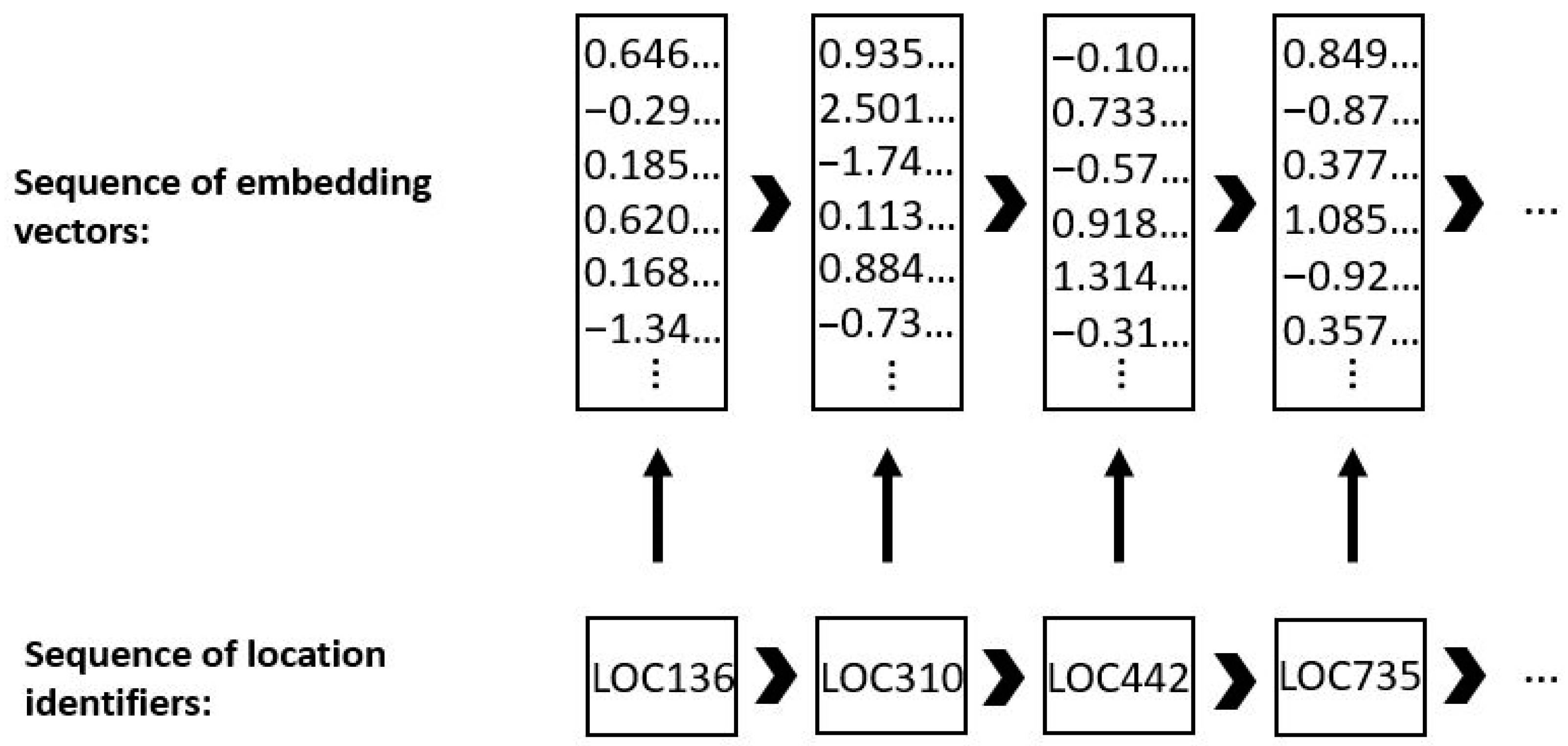
3.2.1. Embedding Layer

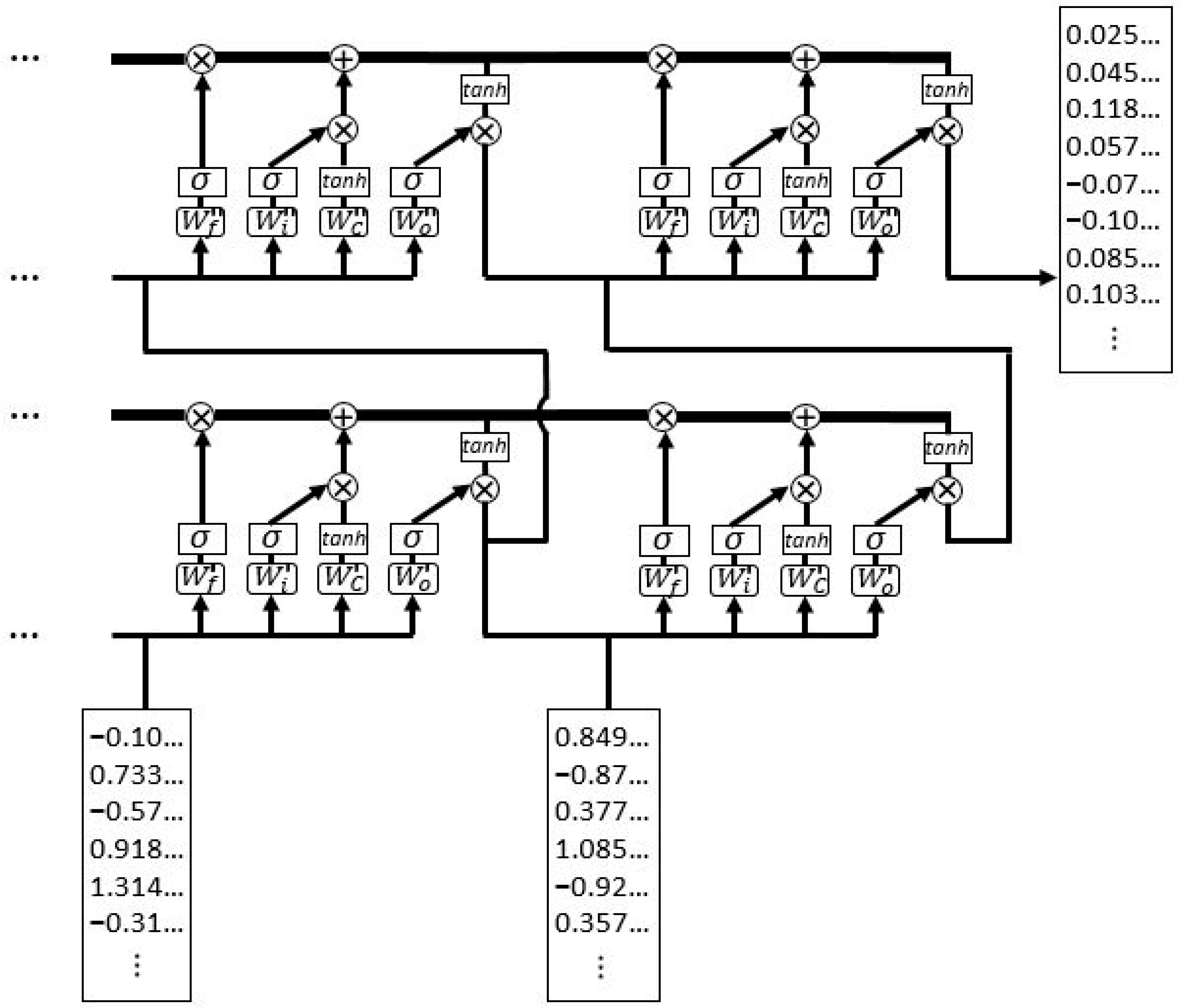
To limit the problems of the curse of dimensionality, trajectory sparseness, and computational inefficiency, we replace traditional representations such as one-hot by associating each discrete location with a low-dimensional dense vector (embedding). This is done by means of an embedding layer, transforming sequences of discrete location identifiers into sequences of dense vectors before they are fed to the LSTM block, as depicted in Figure 2. In particular, each location is initially defined by a random vector of a pre-defined size, whose values are updated during the training process; just like other model parameters, embeddings are tweaked, through backpropagation, on the basis of the prediction outcomes. Over training, they assume a meaningful mathematical representation as vectors of continuous values, whereby locations that are often co-occurring in the same traces share similar representations in this embedding space.

3.2.2. LSTM Block

The next stage consists of the LSTM block. LSTM [73] is a complex recurrent neural network type, whose repeating module is composed of four different neural networks interacting between each other. The network processes an input sequence one element at a time, receiving, at each step, two sources of input data: the current vector of the data sequence concatenated with the output vector of the network module at the previous step. The information flows through the network modules, encoded in the cell state, and is modified by the four neural network structures until the end of the sequence is reached. The output at the last step is the final vector characterization of the sequence, which is subsequently used for the actual prediction task. If the LSTM block contains multiple LSTM layers, the final trajectory vector is represented as the output, at the last step, of the last layer. In general, the first LSTM layer is fed with the input sequence, the second layer is fed with the output of the first layer, and so on. Figure 3 displays a visual representation of the LSTM block; the example shows the last two steps of an embedding sequence and a block of two LSTM layers.

Equations (1)–(6) report the formulas describing the functioning of a repeating module of LSTM, given an input vector $x_t$; the forget gate (1) defines the information to be deleted from the cell state; the input gate (2) decides which values to update; the tanh network (3) determines a vector of new values to be added to the state; the new cell state (4) is obtained by filtering the old cell state through the forget gate, and by adding the combination outcome between the input gate and the tanh network; the output gate (5) defines which parts of the cell state to output; and the final LSTM output (6) results from the multiplication between the output gate and the tanh of the new cell state.

$$f_t=\sigma \left(W_f·\left[h_{t-1},x_t\right]+b_f\right)$$

(1)

$$i_t=\sigma \left(W_i·\left[h_{t-1},x_t\right]+b_i\right)$$

(2)

$${\tilde{C}}_t=\tan \mathrm{h}\left(W_C·\left[h_{t-1},x_t\right]+b_C\right)$$

(3)

$$C_t=f_t\ast C_{t-1}+i_t\ast {\tilde{C}}_t$$

(4)

$$o_t=\sigma \left(W_o·\left[h_{t-1},x_t\right]+b_o\right)$$

(5)

$$h_t=o_t\ast \tan \mathrm{h}(C_t)$$

(6)

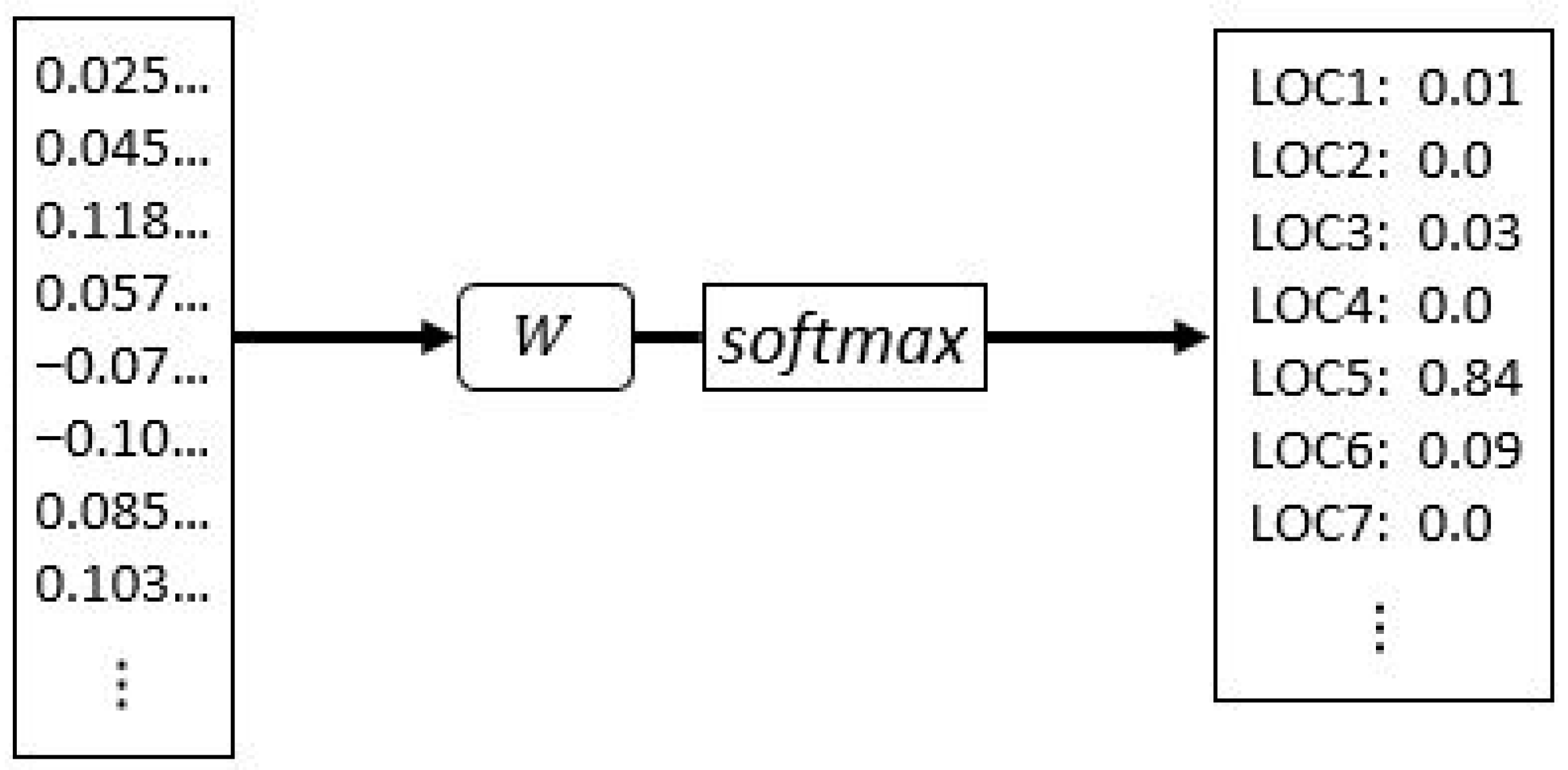
3.2.3. Softmax Layer

The predicted next location is explicitly disclosed by means of a softmax layer on top of the LSTM block. The softmax layer is a simple, fully-connected neural network followed by a softmax activation function. It receives the final trajectory vector characterization as an input, and outputs the predicted probability distribution for the next potential location, as shown in Figure 4.

Equation (7) reports the description of the softmax layer, where $h_{last}$ represents the output of the last LSTM layer at the last step and $n\_LOC$ is the total number of locations.

$$(LOC=j|h_{last})=\frac{\exp \left(W_j{h}_{last}^{\prime }+b_j\right)}{{{\displaystyle \sum }}_{k=1}^{n\_LOC}\exp (W_k{h}_{last}^{\prime }+b_k)}$$

(7)

3.2.4. Model Training

Prior to being fed into the neural network model, location sequences are scanned by a sliding window, determining the training features and the target variable. The window moves forward by one location until the end of each sequence, defining multiple segments of fixed length as input sequences to the deep learning model. The segment length represents the amount of past motion activity taken into account for learning to predict the future location (e.g., predicting the next location based on the last six hours of a user’s mobility). Its choice, besides strongly depending on the applications and dataset restrictions, is closely related to the time resolution of the sequence, whereby a higher time resolution determines a larger number of locations describing the past motion activity.

The deep learning model is fed with a collection of these segments, where, for example, a window length equal to four locations would define a sequence (${LOC}_{t-3}$, ${LOC}_{t-2}$, ${LOC}_{t-1}$, ${LOC}_t$) as input features to the model and the location ${LOC}_{t+1}$ as the target variable. The model training maximizes the log probability, with respect to the weights of every layer (embedding, LSTM, and softmax), of observing the correct next location, given the sequence of past locations. The process relies on backpropagation and mini-batch stochastic training to determine in which direction the weights are adjusted.

The prediction of a location sequence is therefore based on the collective historical mobility of people, identifying the most likely next location as the one having the highest probability according to the output of the model.

4. Experiment

The current section introduces the dataset used for the prediction task and reports the description and results of the experiments conducted. A particular focus is given to the evaluation of results, which are compared to traditional approaches and are analyzed according to different motion characteristics. The proposed model was implemented and executed on TensorFlow (Google Brain, Mountain View, CA, USA), using AWS EC2 p3.2xlarge GPU instance.

4.1. Dataset

To properly describe the general large-scale motion activity of foreign tourists, we used a real-world dataset comprising seven months of anonymized mobile phone call detailed records (CDRs) of roamers in Italy. In order to present meaningful findings, it is indeed important, especially when dealing with wide territories, to make use of a sufficiently large and complete dataset, whose trajectories redundantly cover the study area. CDRs have been widely used in human mobility studies [74,75,76,77], reporting the detected mobile phone activities enriched with the time stamp and the position of the device in terms of the coverage area of the principal antenna. We only took into account short-term visitors, recorded to be located in the country for a maximum of two weeks. In addition, we discarded those users that appeared to be completely stationary. Foreign visitors’ mobility was therefore represented by short traces and non-repetitive behaviors.

The erratic profile of mobile activity, represented by sparse connection events, may critically fragment mobility traces, making it difficult to create continuous location sequences. To limit the fragmentation problem and define proper trajectories, we pre-processed traces into sequences unfolded in 1 h time step; the prediction problem is formulated as predicting the location of a user in the next hour. In particular, if more than one track point was recorded in the same hour, the location associated to the majority of those recordings was chosen to identify the current position of the user. Given the wide territory, the choice of the time step unit, and our focus on large-scale movements, a minimum spatial resolution of 2 km was selected. Reference points were defined as the antennas subjected to the highest number of connections within the minimum spatial resolution, projecting the other ones to the closest reference point. Furthermore, we discarded very rare locations, identified by just a few tens of recorded events. Being mostly randomly visited, they are not significantly involved in the overall travel behavior of foreign visitors in Italy. Nevertheless, specific characteristics of different datasets may provide an influence on parameters such as time and space resolution, and a choice of different values can be suitable for different applications.

The final dataset consists of 1 h encoded sequences of 5903 possible unique locations over the Italian territory. To appropriately focus on short motion behaviors and to make complete and proper utilization of the dataset, represented by relatively short continuous traces, we set a window length equal to 6 h (6 locations), determining a total of 13 million trajectory segments (with a median displacement per segment of 36.1 km) generated by 1.4 million users. We believe this large amount of data is representative of the overall real motion behavior of foreign tourists.

4.2. Experimental Settings

We designed the neural network model using an embedding size of 100 dimensions and a block of two LSTM layers having a hidden size of 4000 neurons each. The training process was based on cross-entropy cost function, mini-batches, and Adam optimizer [78]. To evaluate the performance of the model on previously unseen data, we randomly split the dataset into a training set and a test set, containing 80% and 20% of the users, respectively.

For a better evaluation of the results, we compared the achieved prediction accuracy with traditional approaches involving the use of Markov modeling, which is widely applied in location prediction problems. Locations are represented as states and movements between locations as state transitions. The creation of a transition matrix identifies the most likely next destinations for each current location [33]. We reported three different Markov model types as comparison baselines for our methodology:

-

Personal Markov model. Transition probabilities were calculated by counting each single user’s transitions, modeling individual movement patterns.

-

Global Markov model. First-order probability distributions were calculated by counting the collective state transitions of all users, modeling collective movement patterns.

-

Variable-order global Markov model. The principle of the longest match was applied to select which global Markov model order to adopt to calculate the transition probabilities; for a given location sequence, the collective prediction probability distribution was computed on the set of training sequences matching its longest suffix.

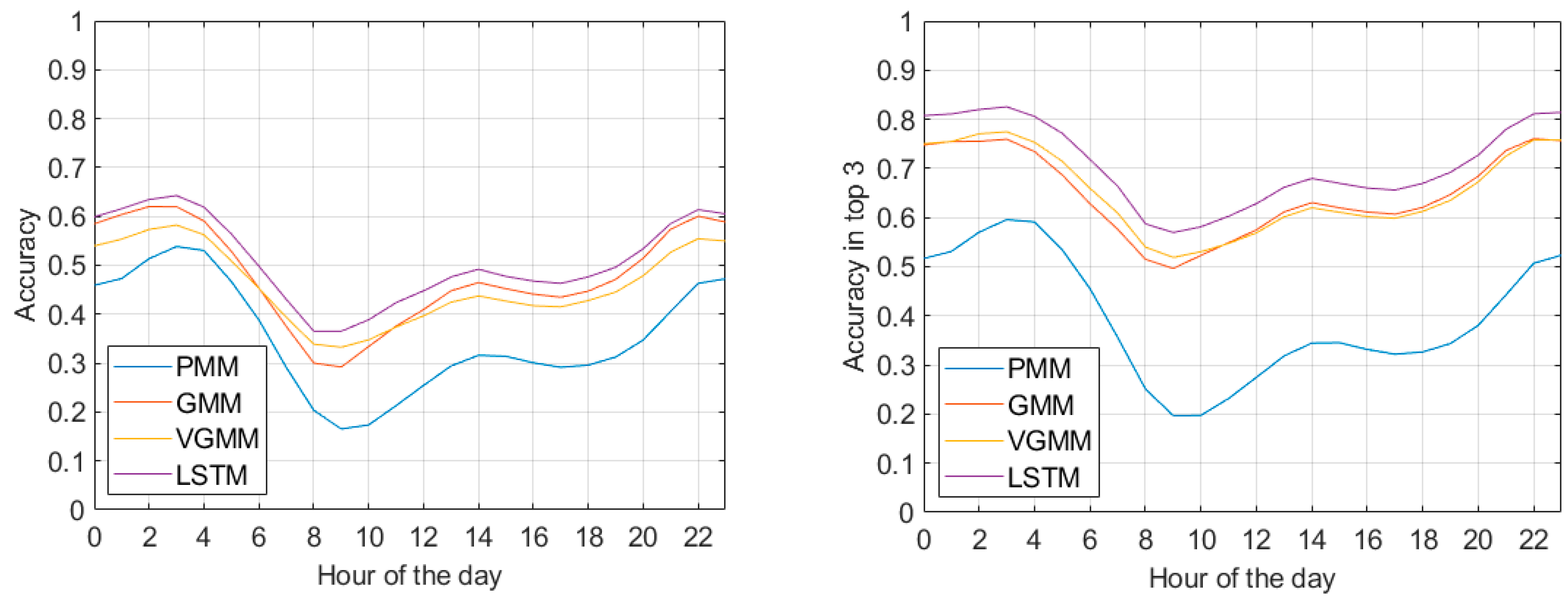
4.3. Results

Table 1. Overall performance comparison between our methodology (LSTM) and the Markov baseline approaches, namely personal Markov model (PMM), global Markov model (GMM), and variable-order global Markov model (VGMM).

	Accuracy	Accuracy in Top 3
PMM	0.3373	0.3717
GMM	0.4822	0.6508
VGMM	0.4553	0.6445
LSTM	0.5076	0.7013

reports the comparison results in terms of accuracy and accuracy in top 3 (if the correct label corresponds to one of the top three predicted locations, the accuracy is 1, otherwise it is 0; the result is the average for each testing trajectory). Our model (LSTM) outperformed the Markov approaches, yielding a 5% improvement compared to the best baseline, the global Markov model (GMM), 10% improvement compared to the variable-order Markov model (VGMM), and 33% to the personal Markov model (PMM). The accuracy in top 3 confirmed this trend, showing a 7% improvement of our model with respect to GMM, 8% to VGMM, and 47% to PMM.

Reasonably, PMM, which was solely based on individual mobility and ignored the collective motion behavior, had the lowest scores in this regime of short and non-repetitive traces. GMM and VGMM, which considered the collective mobility of all users, greatly improved performances, with the first-order model surpassing the variable-order model. LSTM determined a further increment, exceeding the best baseline of 2.5 percentage points in terms of accuracy and 5 percentage points in terms of accuracy in top 3.

Moreover, we analyzed how different trajectory characteristics affect prediction. The idea was to evaluate the influence of different values of motion features, such as the traveled distance and radius of gyration, on the prediction performances.

Table 2. Accuracy (and accuracy in top 3 in brackets) comparison for different values of traveled distance.

Trav. Dist. =	≤10 km	10–25 km	25–50 km	50–100 km	≥100 km
PMM	0.4645 (0.5088)	0.4240 (0.4901)	0.3260 (0.3639)	0.2613 (0.2796)	0.1665 (0.1689)
GMM	0.5495 (0.7805)	0.5648 (0.7412)	0.4988 (0.6534)	0.4494 (0.5845)	0.3391 (0.4582)
VGMM	0.5788 (0.7945)	0.5033 (0.7201)	0.4312 (0.6270)	0.3979 (0.5656)	0.3212 (0.4630)
LSTM	0.5938 (0.8172)	0.5696 (0.7933)	0.5061 (0.7036)	0.4633 (0.6293)	0.3803 (0.5270)

shows the accuracy and accuracy in top 3 (in brackets) for different values of traveled distance within six hours prior to prediction. Five bins were selected: ≤10 km, 10–25 km, 25–50 km, 50–100 km, and ≥100 km. Comparing accuracy, despite an overall tendency of decreasing performance when the traveled distance increases, PMM always performed very poorly, while GMM and VGMM achieved remarkable results for mid and short distances, respectively. In particular, GMM substantially outperformed VGMM for mid-range values (10–100 km), but was overcome by the latter for very short distances (≤10 km). LSTM always exceeded every baseline, even if it only slightly outperformed GMM for mid-short distance values (10–50 km). It is worth noticing how LSTM largely overcame the other methods for very long distances (≥100 km). Moreover, its accuracy in top 3 was consistently much higher than every baseline for each distance bin.

Table 3. Accuracy (and accuracy in top 3 in brackets) comparison for different values of radius of gyration.

ROG =	≤3 km	3–10 km	10–32 km	≥32 km
PMM	0.4539 (0.5213)	0.3650 (0.4078)	0.2974 (0.3089)	0.1880 (0.1899)
GMM	0.5496 (0.7859)	0.5246 (0.6880)	0.4719 (0.6038)	0.3548 (0.4729)
VGMM	0.5661 (0.7923)	0.4578 (0.6668)	0.4218 (0.5846)	0.3371 (0.4781)
LSTM	0.5891 (0.8229)	0.5299 (0.7480)	0.4849 (0.6426)	0.3955 (0.5404)

reports the accuracies for different values of radius of gyration (ROG), in bins of ≤3 km, 3–10 km, 10–32 km, and ≥32 km. These results reinforce the observations reported in the previous case, such as the general tendency of decreasing performance as the ROG value increases, the overall poor achievements of PMM, the good results of VGMM for very small values (≤3 km), and the remarkable performance of GMM for mid-range values (3–32 km). Again, LSTM always outperformed the baselines, only slightly beating the GMM accuracy for the 3–10 km bin, but greatly overcoming the other methods for very large ROG values (≥32 km). As in the traveled distance case, its accuracy in top 3 was consistently much higher than the baselines for each of the ROG bins.

In addition, we observed the prediction variability at different hours of the day. Figure 5 displays the accuracy and accuracy in top 3 of the four methods over time, starting from midnight. Rush hours in the afternoon appeared to be more predictable than the ones in the morning, while accuracies significantly increased in the evening and night due to the higher regularity of mobility patterns during these hours. LSTM was shown to outperform the baselines for every hour of the day.

Performances were further explored based on the imbalance of the dataset, by evaluating results corresponding to popular and rare locations.

Table 4. Accuracy (and accuracy in top 3 in brackets) comparison for visited locations in different ranges of occurrence in the data. The percentage value in the first row refers to the amount of occurrences of each location in that column with respect to the whole dataset.

Amount of Data:	≥0.5%	0.1–0.5%	0.05–0.1%	≤0.05%
PMM	0.5169 (0.5485)	0.3809 (0.4147)	0.3280 (0.3600)	0.2624 (0.2986)
GMM	0.6872 (0.9305)	0.5398 (0.7659)	0.4745 (0.6511)	0.3925 (0.5095)
VGMM	0.7172 (0.9146)	0.5448 (0.7624)	0.4462 (0.6456)	0.3336 (0.5049)
LSTM	0.7372 (0.9459)	0.6024 (0.8210)	0.5039 (0.7151)	0.3925 (0.5660)

reports the accuracies for different ranges of location occurrences in the data, defining frequently visited locations and less visited ones. The columns from left to right identify specific groups of locations, where each location of each group represents, respectively, over 0.5% of the whole dataset, between 0.1% and 0.5%, between 0.05% and 0.1%, and less than 0.05%. As expected, there is a general drop of performance when passing from popular locations to rare ones. However, the superiority of LSTM is once again clearly exhibited.

Finally, we focused on the prediction errors to study the performance of our model in the particular case when it was not able to correctly identify the future visited location. We compared LSTM with GMM, the best baseline in terms of accuracy, to assess how their predicted locations differed when a misprediction occurred in both models. Figure 6 reports the bar graphs representing the error distance distribution of the segments that are wrongly predicted by both models. The error distance was calculated as the absolute distance between the wrongly predicted location and the real future location (to calculate the error distance of wrong predictions in top 3, we considered the predicted location, within the first three, having the shortest distance with the real location). The bar graphs highlight the overall tendency of LSTM to make mistakes with a shorter error distance than GMM.

We also studied the difference of error distance between the two prediction models, analyzing the corresponding mispredictions on the same segment. The bar graphs in Figure 7 display the subtraction $error\_distance\left(GMM\right)-error\_distance\left(LSTM\right)$ for wrong predictions and wrong predictions in top 3; a negative value indicates that the baseline provided a shorter error distance on a wrongly predicted segment; a positive value is in favor of our model. As depicted by the high bars on the right part of both graphs, there were a remarkable number of samples on which GMM tended to make prediction mistakes in the order of a few tens of km more than LSTM. Overall, our model, besides the higher prediction accuracy, also presented better results in terms of the shortest error distance.

4.4. Discussion

We proposed a method to predict individual mobility traces of short-term foreign tourists leveraging the collective large-scale motion behavior of people and a deep learning-based methodology adapted to process motion trajectories. The model relies on a recurrent neural network architecture composed of embedding and LSTM layers. We assessed the feasibility of such methodology on short, non-repetitive traces, revealing its potentiality for human mobility studies and applications.

In particular, our method was shown to outperform the widely used Markov model approaches based on location transition probabilities. The results reported how a probabilistic approach built on the motion behavior of a single individual performs very poorly in this mobility regime, proving the need for collective motion information. This collective mobility, however, consists of non-repetitive traces that clearly influence prediction performances; the simpler first-order Markov model generally overcame the variable-order model based on the longest common suffix. LSTM, specifically designed to find patterns along series, outperformed every baseline, demonstrating a higher capability of correctly predicting individual mobility traces, represented as ordered sequences of locations.

We also observed how predictability varied for different trajectory characteristics. Despite the general tendency of decreasing performances for longer traveled distances and larger explored areas (local movements were more predictable than long-distance movements), our model always achieved a better accuracy than the baseline approaches. Reasonably, local movements rely on a restricted set of likely future locations, whereas long-distance movements are more unpredictable since the broad explored area could determine a large number of possible future visited locations. However, our model achieved the largest accuracy gap over the baselines exactly in correspondence of very high values of traveled distance and ROG, showing a particular potential for long distances and large covered areas. Moreover, its accuracy in top 3 was always significantly higher than the other models independently from trajectory characteristics. This also includes predictability over time, where results were split on the basis of the hour of the day. Besides the fact that our methodology constantly performed better than the comparison methods, we observed that rush hours in the morning were generally less predictable than rush hours in the afternoon. This is caused by the fact that the traces preceding the early morning hours contain less meaningful past information with regard to future activities. Due to the higher stationarity and regularity (individual and collective) during the night hours, trajectories sharing the same locations during the night can easily lead to different destinations in the morning; therefore, the recent past motion activity becomes less important in predicting the next location. However, the recent past visited locations gain more importance for predicting the afternoon hours because they carry information about motion behavior in the morning, which is more often meaningful and indicative of future movements. Finally, predictability increases in the night due to the intrinsic higher regularity of mobility patterns during these hours, which is also represented by the better performance of the variable-order Markov model over the first-order model in the late night and morning hours, and in correspondence of small values of traveled distance and ROG.

Furthermore, another meaningful performance indicator was defined by assessing the results in relation to the class imbalance, to observe how the model behaves with respect to frequent locations and rare locations. While better results were expected in correspondence to those locations that are often visited, it was worth verifying that the model did not totally drop in performance for very rare locations. In general, besides a tendency to obtain very accurate predictions for popular locations, LSTM was shown to still outperform the baselines, achieving acceptable results even for very rare locations.

Another meaningful matter to mention is related to the prediction error. While the main goal is to correctly detect the next location, it is also important, when the prediction is wrong, to assess how wrong it is. Comparing our model with the best baseline, we verified that the error distance of our methodology is generally smaller, in particular a few tens of kilometers smaller for a large number of observations, whereas far more rarely the error is strongly in favor of the Markov model. This shows that LSTM implicitly makes less serious mistakes in terms of the error distance with respect to Markov, further emphasizing its superiority.

In conclusion, the presented deep learning methodology shows advantages in location prediction of non-repetitive traces generated by short-term foreign tourists. This fits in the field of deep learning-based artificial intelligence for smart city research and smart tourism, e.g., for enhancing user experiences or providing advanced decision making. In particular, this work brings a contribution to the computer science side of the variety of disciplines involved in smart city research [79], specifically falling into the field of analytics technologies, comprising decision-making oriented approaches to discover hidden patterns over big data. These approaches have recently gained critical interest and development, especially for social impact implications [80,81]. Nonetheless, their contribution is only a facet of the multi-disciplinary reality of smart city and smart tourism, and synergies with the other disciplines need to be carefully evaluated to guarantee valuable outcomes [82]. In any case, the proposed research opens a wide variety of potentially suitable applications, ranging from personalized location-based services, to crowd control, to destination planning and management. The most straightforward implementation option is related to the optimization of the quality of individual touristic experiences. Personalized information and recommendations can be provided to a specific tourist along the path, highlighting optional spots and attractions within the next visited area predicted by the model. In addition, collecting the predictions of individual spatial choices can reveal potential crowded areas, giving rise to congestion warning information for those tourists that were forecasted to visit those areas. Combining individual predictions can indeed be used to study the future spatial collective distribution of tourists, which is certainly important for several tasks, including the adjustment of supply of facilities and services, and sustainable countermeasures complying with real-time crowd control.

More broadly, this study fits in the background of trajectory prediction employing machine learning methodologies, particularly contributing to highlighting the potential of deep learning on human mobility studies, disclosing recurrent network models as a promising tool for pattern recognition in trajectory analysis.

5. Conclusions

This paper presented a deep learning model to mine human motion patterns, aimed at predicting short-term foreign tourists’ next location from place-based trajectories. The model was trained on the collective behavior of users to capture the dependency of track points and infer the latent patterns of motion traces to predict individual trajectories. The process follows a purely data-driven perspective, whereby the model is able to grasp mobility patterns directly from location sequences, without requiring any manual feature extraction or external information. We initially transformed raw traces into sequences of locations unfolding in fixed time steps, and then applied a deep neural network model composed of embedding and LSTM layers to correctly predict the next location in the sequence. Adopted in the context of short non-repetitive traces, our methodology was shown to outperform traditional approaches, expressing a potential that is worth examining in depth.

Possible extensions of this paper can explore augmentation of trajectory data with further information. A research direction may consist of explicitly integrating time information in the sequence, assessing probable performance improvements. In addition, other factors can be taken into consideration, including tourist characteristics such as nationality or age. Furthermore, it could be appropriate to study tourists’ mobility at a smaller scale, investigating the predictability of finer traces in time and space (e.g., in an urban environment); in this case, GPS data would allow more detailed resolutions than telecom data. Lastly, the same methodology could be tested for different use cases dealing with short and non-repetitive traces, not limited to tourism analysis.

In conclusion, the use of recurrent network architectures should be further explored in the field of human mobility, since the current promising results can potentially become successful applications in a variety of tasks related to trajectory analysis and motion behavioral studies.

References

1. Feng, Z.; Zhu, Y. A survey on trajectory data mining: Techniques and applications. IEEE Access 2016, 4, 2056–2067. [Google Scholar] [CrossRef]
2. Zheng, Y. Trajectory data mining: An overview. Acm. Trans. Intell. Syst. Technol. 2015, 6, 1–41. [Google Scholar] [CrossRef]
3. Bhargava, P.; Phan, T.; Zhou, J.; Lee, J. Who, what, when, and where: Multi-dimensional collaborative recommendations using tensor factorization on sparse user-generated data. In Proceedings of the 24th International Conference on World Wide Web, Florence, Italy, 18–22 May 2015; pp. 130–140. [Google Scholar] [CrossRef]
4. Cheng, C.; Yang, H.; Lyu, M.R.; King, I. Where you like to go next: Successive point-of-interest recommendation. In Proceedings of the Twenty-Third International Joint Conference on Artificial Intelligence, Beijing, China, 3–9 August 2013; pp. 2605–2611. [Google Scholar]
5. Semanjski, I.; Gautama, S. Smart city mobility application—Gradient boosting trees for mobility prediction and analysis based on crowdsourced data. Sensors 2015, 15, 15974–15987. [Google Scholar] [CrossRef] [PubMed]
6. Crivellari, A.; Beinat, E. Identifying Foreign Tourists’ Nationality from Mobility Traces via LSTM Neural Network and Location Embeddings. Appl. Sci. 2019, 9, 2861. [Google Scholar] [CrossRef] [Green Version]
7. Litman, T.; Colman, S.B. Generated traffic: Implications for transport planning. ITE J. 2001, 71, 38–46. [Google Scholar]
8. Song, X.; Zhang, Q.; Sekimoto, Y.; Shibasaki, R. Prediction of human emergency behavior and their mobility following large-scale disaster. In Proceedings of the 20th ACM SIGKDD International Conference on Knowledge Discovery and Data Mining, New York, NY, USA, 24–27 August 2014; pp. 5–14. [Google Scholar] [CrossRef]
9. Helbing, D.; Brockmann, D.; Chadefaux, T.; Donnay, K.; Blanke, U.; Woolley-Meza, O.; Moussaid, M.; Johansson, A.; Krause, J.; Schutte, S. Saving human lives: What complexity science and information systems can contribute. J. Stat. Phys. 2015, 158, 735–781. [Google Scholar] [CrossRef]
10. Ye, M.; Yin, P.; Lee, W.-C. Location recommendation for location-based social networks. In Proceedings of the 18th SIGSPATIAL International Conference on Advances in Geographic Information Systems, San Jose, CA, USA, 2–5 November 2010; pp. 458–461. [Google Scholar] [CrossRef]
11. Cho, S.-B. Exploiting machine learning techniques for location recognition and prediction with smartphone logs. Neurocomputing 2016, 176, 98–106. [Google Scholar] [CrossRef]
12. Gambs, S.; Killijian, M.-O.; del Prado Cortez, M.N. Next place prediction using mobility markov chains. In Proceedings of the First Workshop on Measurement, Privacy, and Mobility, Bern, Switzerland, 10 April 2012. Art. No. 3. [Google Scholar] [CrossRef]
13. Miller, R.; Huang, Q. An adaptive peer-to-peer collision warning system. In Proceedings of the IEEE 55th Vehicular Technology Conference, Birmingham, AL, USA, 6–9 May 2002; pp. 317–321. [Google Scholar] [CrossRef]
14. Ammoun, S.; Nashashibi, F. Real time trajectory prediction for collision risk estimation between vehicles. In Proceedings of the 2009 IEEE 5th International Conference on Intelligent Computer Communication and Processing, Cluj-Napoca, Romania, 27–29 August 2009; pp. 417–422. [Google Scholar] [CrossRef] [Green Version]
15. Broadhurst, A.; Baker, S.; Kanade, T. Monte Carlo road safety reasoning. In Proceedings of the IEEE Intelligent Vehicles Symposium, Las Vegas, NV, USA, 6–8 June 2005; pp. 319–324. [Google Scholar] [CrossRef]
16. Bae, S.J.; Lee, H.; Suh, E.-K.; Suh, K.-S. Shared experience in pretrip and experience sharing in posttrip: A survey of Airbnb users. Inf. Manag. 2017, 54, 714–727. [Google Scholar] [CrossRef]
17. Towner, N. How to manage the perfect wave: Surfing tourism management in the Mentawai Islands, Indonesia. Ocean Coast. Manag. 2016, 119, 217–226. [Google Scholar] [CrossRef]
18. Atsalakis, G.S.; Atsalaki, I.G.; Zopounidis, C. Forecasting the success of a new tourism service by a neuro-fuzzy technique. Eur. J. Oper. Res. 2018, 268, 716–727. [Google Scholar] [CrossRef]
19. Albuquerque, H.; Costa, C.; Martins, F. The use of geographical information systems for tourism Marketing purposes in Aveiro region (Portugal). Tour. Manag. Perspect. 2018, 26, 172–178. [Google Scholar] [CrossRef] [Green Version]
20. De Cantis, S.; Ferrante, M.; Kahani, A.; Shoval, N. Cruise passengers’ behavior at the destination: Investigation using GPS technology. Tour. Manag. 2016, 52, 133–150. [Google Scholar] [CrossRef]
21. Lew, A.; McKercher, B. Modeling tourist movements: A local destination analysis. Ann. Tour. Res. 2006, 33, 403–423. [Google Scholar] [CrossRef]
22. McKercher, B.; Shoval, N.; Ng, E.; Birenboim, A. First and repeat visitor behaviour: GPS tracking and GIS analysis in Hong Kong. Tour. Geogr. 2012, 14, 147–161. [Google Scholar] [CrossRef]
23. Shoval, N.; McKercher, B.; Ng, E.; Birenboim, A. Hotel location and tourist activity in cities. Ann. Tour. Res. 2011, 38, 1594–1612. [Google Scholar] [CrossRef]
24. Gonzalez, M.C.; Hidalgo, C.A.; Barabasi, A.-L. Understanding individual human mobility patterns. Nature 2008, 453, 779–782. [Google Scholar] [CrossRef]
25. Ashbrook, D.; Starner, T. Using GPS to learn significant locations and predict movement across multiple users. Pers. Ubiquitous Comput. 2003, 7, 275–286. [Google Scholar] [CrossRef]
26. Feder, M.; Merhav, N.; Gutman, M. Universal prediction of individual sequences. IEEE Trans. Inf. Theory 1992, 38, 1258–1270. [Google Scholar] [CrossRef] [Green Version]
27. Schneider, C.M.; Belik, V.; Couronné, T.; Smoreda, Z.; González, M.C. Unravelling daily human mobility motifs. J. R. Soc. Interface 2013, 10, 20130246. [Google Scholar] [CrossRef] [Green Version]
28. Mazimpaka, J.D.; Timpf, S. Trajectory data mining: A review of methods and applications. J. Spat. Inf. Sci. 2016, 13, 61–99. [Google Scholar] [CrossRef]
29. Jonietz, D.; Bucher, D. Continuous trajectory pattern mining for mobility behaviour change detection. In Proceedings of the LBS 2018: 14th International Conference on Location Based Services, Zurich, Switzerland, 15–17 January 2018; pp. 211–230. [Google Scholar] [CrossRef]
30. De Brébisson, A.; Simon, É.; Auvolat, A.; Vincent, P.; Bengio, Y. Artificial neural networks applied to taxi destination prediction. arXiv 2015, arXiv:1508.00021. [Google Scholar]
31. Etter, V.; Kafsi, M.; Kazemi, E. Been there, done that: What your mobility traces reveal about your behavior. In Proceedings of the Mobile Data Challenge by Nokia Workshop, in Conjunction with Int. Conf. on Pervasive Computing, Newcastle, UK, 18–19 June 2012. [Google Scholar]
32. Gomes, J.B.; Phua, C.; Krishnaswamy, S. Where will you go? mobile data mining for next place prediction. In Proceedings of the International Conference on Data Warehousing and Knowledge Discovery, Prague, Czech Republic, 26–29 August 2013; pp. 146–158. [Google Scholar] [CrossRef]
33. Dong, M.; He, D. Hidden semi-Markov model-based methodology for multi-sensor equipment health diagnosis and prognosis. Eur. J. Oper. Res. 2007, 178, 858–878. [Google Scholar] [CrossRef]
34. Lin, L.-Z.; Yeh, H.-R. Analysis of tour values to develop enablers using an interpretive hierarchy-based model in Taiwan. Tour. Manag. 2013, 34, 133–144. [Google Scholar] [CrossRef]
35. Chen, L.; Lv, M.; Ye, Q.; Chen, G.; Woodward, J. A personal route prediction system based on trajectory data mining. Inf. Sci. 2011, 181, 1264–1284. [Google Scholar] [CrossRef]
36. Vu, T.H.N.; Ryu, K.H.; Park, N. A method for predicting future location of mobile user for location-based services system. Comput. Ind. Eng. 2009, 57, 91–105. [Google Scholar] [CrossRef]
37. Yavaş, G.; Katsaros, D.; Ulusoy, Ö.; Manolopoulos, Y. A data mining approach for location prediction in mobile environments. Data Knowl. Eng. 2005, 54, 121–146. [Google Scholar] [CrossRef]
38. Liao, L.; Patterson, D.J.; Fox, D.; Kautz, H. Building personal maps from GPS data. Ann. N. Y. Acad. Sci. 2006, 1093, 249–265. [Google Scholar] [CrossRef]
39. Lee, S.; Lim, J.; Park, J.; Kim, K. Next place prediction based on spatiotemporal pattern mining of mobile device logs. Sensors 2016, 16, 145. [Google Scholar] [CrossRef] [Green Version]
40. Alvarez-Garcia, J.A.; Ortega, J.A.; Gonzalez-Abril, L.; Velasco, F. Trip destination prediction based on past GPS log using a Hidden Markov Model. Expert Syst. Appl. 2010, 37, 8166–8171. [Google Scholar] [CrossRef]
41. Yuan, Q.; Cong, G.; Ma, Z.; Sun, A.; Thalmann, N.M. Time-aware point-of-interest recommendation. In Proceedings of the 36th international ACM SIGIR conference on Research and development in information retrieval, Dublin, Ireland, 28 July–1 August 2013; pp. 363–372. [Google Scholar] [CrossRef]
42. Liu, X.; Liu, Y.; Aberer, K.; Miao, C. Personalized point-of-interest recommendation by mining users’ preference transition. In Proceedings of the 22nd ACM International Conference on Information & Knowledge Management, San Francisco, CA, USA, 27 October–1 November 2013; pp. 733–738. [Google Scholar] [CrossRef]
43. Zheng, Y.; Xie, X. Learning travel recommendations from user-generated GPS traces. ACM Trans. Intell. Syst. Technol. (TIST) 2011, 2, 2. [Google Scholar] [CrossRef]
44. Noulas, A.; Scellato, S.; Lathia, N.; Mascolo, C. Mining user mobility features for next place prediction in location-based services. In Proceedings of the 2012 IEEE 12th International Conference on Data Mining, Brussels, Belgium, 10–13 December 2012; pp. 1038–1043. [Google Scholar] [CrossRef] [Green Version]
45. Noulas, A.; Shaw, B.; Lambiotte, R.; Mascolo, C. Topological properties and temporal dynamics of place networks in urban environments. In Proceedings of the 24th International Conference on World Wide Web, Florence, Italy, 18–22 May 2015; pp. 431–441. [Google Scholar] [CrossRef] [Green Version]
46. Chen, M.; Liu, Y.; Yu, X. Nlpmm: A next location predictor with markov modeling. In Proceedings of the Pacific-Asia Conference on Knowledge Discovery and Data Mining, Tainan, Taiwan, 13–16 May 2014; pp. 186–197. [Google Scholar]
47. Hawelka, B.; Sitko, I.; Kazakopoulos, P.; Beinat, E. Collective prediction of individual mobility traces for users with short data history. PLoS ONE 2017, 12, e0170907. [Google Scholar] [CrossRef]
48. Do, T.M.T.; Gatica-Perez, D. Where and what: Using smartphones to predict next locations and applications in daily life. Pervasive Mob. Comput. 2014, 12, 79–91. [Google Scholar] [CrossRef] [Green Version]
49. Urner, J.; Bucher, D.; Yang, J.; Jonietz, D. Assessing the influence of spatio-temporal context for next place prediction using different machine learning approaches. ISPRS Int. J. Geo-Inf. 2018, 7, 166. [Google Scholar] [CrossRef] [Green Version]
50. Liu, Q.; Wu, S.; Wang, L.; Tan, T. Predicting the next location: A recurrent model with spatial and temporal contexts. In Proceedings of the Thirtieth AAAI Conference on Artificial Intelligence, Phoenix, AZ, USA, 12–17 February 2016; pp. 194–200. [Google Scholar]
51. Wu, F.; Fu, K.; Wang, Y.; Xiao, Z.; Fu, X. A spatial-temporal-semantic neural network algorithm for location prediction on moving objects. Algorithms 2017, 10, 37. [Google Scholar] [CrossRef] [Green Version]
52. Hoang, M.X.; Zheng, Y.; Singh, A.K. FCCF: Forecasting citywide crowd flows based on big data. In Proceedings of the 24th ACM SIGSPATIAL International Conference on Advances in Geographic Information Systems, San Francisco, CA, USA, 31 October–3 November 2016. Art. No. 6. [Google Scholar] [CrossRef]
53. Gunduz, S.; Yavanoglu, U.; Sagiroglu, S. Predicting next location of Twitter users for surveillance. In Proceedings of the IEEE 2013 12th International Conference on Machine Learning and Applications (ICMLA), Miami, FL, USA, 4–7 December 2013; Volume 2, pp. 267–273. [Google Scholar] [CrossRef]
54. Siła-Nowicka, K.; Vandrol, J.; Oshan, T.; Long, J.A.; Demšar, U.; Fotheringham, A.S. Analysis of human mobility patterns from GPS trajectories and contextual information. Int. J. Geogr. Inf. Sci. 2016, 30, 881–906. [Google Scholar] [CrossRef] [Green Version]
55. Yuan, Y.; Raubal, M. Spatio-temporal knowledge discovery from georeferenced mobile phone data. In Proceedings of the 2010 Movement Pattern Analysis, Zurich, Switzerland, 14 September 2010; Volume 14. [Google Scholar]
56. Zheng, Y.; Zhang, L.; Xie, X.; Ma, W.Y. Mining interesting locations and travel sequences from GPS trajectories. In Proceedings of the ACM 18th International Conference on World Wide Web, Madrid, Spain, 20–24 April 2009; pp. 791–800. [Google Scholar] [CrossRef] [Green Version]
57. Quercia, D.; Lathia, N.; Calabrese, F.; Di Lorenzo, G.; Crowcroft, J. Recommending social events from mobile phone location data. In Proceedings of the 2010 IEEE international Conference on Data Mining, Sydney, Australia, 13–17 December 2010; pp. 971–976. [Google Scholar] [CrossRef] [Green Version]
58. Xia, J.; Zeephongsekul, P.; Arrowsmith, C. Modelling spatio-temporal movement of tourists using finite Markov chains. Math. Comput. Simul. 2009, 79, 1544–1553. [Google Scholar] [CrossRef]
59. Xia, J.; Zeephongsekul, P.; Packer, D. Spatial and temporal modelling of tourist movements using Semi-Markov processes. Tour. Manag. 2011, 32, 844–851. [Google Scholar] [CrossRef] [Green Version]
60. Xia, J.C.; Evans, F.H.; Spilsbury, K.; Ciesielski, V.; Arrowsmith, C.; Wright, G. Market segments based on the dominant movement patterns of tourists. Tour. Manag. 2010, 31, 464–469. [Google Scholar] [CrossRef] [Green Version]
61. Xiao-Ting, H.; Bi-Hu, W. Intra-attraction tourist spatial-temporal behaviour patterns. Tour. Geogr. 2012, 14, 625–645. [Google Scholar] [CrossRef]
62. McKercher, B.; Shoval, N.; Park, E.; Kahani, A. The [limited] impact of weather on tourist behavior in an urban destination. J. Travel Res. 2015, 54, 442–455. [Google Scholar] [CrossRef]
63. McKercher, B.; Lau, G. Movement Patterns of Tourists within a Destination. Tour. Geogr. 2008, 10, 355–374. [Google Scholar] [CrossRef]
64. Ben-Akiva, M.E.; Lerman, S.R.; Lerman, S.R. Discrete Choice Analysis: Theory and Application to Travel Demand; MIT Press: Cambridge, MA, USA, 1985; Volume 9. [Google Scholar]
65. Lue, C.-C.; Crompton, J.L.; Fesenmaier, D.R. Conceptualization of multi-destination pleasure trips. Ann. Tour. Res. 1993, 20, 289–301. [Google Scholar] [CrossRef]
66. Oppermann, M. A model of travel itineraries. J. Travel Res. 1995, 33, 57–61. [Google Scholar] [CrossRef]
67. Li, X.; Meng, F.; Uysal, M. Spatial pattern of tourist flows among the Asia-Pacific countries: An examination over a decade. Asia Pac. J. Tour. Res. 2008, 13, 229–243. [Google Scholar] [CrossRef]
68. Yang, Y.; Fik, T.; Zhang, J. Modeling sequential tourist flows: Where is the next destination? Ann. Tour. Res. 2013, 43, 297–320. [Google Scholar] [CrossRef]
69. Fennell, D.A. A tourist space-time budget in the Shetland Islands. Ann. Tour. Res. 1996, 23, 811–829. [Google Scholar] [CrossRef]
70. Hwang, Y.-H.; Gretzel, U.; Fesenmaier, D.R. Multicity trip patterns: Tourists to the United States. Ann. Tour. Res. 2006, 33, 1057–1078. [Google Scholar] [CrossRef]
71. Tideswell, C.; Faulkner, B. Multidestination travel patterns of international visitors to Queensland. J. Travel Res. 1999, 37, 364–374. [Google Scholar] [CrossRef]
72. Chang, Y.-W.; Tsai, C.-Y. Apply deep learning neural network to forecast number of tourists. In Proceedings of the 2017 31st International Conference on Advanced Information Networking and Applications Workshops (WAINA), Taipei, Taiwan, 27–29 March 2017; pp. 259–264. [Google Scholar] [CrossRef]
73. Hochreiter, S.; Schmidhuber, J. Long Short-Term Memory. Neural Comput. 1997, 9, 1735–1780. [Google Scholar] [CrossRef]
74. De Montjoye, Y.-A.; Quoidbach, J.; Robic, F.; Pentland, A. Predicting Personality Using Novel Mobile Phone-Based Metrics. In Proceedings of the Social Computing, Behavioral-Cultural Modeling and Prediction, Washington, DC, USA, 2–5 April 2013; pp. 48–55. [Google Scholar] [CrossRef]
75. Lu, X.; Bengtsson, L.; Holme, P. Predictability of population displacement after the 2010 Haiti earthquake. Proc. Natl. Acad. Sci. USA 2012, 109, 11576–11581. [Google Scholar] [CrossRef] [Green Version]
76. Crivellari, A.; Beinat, E. From Motion Activity to Geo-Embeddings: Generating and Exploring Vector Representations of Locations, Traces and Visitors through Large-Scale Mobility Data. ISPRS Int. J. Geo-Inf. 2019, 8, 134. [Google Scholar] [CrossRef] [Green Version]
77. Sundsøy, P.; Bjelland, J.; Reme, B.A.; Iqbal, A.M.; Jahani, E. Deep learning applied to mobile phone data for individual income classification. In Proceedings of the 2016 International Conference on Artificial Intelligence: Technologies and Applications, Bangkok, Thailand, 24–25 January 2016. [Google Scholar] [CrossRef] [Green Version]
78. Kingma, D.P.; Ba, J. Adam: A method for stochastic optimization. arXiv 2014, arXiv:1412.6980. [Google Scholar]
79. Lytras, M.D.; Visvizi, A.; Sarirete, A. Clustering smart city services: Perceptions, expectations, responses. Sustainability 2019, 11, 1669. [Google Scholar] [CrossRef] [Green Version]
80. Lytras, M.D.; Raghavan, V.; Damiani, E. Big data and data analytics research: From metaphors to value space for collective wisdom in human decision making and smart machines. Int. J. Semant. Web Inf. Syst. (IJSWIS) 2017, 13, 1–10. [Google Scholar] [CrossRef]
81. Angelidou, M.; Psaltoglou, A.; Komninos, N.; Kakderi, C.; Tsarchopoulos, P.; Panori, A. Enhancing sustainable urban development through smart city applications. J. Sci. Technol. Policy Manag. 2018, 9, 146–169. [Google Scholar] [CrossRef]
82. Lytras, M.; Visvizi, A. Who uses smart city services and what to make of it: Toward interdisciplinary smart cities research. Sustainability 2018, 10, 1998. [Google Scholar] [CrossRef] [Green Version]
Figure 1. Exemplifying overview of the deep neural network model using a block of two long short-term memory (LSTM) layers and a four-location trajectory.
Sustainability 12 00349 g001
Figure 2. Embedding layer representation: from a sequence of discrete locations to a sequence of dense vectors.
Sustainability 12 00349 g002
Figure 3. Visual representation of the last two steps of an LSTM block composed of two LSTM layers: the lower vectors represent the input embeddings; the vector on the upper right represents the final trajectory characterization.
Sustainability 12 00349 g003
Figure 4. Softmax layer representation transforming the output vector of the LSTM block into the probability distribution of the potential predicted location.
Sustainability 12 00349 g004
Figure 5. Prediction accuracy (on the left) and accuracy in top 3 (on the right) with respect to the hour of the day.
Sustainability 12 00349 g005
Figure 6. Bar graphs representing the error distance distribution of LSTM and global Markov model (GMM) when both models predicted wrongly (wrong predictions in the left graph, wrong predictions in top 3 in the right graph).
Sustainability 12 00349 g006
Figure 7. Bar graphs representing the difference of error distance between GMM and LSTM when both models predicted wrongly (wrong predictions in the left graph, wrong predictions in top 3 in the right graph).
Sustainability 12 00349 g007