The Potential of Gully Erosion on the Yamal Peninsula, West Siberia


Abstract
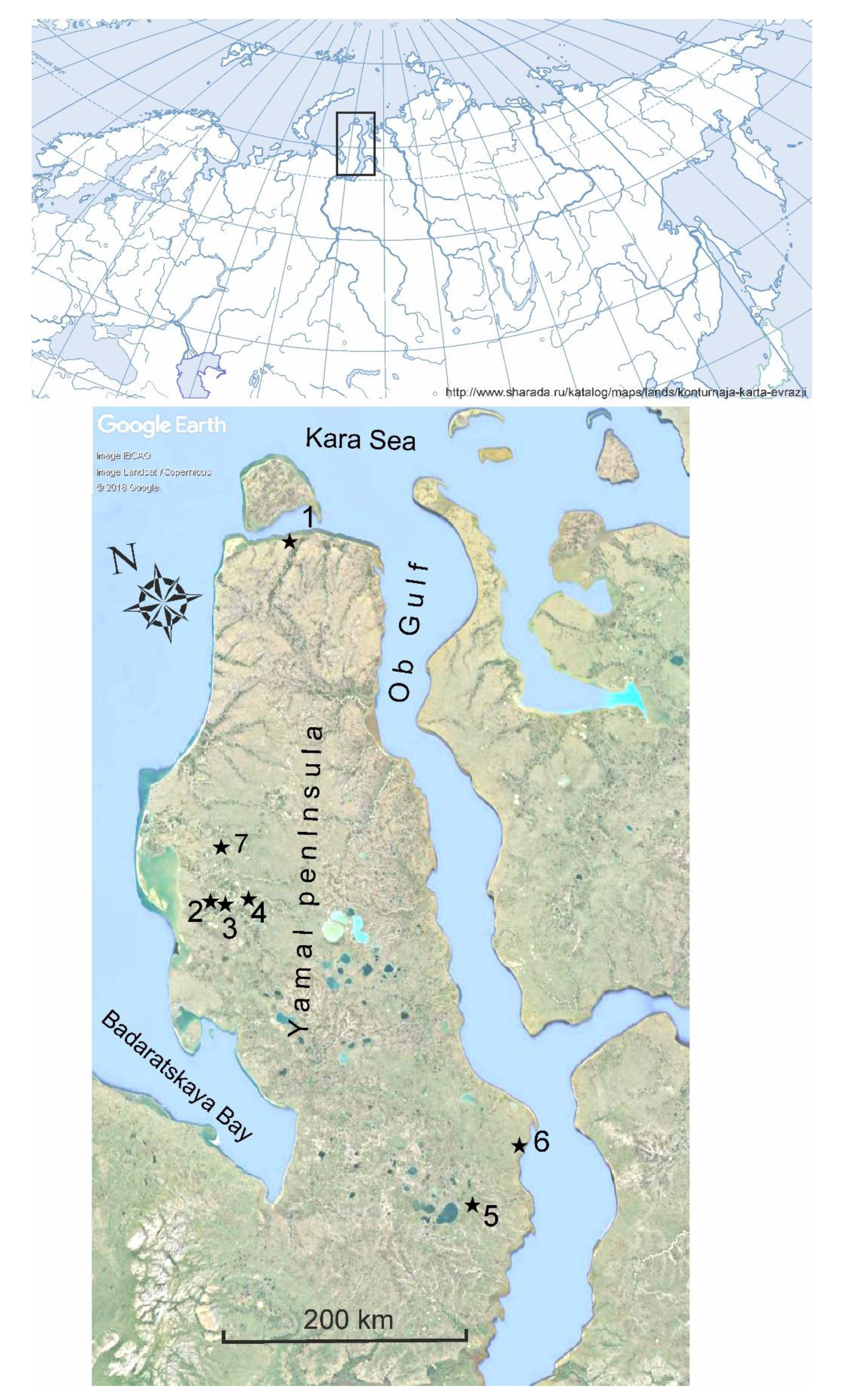
1. Introduction
2. Materials and Methods
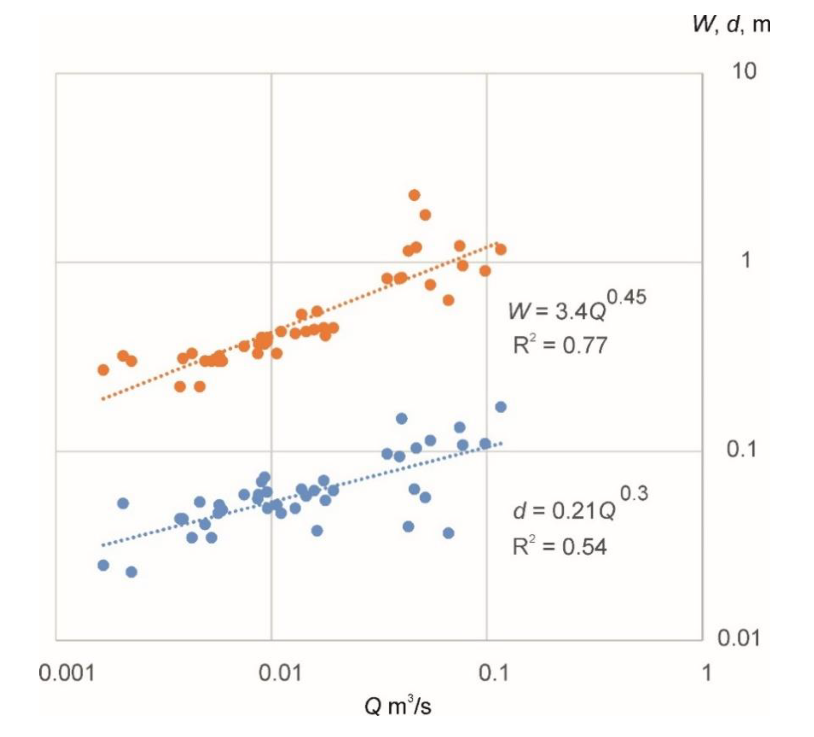
2.1. Theoretical Meanings of Empirical Equations
2.2. The Novel Approach to Erosion Potential Estimation
2.3. Hydrological Modelling
2.4. Model Validation
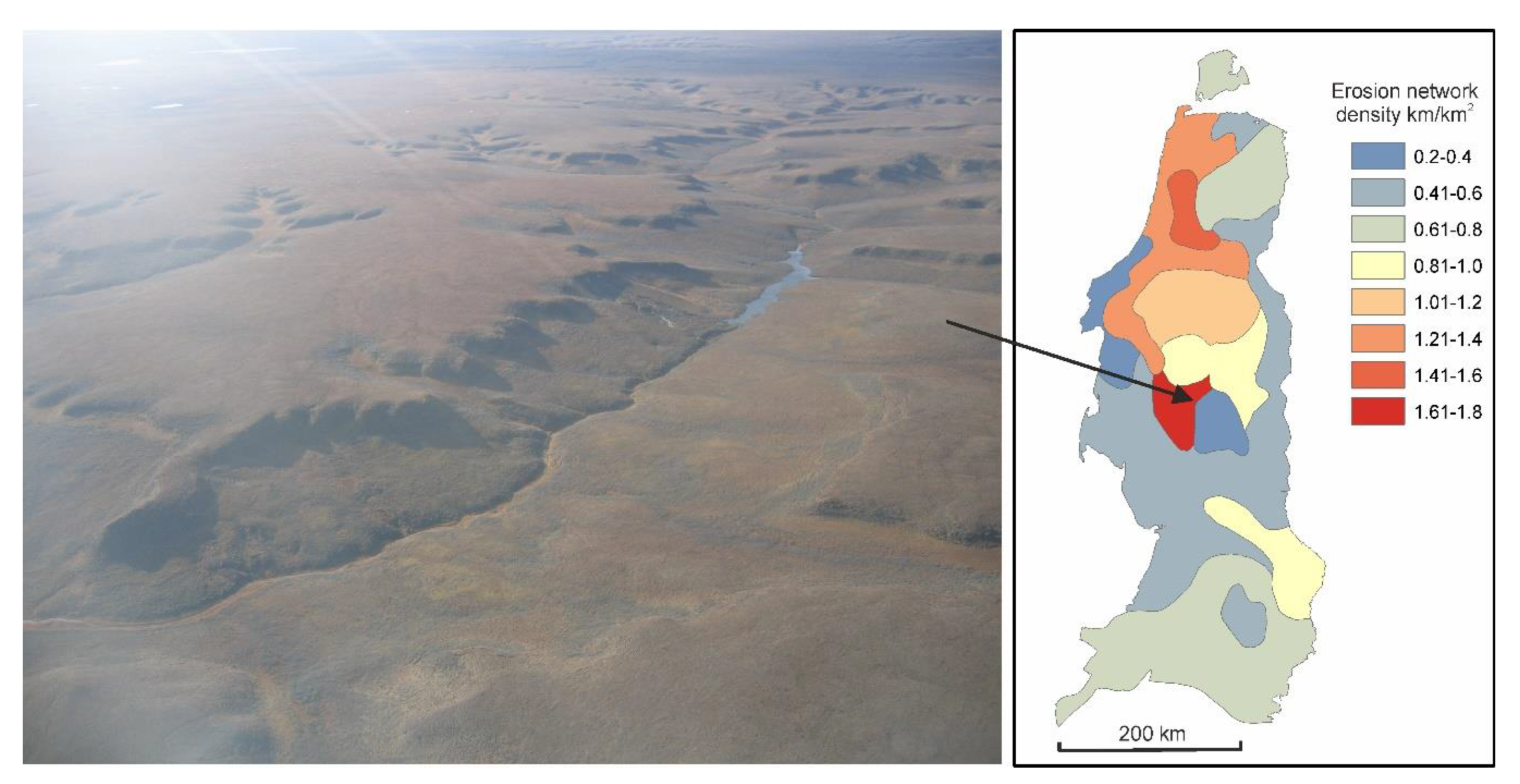
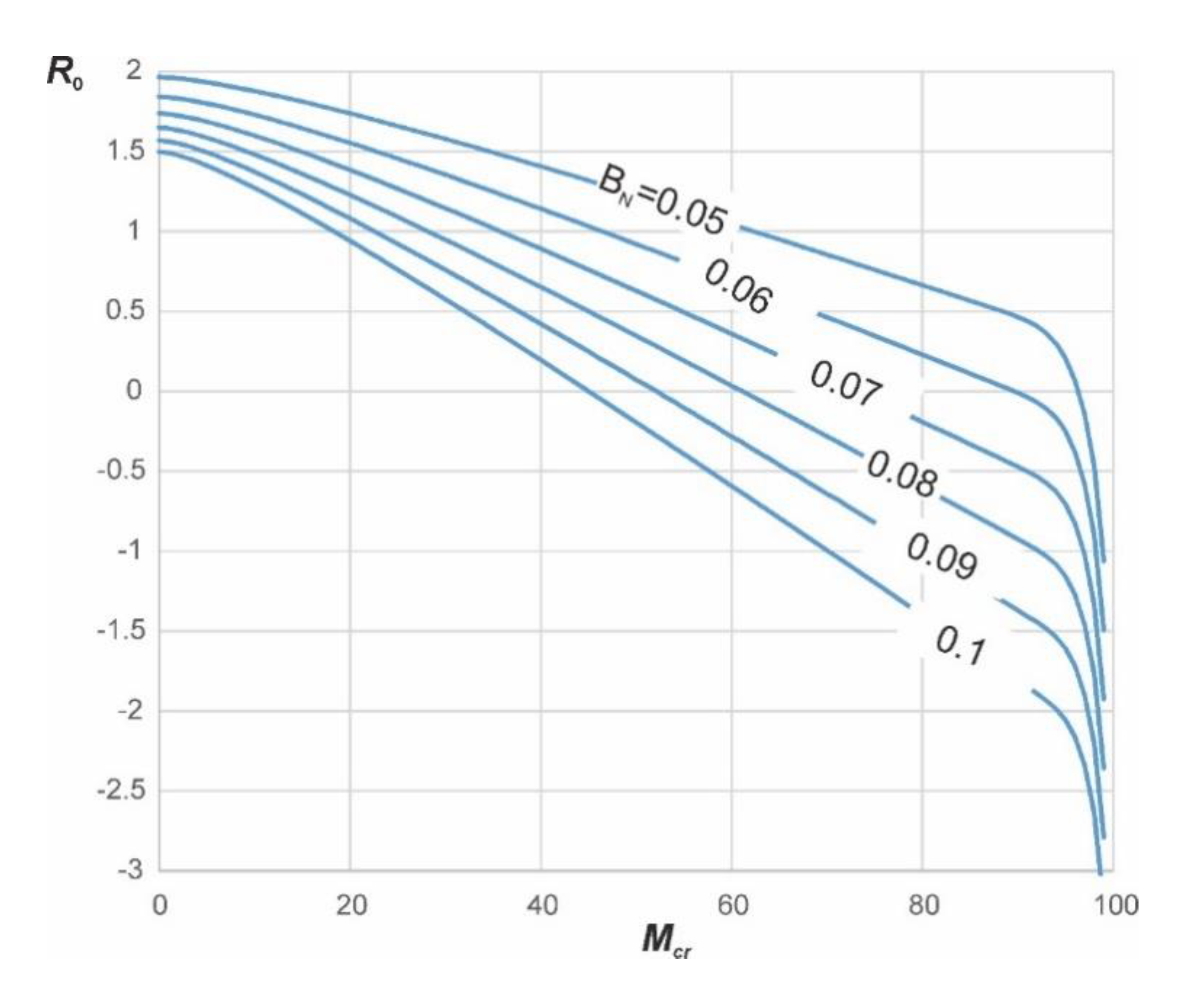
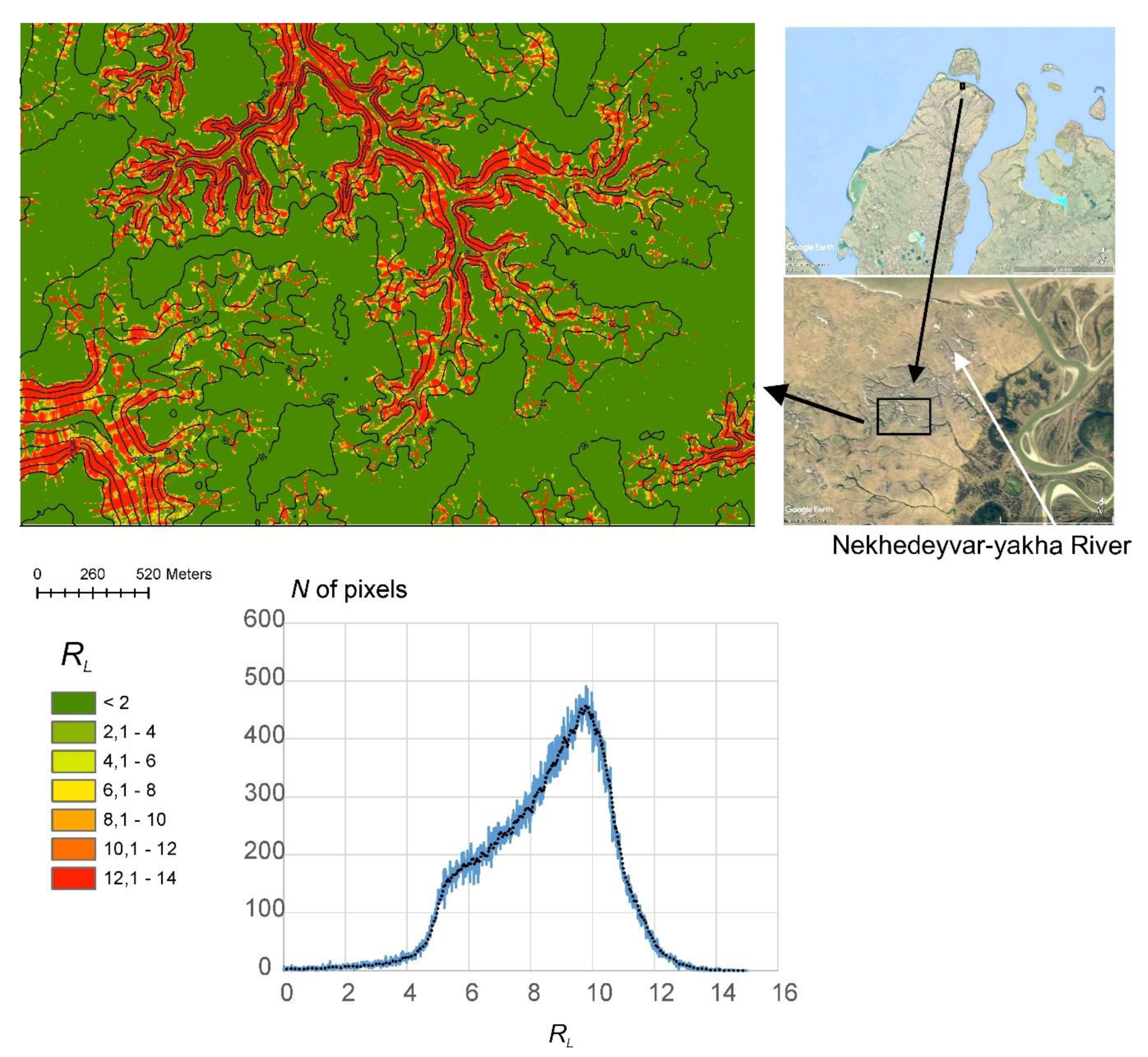
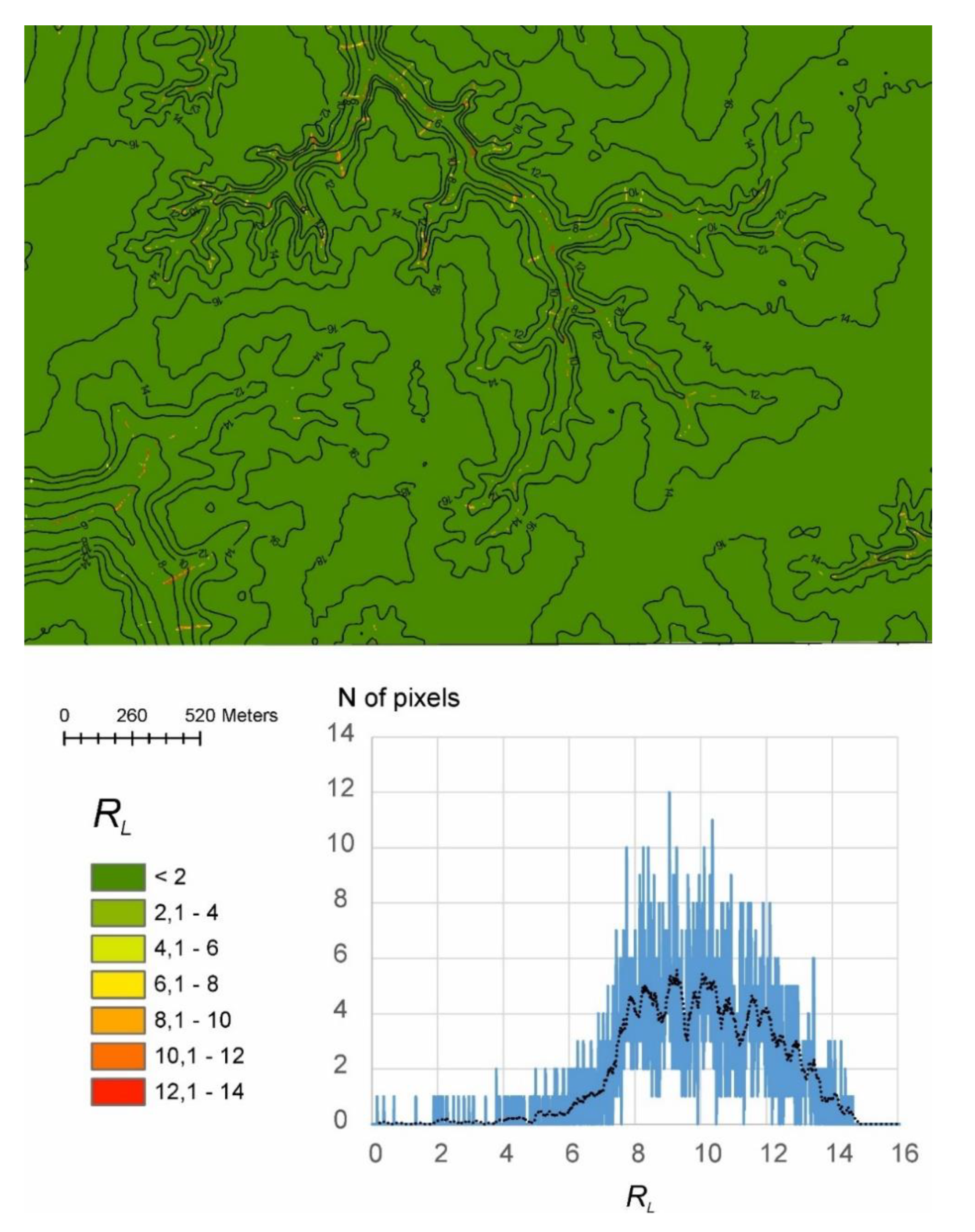
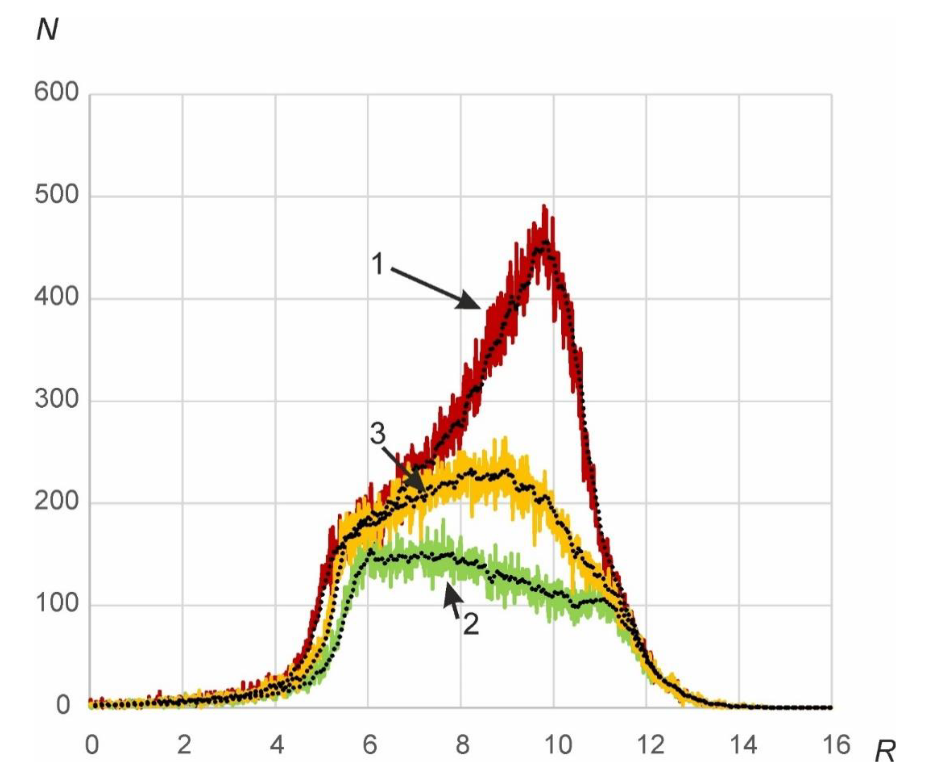
3. Results
4. Discussion
5. Conclusions
Funding
Acknowledgments
Conflicts of Interest
References
- Bennett, S.; Wells, R. Gully erosion processes, disciplinary fragmentation, and technological innovation. Earth Surf. Process. Landf. 2019, 44, 46–53. [Google Scholar] [CrossRef]
- Valentin, C.; Poesen, J.; Li, Y. Gully erosion: Impacts, factors and control. CATENA 2005, 63, 132–153. [Google Scholar] [CrossRef]
- Liu, X.; Li, H.; Zhang, S.; Cruse, R.M.; Zhang, X. Gully Erosion Control Practices in Northeast China: A Review. Sustainability 2019, 11, 5065. [Google Scholar] [CrossRef]
- Carvalho, R.F.; Lopes, P.; Leandro, J.; David, L.M. Numerical Research of Flows into Gullies with Different Outlet Locations. Water 2019, 11, 794. [Google Scholar] [CrossRef]
- Gong, C.; Lei, S.; Bian, Z.; Liu, Y.; Zhang, Z.; Cheng, W. Analysis of the Development of an Erosion Gully in an Open-Pit Coal Mine Dump During a Winter Freeze-Thaw Cycle by Using Low-Cost UAVs. Remote Sens. 2019, 11, 1356. [Google Scholar] [CrossRef]
- Forbes, B.; Stammler, F.; Kumpula, T.; Mysshtyb, M.; Pajunen, A.; Kaarlejärvi, E. High resilience in the Yamal-Nenets social-ecological system, West Siberian Arctic, Russia. Proc. Natl. Acad. Sci. USA 2009, 106, 22041–22048. [Google Scholar] [CrossRef]
- Nature of Yamal (Priroda Yamala); Dobrinski, L.N., Ed.; Nauka: Ekaterinburg, Russia, 1995; p. 435. (In Russian) [Google Scholar]
- Schumm, S.A. Geomorphic thresholds: The concept and its applications. Trans. Inst. Br. Geogr. 1979, 4, 485–515. [Google Scholar] [CrossRef]
- Wolman, M.G.; Miller, J.P. Magnitude and frequency of forces in geomorphic processes. J. Geol. 1960, 68, 54–74. [Google Scholar] [CrossRef]
- Patton, P.C.; Schumm, S.A. Gully erosion, northwestern Colorado: A threshold phenomenon. Geology 1975, 3, 83–90. [Google Scholar] [CrossRef]
- Vandaele, K.; Poesen, J.; Govers, G.; van Wesemael, B. Geomorphic threshold conditions for ephemeral gully incision. Geomorphology 1996, 16, 161–173. [Google Scholar] [CrossRef]
- Desmet, P.J.; Poesen, J.; Govers, G.; Vandaele, K. Importance of slope gradient and contributing area for optimal prediction of the initiation and trajectory of ephemeral gullies. Catena 1999, 37, 377–392. [Google Scholar] [CrossRef]
- Vandekerckhove, L.; Poesen, J.; Oostwoudwijdenes, D.; Nachtergaele, J.; Kosmas, C.; Roxo, M.J.; de Figueiredo, T. Thresholds for gully initiation and sedimentation in Mediterranean Europe. Earth Surf. Process. Landf. 2000, 25, 1201–1220. [Google Scholar] [CrossRef]
- Garrett, K.K.; Wohl, E.E. Climate-invariant area–slope relations in channel heads initiated by surface runoff. Earth Surf. Process. Landf. 2017, 42, 1745–1751. [Google Scholar] [CrossRef]
- Begin, Z.B.; Schumm, S.A. Instability of alluvial valley floor: A method for its assessment. Trans. Am. Soc. Agric. Eng. 1979, 22, 347–350. [Google Scholar] [CrossRef]
- Begin, Z.B.; Schumm, S.A. Gradational thresholds and landscape singularity: Significance for Quaternary studies. Quat. Res. 1984, 21, 267–274. [Google Scholar] [CrossRef]
- Harvey, M.D.; Watson, C.C.; Schumm, S.A. Gully Erosion; Tech. Note 366; U.S. Dep. of the Inter., Bur. of Land Management: Washington, DC, USA, 1985; p. 181.
- Montgomery, D.R.; Dietrich, W.E. Landscape dissection and drainage area-slope thresholds. In Process Models and Theoretical Geomorphology; Kirby, M.J., Ed.; Wiley: New York, NY, USA, 1994; pp. 221–246. [Google Scholar]
- Mirtskhulava, T.Y. Osnovy Fiziki i Mekhaniki Erozii Rusel (Principles of Physics and Mechanics of Channel Erosion); Gidrometeoizdat: Leningrad, Russia, 1988; p. 303. (In Russian) [Google Scholar]
- Zorina, Y.F. Quantitative methods of estimating of gully erosion potential. In Eroziya Pochv i Ruslovyye Protsessy (Soil Erosion and Channel Processes); Chalov, R.S., Ed.; Moscow Univ. Press: Moscow, Russia, 1979; Volume 7, pp. 81–90. (In Russian) [Google Scholar]
- Park, C.C. World-wide variations in hydraulic geometry exponents of stream channels: An analysis and some observations. J. Hydrol. 1977, 33, 133–146. [Google Scholar] [CrossRef]
- Sidorchuk, A. Dynamic and static models of gully erosion. Catena 1999, 37, 401–414. [Google Scholar] [CrossRef]
- Sidorchuk, A. Gully erosion in the cold environment: Risks and hazards. Adv. Environ. Res. 2015, 44, 139–192. [Google Scholar]
- ArcticDEM, 2018. Harvard Data V1. Available online: https://doi.org/10.7910/DVN/OHHUKH (accessed on 28 February 2019).
- Quantum GIS Development Team, 2004–2019. V3.10. Available online: https://qgis.org (accessed on 28 October 2019).
- Sidorchuk, A.; Grigor’ev, V. Soil erosion on the Yamal peninsula (Russian Arctic) due to gas field exploitation. Adv. GeoEcol. 1998, 31, 805–811. [Google Scholar]
- Bobrovitskaya, N.N.; Baranov, A.V.; Vasilenko, N.N.; Zubkova, K.M. Hydrological conditions. In Erosion Processes at the Central Yamal (Erozionnyye Protsessy Tsentral’nogo Yamala); Sidorchuk, A., Baranov, A., Eds.; RNII KPN: St. Petersburg, Russia, 1999; pp. 90–105. (In Russian) [Google Scholar]
- Hydrology of the Wetlands of the Permafrost Zone of Western Siberia (Gidrologiya Zabolochennykh Territoriy Zony Mnogoletney Merzloty Zapadnoy Sibiri); Novikov, S.M., Ed.; VVM Publ. House: St. Petersburg, Russia, 2009; p. 536. (In Russian) [Google Scholar]
- Berrisford, P.; Dee, D.P.; Poli, P.; Brugge, R.; Fielding, M.; Fuentes, M.; Kållberg, P.W.; Kobayashi, S.; Uppala, S.; Simmons, A. The ERA-lnterim archive, Version 2.0. ERA Rep. Ser. 2011, 1, 23. [Google Scholar]
- Komarov, V.D.; Makarova, T.T.; Sinegub, E.S. Calculation of the hydrograph of floods of small lowland rivers based on thaw intensity data. Proc. USSR Hydrometeorol. Cent. 1969, 37, 3–30. (In Russian) [Google Scholar]
- Vinogradov, Y.B. Mathematical Modeling of Flow Formation Processes (Matematicheskoye Modelirovaniye Protsessov Formirovaniya Stoka); Gidrometeoizdat: Leningrad, Russia, 1988; p. 312. (In Russian) [Google Scholar]
- Vinogradov, Y.B.; Vinogradova, T.A.; Zhuravlev, S.A.; Zhuravleva, A.D. Mathematical modeling of hydrographs from the unstudied river basins on the Yamal peninsula. Bull. St. Petersburg State Univ. 2014, 7, 71–81. (In Russian) [Google Scholar]
- Gelfan, A.N. Model of formation of river flow during snowmelt and rain. In Erosion Processes at the Central Yamal (Erozionnyye Protsessy Tsentral’nogo Yamala); Sidorchuk, A., Baranov, A., Eds.; RNII KPN: St. Petersburg, Russia, 1999; pp. 205–225. (In Russian) [Google Scholar]
- Popov, Y.G. Analysis of Lowland River Flow Formation (Analiz Formirovaniya Stoka Ravninnykh Rek); Gidrometeoizdat: Leningrad, Russia, 1956; p. 131. (In Russian) [Google Scholar]
- Schlesinger, S.; Crosbie, R.E.; Gagne, R.E.; Innis, G.S.; Lalwani, C.S.; Loch, J.; Sylvester, R.J.; Wright, R.D.; Kheir, N.; Bartos, D. Terminology for model credibility. Simulation 1979, 32, 103–104. [Google Scholar]
- Voskresenski, K.S.; Golovenko, S.S. Distribution of shallow landslides at the central Yamal. In Erosion Processes at the Central Yamal (Erozionnyye Protsessy Tsentral’nogo Yamala); Sidorchuk, A., Baranov, A., Eds.; RNII KPN: St. Petersburg, Russia, 1999; pp. 133–138. (In Russian) [Google Scholar]
- Vasilevskaya, V.D.; Grigoriev, V.Y.; Sidorchuk, A.Y. Stability of the Northern Soils and Ecosystems to Technogenical Influence. In The Development of the North and Problems of Recultivation, Proceedings of the III International Conference, Sankt-Petersburg, Russia, 27–31 May 1996; Komi NTsUrO RAN: Syktyvkar, Russia, 1997; pp. 208–212. [Google Scholar]
- Gyssels, G.; Poesen, J.; Bochet, E.; Li, Y. Impact of plant roots on the resistance of soils to erosion by water: A review. Progr. Phys. Geogr. 2005, 29, 189–217. [Google Scholar] [CrossRef]


| Catchment | 1 | 2 | 3 | 4 | 5 | 6 | 7 |
|---|---|---|---|---|---|---|---|
| Amax, km2 | 1.54 | 1.14 | 1.77 | 7.32 | 1.34 | 1.57 | 29.55 |
| Mean erosion potential | 0.26 | 0.22 | 0.33 | 0.31 | 0.28 | 0.17 | 0.25 |
| Erosion potential level of maximum probability | 9.7 | 10.04 | 10.35 | 10.16 | 10.2 | 10.16 | 10.03 |
| Mmax, mm | 74 | 97.6 | 97.6 | 107.6 | 114 | 118 | 86.2 |
| AN | 21 | 20.6 | 20.6 | 20.8 | 19.0 | 16.9 | 19.5 |
| BN | 0.084 | 0.074 | 0.074 | 0.073 | 0.051 | 0.058 | 0.075 |
© 2019 by the author. Licensee MDPI, Basel, Switzerland. This article is an open access article distributed under the terms and conditions of the Creative Commons Attribution (CC BY) license (http://creativecommons.org/licenses/by/4.0/).
Share and Cite
Sidorchuk, A. The Potential of Gully Erosion on the Yamal Peninsula, West Siberia. Sustainability 2020, 12, 260. https://doi.org/10.3390/su12010260
Sidorchuk A. The Potential of Gully Erosion on the Yamal Peninsula, West Siberia. Sustainability. 2020; 12(1):260. https://doi.org/10.3390/su12010260
Chicago/Turabian StyleSidorchuk, Aleksey. 2020. "The Potential of Gully Erosion on the Yamal Peninsula, West Siberia" Sustainability 12, no. 1: 260. https://doi.org/10.3390/su12010260
APA StyleSidorchuk, A. (2020). The Potential of Gully Erosion on the Yamal Peninsula, West Siberia. Sustainability, 12(1), 260. https://doi.org/10.3390/su12010260