A Comparison of Machine Learning Methods for the Prediction of Traffic Speed in Urban Places

Abstract

Rising interest in the field of Intelligent Transportation Systems combined with the increased availability of collected data allows the study of different methods for prevention of traffic congestion in cities. A common need in all of these methods is the use of traffic predictions for supporting planning and operation of the traffic lights and traffic management schemes. This paper focuses on comparing the forecasting effectiveness of three machine learning models, namely Random Forests, Support Vector Regression, and Multilayer Perceptron—in addition to Multiple Linear Regression—using probe data collected from the road network of Thessaloniki, Greece. The comparison was conducted with multiple tests clustered in three types of scenarios. The first scenario tests the algorithms on specific randomly selected dates on different randomly selected roads. The second scenario tests the algorithms on randomly selected roads over eight consecutive 15 min intervals; the third scenario tests the algorithms on random roads for the duration of a whole day. The experimental results show that while the Support Vector Regression model performs best at stable conditions with minor variations, the Multilayer Perceptron model adapts better to circumstances with greater variations, in addition to having the most near-zero errors.

1. Introduction

In recent decades, cities have become more crowded and jammed, which has increased the need for accurate traffic and mobility management [1] through the development of solutions based on Intelligent Transport Systems. Adaptive traffic lights rely heavily on real-time measurements made by cameras and loops, as well as on the prediction capabilities applied to historical datasets, allowing better accommodation of the traffic flow. Traffic management strategies are applied based on a set of triggers generated by the measurements, so having the capability to predict the activation of these triggers will allow traffic managers to be proactive and apply the right traffic management plan to tackle the traffic congestion before it appears, while the network still has the capacity to efficiently manage it. Therefore, there is a rising interest in short-term forecasting of traffic flow and speed [2], which allows for better regulation of road traffic [3]. The accuracy of estimations and predictions has risen significantly through the use of more granulated data sources [4] and by using different machine learning methods, which are consistently improving prediction performance. The main issue for the prediction of traffic flow in road networks involves the development of an algorithm that will combine computational speed and accuracy for both short-term and long-term problems.

In the literature, various ways of performing short term predictions have been introduced—such as regression models [5], the nearest neighbor method (k-NN) [6], the Autoregressive Integrated Moving Average (ARIMA) [7], and the discretization modeling approach—as easier solutions to the complicated nonlinear models [8], in addition to machine learning algorithms such as Support Vector Regression (SVR) [9,10], Random Forest (RF) [11] for regression, and Neural Networks (NN) [9,11,12]. In [13], a variety of parametric and non-parametric models that were found in literature were compared. Neural Networks, SVR, and Random Forest are some of the most commonly used non-parametric models; however, no single best method that could predict traffic accurately in any situation was proposed. The SVR method has been proven to outperform naïve methods such as Historical Averages [14]. In other studies, the linear regression model has been shown to outperform other models, such as k-NN and kernel smoothing methods [15], in the analysis of traffic speed data.

In [16,17], deep learning approaches performed better than classic machine learning methods such as SVR and ARIMA, but were not compared in terms of predicting traffic speed. In another study, the performances of five different regression models were compared using the Mean Absolute Errors (MAE) of traffic volume with the M5P—an improved version of classification and regression trees [18,19,20]—performing best among the Linear Regression, Sequential Minimal Optimization (SMO) Regression, Multilayer Perceptron, and Random Forest models [21]. The short-term traffic volume prediction ability of the k-NN, SVR, and time series models has been assessed in two case studies in [22], showing that the territory of interest plays a key role when predicting speed. There are also other studies, such as [23,24,25,26], showing that the prediction accuracy of Neural Networks and SVR is better than that of other machine learning models for short-term traffic speed prediction.

This paper focuses on comparing four machine learning algorithms—Neural Networks, Support Vector Regression, Random Forests and Multiple Linear Regression—in terms of predicting traffic speed in urban areas based on historical statistical measures of traffic flow and speed. The data were extracted from and applied to the roads of the city of Thessaloniki, Greece.

The paper is structured as follows. Section 2 deals with the methodological approach and its application to the traffic status in Thessaloniki, and Section 3 reports the effectiveness of the algorithms’ forecasting abilities, assessed in three short-term scenarios. Finally, conclusions and discussion are presented in Section 4.

2. Methodological Approach

2.1. Overview

The main scope is the comparison of four machine learning algorithms—Neural Networks, Support Vector Regression, Random Forests, and Multiple Linear Regression—that will predict the traffic status in the city of Thessaloniki. In this section, we describe the data we collected from the streets of Thessaloniki, the pre-processing steps, and the features that comprise the training data, as well as the machine learning models, their optimization, and the evaluation metrics, as shown in Figure 1.

2.2. Data Collection

The city of Thessaloniki is the second largest city of Greece and the largest city of Northern Greece. Its population amounts to more than 1 million citizens in its greater area, which covers 1500 km${}^2$. It has an average density of 665 inhabitants per km${}^2$ [27]. The mobility data sources in Thessaloniki include conventional traffic data sources, such as traffic radars, cameras, and loops, as well as probe data, both stationary and from the bluetooth detector network of the city and Floating Car Data (FCD), which were acquired from a 1200 taxi fleet [28].

Therefore, the data used for this study are a subset of the FCD generated by half of the taxi fleet in Thessaloniki, containing location (GNSS), orientation, and speed. This data was aggregated in 15 min intervals for each road segment, generating a distribution of speeds of the different taxis that circulated through each road segment during the last 15 min. More concretely, the dataset was composed of 5 months of traffic data per road segment and various indicators of the speed for every 15 min; these are presented in Section 2.3.

We decided to use only internal factors, as the inputs to our models consisted of traffic data along with statistical measures of road speed. The aim was to build data-driven models which will predict any changes that could affect the traffic flow, i.e., a heavy rain or some social or athletic event, without having any information about it.

An example of the distribution of the FCD records for every 15 min over a period of 2 weeks is shown in Figure 2. A peak was observed before midday every day, which was reduced slowly after midday. In addition, there was a significant reduction on weekends (2–3 March, 2019 and 9–10 March, 2019) and public holidays (11 March, 2019 was Clean Monday, which is a public holiday in Greece and Cyprus).

2.3. Pre-Processing and Training

The collected data were then processed by using the TrafficBDE package [29] of the R Project for Statistical Computing [30] in RStudio Integrated Development Environment (IDE) [31]. We calculated and scaled the following road data between 0 and 1: Minimum, maximum, standard deviation, mean, skewness and kurtosis of speed at the 15 min time window, the date and time at which they were observed, the entries of the road, and the unique entries. These measures were the training inputs of RF, SVR, NN, and LR models. These models were trained with data from the two weeks previous to the desired date time, which amounted to a total of 1344 quarters. If any missing values of these measures existed in any time period, they were filled via linear interpolation. Next, each of the RF, SVR, NN, and LR model families was trained and optimized via 10-fold cross validation; however, this process is time consuming for real-time predictions with big data. Multiple and different models for each model family were tested on training results. The advantage of this process is that the model with the lowest Root Mean Square Error (RMSE) will be selected to predict the mean speed of the requested date and time [12]. For example, at a given date and time, multiple NN models with different layers were tested and the model with the best accuracy was selected to predict the mean speed. This training process was applied to all four models.

2.4. Random Forest

A Random Forest (RF) is an ensemble technique which can perform regression tasks by growing multiple decision trees and combining them with Bootstrap Aggregation, broadly known as bagging. First, the number of trees $n_{tree}$ and bootstrap samples are drawn from the training set data. For each sample, a regression tree is fully grown, with the modification that at each node, rather than choosing the best split among all predictors, a random sample $m_{try}$ of the predictors is chosen and the best split is determined from those variables. The prediction of the mean speed is obtained by aggregating the predictions of the $n_{tree}$ trees, i.e., averaging the predictions [32].

In order to implement an RF, two R packages were used—caret [33] and randomForest [34]. By using the training set data and performing 10-fold cross-validation, the best combination of the number of trees ($n_{tree}$) and the number of variables available for splitting at each tree node ($m_{try}$) were selected; the best model was trained and was used to predict the speed in the test set. The RF builds multiple decision trees and averages their predictions (Figure 3). Despite the high variance each tree might have, the entire forest will have lower variance and, therefore, the predictions of the speed will be more accurate and stable.

2.5. Support Vector Regression

Support Vector Regression (SVR) is an adaptation of the SVM (Support Vector Machine) algorithm used for regression problems. Support vector regression is a generalization of a simple and intuitive classifier called the maximal margin classifier. SVR uses a type of loss function called $\epsilon$-insensitive, where if the predicted value is within a distance epsilon from the actual value, there is no penalty in the training loss function. The parameter $\epsilon$ affects the number of support vectors used in the regression function, i.e., the smaller the value of $\epsilon$ is, the greater the number of support vectors that will be selected. Another important parameter of the SVR model—as it affects both its performance and complexity—is the cost parameter (C), which determines the tolerance of deviations larger than $\epsilon$ from the real value; i.e., smaller deviations are tolerable for larger values of C [35]. Another important aspect of SVR is the ability to model nonlinearity with polynomials of the input features or other kernel functions [36]. This allows us to efficiently expand the feature space with the goal of achieving an approximate linear separation. A kernel parameter gamma ($\gamma$) is introduced by the kernel we used, which is the radial basis function:

$$K(x_i,x_j)=exp(-\gamma ||x_i-x_j{\left|\right|}^2).$$

The gamma parameter, which is the inverse of the standard deviation, controls the radius of influence of the support vectors, with high values of gamma resulting in the area of influence of the support vectors including only the support vector itself. All three parameters of the SVR model affect its complexity and performance. In order to implement the SVR model, the e1071 package was used [37]. Many combinations of the values of the cost, the epsilon, and the gamma parameters were evaluated by performing 10-fold cross-validation with the use of the training set in order to optimize and determine the best model. When the best parameters were determined, an SVR model with radial kernel was trained in order to make the prediction of the mean speed on the test set.

2.6. Multilayer Perceptron

Multilayer perceptron (MLP) [38] is a feedforward Artificial Neural Network (ANN) model that can deal with non-linearity. MLP consists of a number of layers: The input layer, hidden layers, and the output layer. The input layer, which consists of seven nodes, receives the inputs, which are then moved forward through the MLP by taking the dot product of each layer with the weights of the following layer. This dot product results in some values that are then passed through an activation function—specifically, the logistic activation function—for all the layers except the output where the linear activation function is applied. The process is repeated for the next layers until it reaches the output layer that consists of one node; that is the predicted value of the mean speed. Each layer is fully connected to the next one. During the training process of the model, i.e., the updating of the weights, the output is compared to the real value and an error is calculated. This error is then propagated back through the network with the use of the resilient back propagation (Rprop) algorithm, which is often faster than training with back propagation and focuses on eliminating the influence of the size of the partial derivative on the weight step. Therefore, only the sign of the derivative is considered for the indication of the direction of the weight update; the updated value determines the size of the weight change [11]. The TrafficBDE package was used in order to build and train the appropriate MLP models [29]. By using 10-fold cross-validation, different combinations of the number of neurons in each hidden layer are tested in order to select the model with the lowest error and train it to predict the mean speed (Figure 4).

2.7. Multiple Linear Regression

Linear regression is a parametric model and a supervised learning algorithm which uses a linear approach for a prediction problem [39]. In linear regression, the prediction function is assumed to be a linear combination of the features. It tries to fit a line that explains the relationship between the independent variable and the dependent variable(s) [13].

$$y_i={\beta }_0+{\beta }_1{x}_{i1}+{\beta }_2{x}_{i2}+\cdots +{\beta }_p{x}_{i7}+\epsilon$$

where, for $i=n$ observations and $j=1,\cdots ,7$ independent variables, $y_i=$ dependent variables, $x_i=$ independent variables, ${\beta }_0=$ constant term, ${\beta }_p=$ slope coefficients for each independent variable, and $\epsilon =$ the model’s error term.

In our case, the independent variable is the mean speed and the dependent variables are the minimum, maximum, standard deviation, skewness, kurtosis of speed, car entries, and unique car entries. Although the model is simple, in some cases, it is shown to produce quite good results, as well as very fast predictions due to its simple form.

2.8. Measuring Prediction Accuracy

In order to assess the quality of the traffic predictions, it is essential to establish metrics that allow the comparison of the different methods. This evaluation must consist of a comparison between the traffic prediction results and the actual traffic conditions at the selected date and time. We used the following metrics:

• Mean Absolute Error (MAE)—This metric corresponds to the average absolute difference between the predicted $\widehat{y}$ and the true values y [40].

  $$MAE=\frac{1}{n}\sum _{j=1}^n|y_j-\widehat{y_j}|.$$
• Root Mean Square Error (RMSE)—This metric corresponds to the square root of the mean of the squared difference between the observed y and the predicted values $\widehat{y}$.

  $$RMSE=\sqrt{\frac{1}{n}\sum _{j=1}^n{(y_j-\widehat{y_j})}^2}.$$

These metrics were used in three evaluation scenarios, described in Section 3, which will evaluate the models’ performances from different perspectives.

3. Results

The effectiveness of the algorithms’ forecasting abilities was assessed via multiple comparisons in three scenarios:

• Speed prediction at random dates and times on randomly selected roads.
• Speed prediction on randomly selected roads, at eight consecutive dates and times.
• Speed prediction on randomly selected roads for the duration of a specific 24 h time window.

It is observed in Figure 2 that there are patterns in traffic flow. The first scenario is based on random tests from 1 January, 2019 to 31 May, 2019. The scenario of “speed prediction at randomly selected roads, at eight consecutive dates and times” aims to show which family of models follows the patterns observed at specific times—e.g., traffic during working hours. The last scenario focuses not only on the prediction accuracy but also on the robustness of these models. We are interested in robust models that adapt to abrupt changes in the traffic flow due to exogenous conditions such as socio-demographics, income development, migration, oil prices, economic growth, and weather-induced network deterioration.

3.1. Speed Predictions at Random Dates and Times on Random Roads

In the first scenario, multiple predictions at different and random dates and times between January and May 2019 and on random roads were made using each of four models. Figure 5 shows the RMSEs for all models.

As can be seen in

Table 1. Mean Absolute Error (MAE) of one random date and time at randomly selected roads.

SVR	NN	RF	LR
6.25	6.57	6.44	6.90

, since the MAE expresses the average model prediction error in units of the roads’ mean speeds (km/h), it is observed that the average error of the 35 tests for all models is approximately the same as that of the SVR model—about 0.2 km/h more accurate than the RF and NN models. The high interquartile range (IQR) of the RF model suggests that the errors are more scattered compared to those of SVR and NN models. The LR model’s lower quartile is higher than the others, which suggests that the errors are more concentrated and there are fewer small errors as compared to the other models.

3.2. Speed Prediction at Eight Consecutive and Random Dates and Times on Random Roads

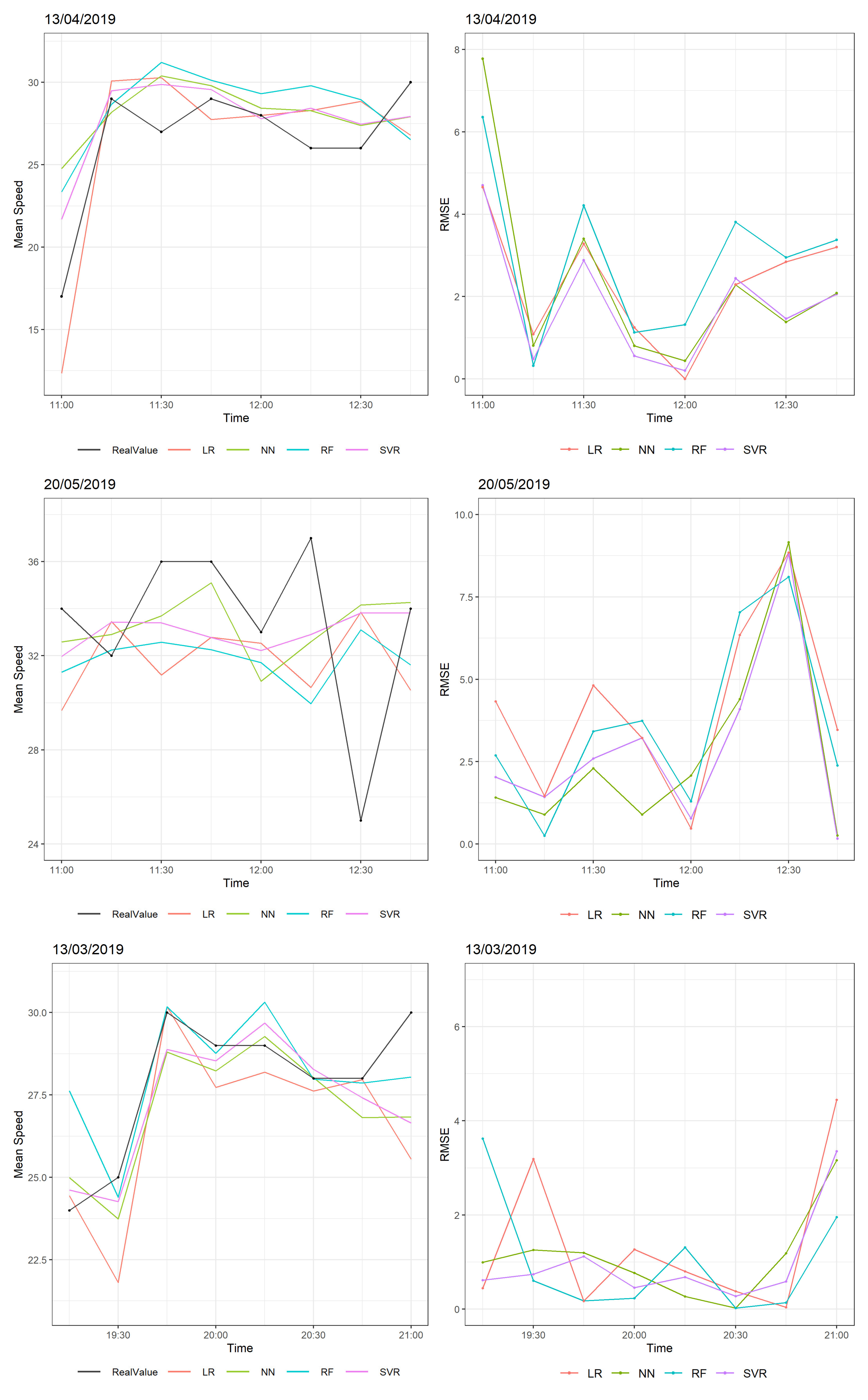
Next, we predicted speeds at eight consecutive and random quarters on random roads. The selected dates were from weekdays and weekends, and the times were mostly working hours—e.g., 9:00 a.m. when people commute to their jobs, 11:00 a.m. when the shops are open, at 7:00 p.m. when people get home from their jobs, and even later in the evening. During those hours, the street activity is higher; that is when a good prediction might be necessary.

Figure 6 shows the RMSE of the four models. In this scenario, there was one abrupt change in speed at the start, middle, and end of the examined two hour time. Large RMSE values occurred at 13 April 2019 and at 20 May 2019, where there was an abrupt change in average speed of around 10–15 km/h. All models tried to follow this change, achieving RMSE values at 5–8 km/h, which is large considering that the other predictions of these time windows have RMSEs less than 4 km/h. However, on 13 March 2019, all models performed better with a change of speed at 5 km/h where the RMSE was less than 4 km/h. Specifically, in most cases, the Neural Network and SVR models performed better in terms of RMSE, and the linear regression model was often influenced by abrupt changes, leading to greater error.

3.3. Speed Prediction on Random Days and on Random Roads

Building models that are robust to abrupt changes in traffic flow caused by various reasons, such as social events or heavy weather events, is of great interest. In this scenario, we predicted average speeds on random days and on random roads, in order to determine the model which performs better and adapts to the changes in traffic flow during the day. Two days are presented below: One day without large changes and one with large changes in traffic flow.

Figure 7 shows the traffic speed distribution of one random road on 27 February, 2019, when there were frequent and abrupt changes of speed. Before 06:00, average speed levels fluctuated between 40–50 km/h; the models tried to follow the changes in speed. LR and RF had RMSEs of almost 15 km/h. After 6:00 a.m., the average speed decreased by 20–30 km/h, meaning that there was an increasing number of cars in this road. At this time, all models had their maximum RMSEs, which were around 15 km/h. For the rest of the day, LR and RF had large RMSE values when there were large and abrupt deviations in speed, whereas NN and SVR showed better performance with the minimum MAE and RMSE values and the minimum of maximum errors, as shown in

Table 2. MAE, RMSE, and maximum error of the models’ predictions on 27 February 2019.

Model	MAE	RMSE	Max Error
NN	3.74	5.90	29.81
SVR	3.67	5.49	31.25
RF	3.87	5.90	32.99
LR	4.10	6.10	34.65

.

Figure 8 shows the traffic speed distribution of another random road on 13 March 2019 when there were fewer abrupt changes than in the previous Figure. Early in the morning, two large decreases in speed were observed: From 45 to 20 km/h and from 45 to 10 km/h. All models performed their maximum RMSE values at these time points. For the rest of the day, all models had small RMSE values, with NN and SVR performing better in terms of MAE and RMSE, as is shown in

Table 3. MAE, RMSE, and Maximum Error of the models’ predictions on 13 March 2019.

Model	MAE	RMSE	Max Error
NN	4.22	5.36	15.17
SVR	4.30	5.40	14.97
RF	4.71	5.76	15.88
LR	4.59	5.79	17.97

. Generally, all models follow the traffic pattern and recognize the changes of speed, but when an abrupt change of traffic flow occurs, NN and SVR models seem to follow the large deviations; the larger the abrupt change in speed, the larger error for the LR and RF models.

4. Discussion and Conclusions

A comparison of neural networks, support vector machines, random forests, and multiple linear regression was implemented for predicting the traffic status of Thessaloniki.

The data were collected by stationary and floating traffic data sources generating a large database that spatially and temporally covered the city. We summarized these data in time windows of 15 min. We extracted the minimum, maximum, standard deviation, mean, skewness and kurtosis of speed, and the frequency of the unique cars that entered each road; we normalized and used them as the training features in machine learning algorithms to predict mean speeds. The best parameters of each model were determined via 10-fold cross validation. Using 10-fold cross validation, the training set was separated into 10 equal datasets; nine of them were used to train the RF, SVR, and NN and to predict the requested mean speed. This process was repeated 10 times; according to the smallest error, the RF, SVR, and NN were chosen. Through this process, the optimal combination of trees and the number of variables for splitting at each tree node were evaluated in RF; multiple combinations of cost, epsilon, and gamma parameters were tested with the radial kernel in SVR, and multiple combinations of neurons and layers were tested in MLP. The benefit of this process, even though it is time consuming in real-time prediction, is that the model with the lowest RMSE will be selected to predict the mean speed at a given date and time.

The evaluation process was divided into three scenarios: Speed prediction at one random date and time on randomly selected roads, speed prediction on randomly selected roads at eight consecutive dates and times, and speed prediction on randomly selected roads for the duration of a 24 h period. As shown in Figure 2, there are daily and weekly patterns in traffic flow. These scenarios focus not only on the prediction accuracy, but also on the robustness of the tested models. There is a need for robust models that can adapt to large changes in traffic flow. In the first scenario, we predicted speed at 35 random dates and times between January and May 2019 on random roads. The median RMSE of these results was between 6–7 km/h for all models, with SVM performing better than the other models. The RF and LR were efficient when the pattern of mean speed was almost linear; when an abrupt change in traffic occurred, these models had large RMSE values. The RMSEs of the RF were more scattered compared to those of SVR and NN models, as shown in Figure 5; the LR model’s lower quartile is higher than the others, which suggests that the errors were more concentrated and that there were fewer small errors as compared to the other models. In the next scenario, we predicted speed within two hours at three times and on three random roads. The selected times were working hours and hours when people would get home from work. The minimum RMSE values occurred in the NN and SVM models indicating, that these models were more capable of following abrupt changes in speed. In the last scenario, we predicted speed on two roads of Thessaloniki for 24 h on two random roads. We observed that large deviations of speed make the LR and RF models less accurate than the NN and SVR models. The NN model adapted and predicted in a better way for larger traffic flow changes, while the SVR model had a better accuracy during the periods of smaller changes. The NN model also had the most near-zero errors in its predictions compared to the other three models. The NN and SVR models performed on both linear and non linear patterns. The RF model mostly resulted in medium-sized errors compared to the other models, while the LR model, if heavily influenced by traffic changes, led to higher errors.

The future work of the authors will examine the patterns of speed within the city depending on the location of the road, the date, and the time in order to select and use the appropriate machine learning model to achieve better accuracy in real time speed predictions. Moreover, the authors will deal with optimizing and comparing other algorithms which have been studied, as well as more classical methods and parametric models. Finally, testing of the models developed in this paper in other cities is of great interest, as well as combining these data with external data, such as weather data, using linked data technology. The handicap in using external data is that the resolution of weather prediction data is usually lower (1–3 h), which may be ok for other uses (e.g., estimating demand for bike-sharing services), but is not enough for traffic status prediction. In this case, the reaction of traffic to adverse weather conditions is composed first of a larger number of vehicles in the street (which can be tackled in the 3 h interval), but also has an instantaneous effect by reducing the capacity of the streets and speeds overall, so the efficient addition of this data is the next challenge on which the research team is working.