Spatial Heterogeneity of Winter Wheat Yield and Its Determinants in the Yellow River Delta, China

Abstract

Understanding spatial differences of crop yields and quantitatively exploring the relationship between crop yields and influencing factors are of great significance in increasing regional crop yields, promoting sustainable development of regional agriculture and ensuring regional food security. This study investigates spatial heterogeneity of winter wheat yield and its determinants in the Yellow River Delta (YRD) region. The spatial pattern of winter wheat in 2015 was mapped through time series similarity analysis. Winter wheat yield was estimated by integrating phenological information into yield model, and cross-validation was performed using actual yield data. The geographical detector method was used to analyze determinants influencing winter wheat yield. This study concluded that the overall classification accuracy for winter wheat is 88.09%. The estimated yield agreed with actual yield, with R² value of 0.74 and root mean square error (RMSE) of 1.02 t ha⁻¹. Cumulative temperature, soil salinity and their interactions were key determinants affecting winter wheat yield. Several measures are recommended to ensure sustainable crop production in the YRD region, including improving irrigation and drainage systems to reduce soil salinity, selecting salt-tolerant winter wheat varieties, and improving agronomy techniques to extend effective cumulative temperature.

1. Introduction

Agricultural production is a critical issue related to food security guarantee, regional economic development and social stability for local government [1,2,3]. Approximately 14.29% of the global land-surface area is covered by cultivated land [4]. Due to limited cultivated land resources and continued population growth, global agricultural production faces enormous challenges. Owing to continuously growing population from seven billion in 2010 to nine billion in 2050 and limited land resources, a global food gap will appear [5]. To fill the yield gap between supply and demand, it is imperative to increase crop yield. Affected by internal and external factors, the crop growth and its ultimate yield usually involve complex procedures, which have a significant spatial heterogeneity [6,7,8,9,10]. Hence, identifying spatial heterogeneity of crop yields, determining the influencing factors and quantifying theirs effects on crop yield are of great significance for improving crop yield and achieving sustainable development of agriculture.

As important research fields in precision agriculture, accurate crop identification and yield estimation are preconditions for studying spatial heterogeneity of crop yields and their determinants [11]. Commonly depending on crop acreage, yield estimation is an important basis for establishing agriculture policy. Traditionally, crop condition has been estimated through national census and household surveys, which is collected in situ with low temporal and spatial resolution. Monitoring crop condition over large area through traditional methods, however, is time consuming and costly, owing to the spatial heterogeneity in soil characteristics, nutrition status, crop variety and so on [12]. With development of satellite technology, remote sensing has been widely applied in regional crop condition monitoring since the 1970s [13,14,15,16,17,18]. Remote sensing provides a cost-effective and timely way to monitor crop condition than traditional survey procedures [1]. Among remote sensing data, moderate resolution imaging spectroradiometer (MODIS) exhibits excellent temporal resolution and medium spatial resolution, thus making it suitable for crop condition monitoring and estimation at large scale [18,19]. Many studies have proved the efficiency of MODIS data in crop mapping, yield estimation and forecasting over large areas [20,21,22,23].

Crop classification through remote sensing approaches has gone through four stages [24], covering the traditional unsupervised and supervised classification method [25,26], the intelligent classifier method [27,28], the time series similarity analysis method [29,30] and the phenology-based identification method [31,32,33,34]. Among these approaches, time-series similarity analysis is widely used in cropland mapping, which could depict the characteristics of crop profiles. Different time series similarity analysis methods have been applied to map crop types, such as Minkowski distance (e.g., Euclidean distance and Mahalanobis distance), time-series match distance (Dynamic Time Warping (DTW) and Longest Common Sub-Sequence (LCSS)) [35], and time series similarity method combined with transform approach (e.g., Fourier transform and Principal Component Analysis (PCA)). Wang et al. [36] evaluated the performance of Minkowski distance and DTW distance, both of which achieved a relatively good result. Zhang and Kinsner [37] believed that the DTW algorithm is too slow to be practical and the computing cost is relatively high. As the most widely used method, Minkowski distance can obtain high matching accuracy, which have generated encouraging results for large-area crop mapping as well as winter wheat classification with success [38,39].

Based on crop acreage acquisition, studies have been applied to evaluate crop yield at the regional level by using remote sensing technology [40,41]. Methods for regional yield estimation are mainly divided into two categories. One is a statistical empirical model or a descriptive model, that is, using statistical methods such as regression analysis and correlation analysis to describe the relationship between crop yield and parameters derived from remotely sensed data (e.g., Normalized Difference Vegetation index (NDVI) and Leaf Area Index (LAI)), which assumes that spectral data are correlated with canopy reflectance parameters and ultimate yield. [42]. The other is the kinetic model or explanatory model, such as the crop growth model [43,44]. Both two yield estimation methods have been successfully applied at regional scale. Dente et al. [45] assimilated leaf area index into Crop Estimation through Resource and Environment Synthesis (CERES) crop growth model to predict wheat yield at catchment scale. Ren et al. [46] accurately estimated wheat yield by establishing relationships between LAI and wheat yield at the main growth stage. Compared with crop growth models with complex mechanisms, the regression model is the most common quantitative analysis approach, which requires fewer input parameters and parameters are easier to obtain [47]. Due to the advantage of short revisit period and medium spatial resolution, MODIS is widely used for yield estimation based on time series analysis. Kouadio et al. [48] assessed regional wheat yield based on features of the Green Area Index (GAI) derived from time series MODIS data. Based on years of MODIS images, Bognár et al. [49] estimated and forecasted wheat yield. Many researches indicate that the accuracy of crop yield estimation can be improved by integrating phenological metrics [50,51,52,53].

Evidence from many studies proves that crop yield determined by many factors, such as climate [6], elevation and terrain attributes [7,8], soil properties [9,10,11] and human activity [10]. To explore the relationship between crop yield and influencing factors, most of the existing studies have been conducted qualitatively by using traditional method, such as controlled trial and variable-controlling approach [54,55,56,57]. However, the comprehensive comparisons between factors and variable combinations are still lacking and the contribution rate of multi-factor effects and their interactions cannot be effectively quantified through traditional method. Moreover, the observation scale of traditional method is relatively small, mainly focusing on field scale [58]. Actually, crop yield and its influencing factors have significant spatial variability at large scale, which was not considered in traditional methods. As a new statistical method, the geographical detector is developed to detect spatial heterogeneity and explore its driving forces [59]. The geographical detector method is implemented based on the assumption that if an independent variable has a significant impact on a dependent variable, the spatial pattern of independent variable and the dependent variable should be similar [60]. The method has been widely used in social sciences [61,62], human health [63,64], natural sciences [65] and environmental sciences [66,67] etc.

To better explain the spatial variance in crop yield linked to influencing factors, it is important to describe and understand the spatial pattern of crop yield. Given the spatial heterogeneity of wheat yield, the Yellow River Delta (YRD) region, the newest land in China, was selected as study area. The aim of this study was to explore spatial heterogeneity of winter wheat yield and quantitatively distinguish its determinants at regional scale. To achieve this goal, we classified winter wheat by computing Minkowski distance based on time-series similarity analysis, estimated winter wheat yield by using time-series phenological information, and quantitatively investigate determinants and interactions affecting spatial heterogeneity of winter wheat yield by using geographical detector in YRD region. This study is beneficial for agricultural policy maker in formulating appropriate measures to improve regional crop yield and ensure food security.

2. Materials and Methods

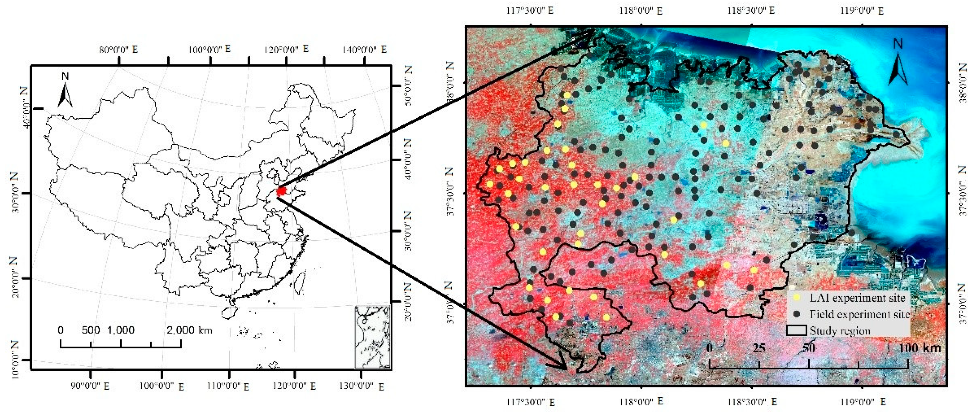
2.1. Study Area

The Yellow River Delta (YRD), a new alluvial land in Bohai Bay, is the transitional area formed from the land–sea interaction. The YRD region consists of Dongying city and Binzhou city, and covers an area of 15,564 km², approximately extending from 36.68° to 38.21° N latitude and 117.25° to 119.21° E longitude (Figure 1). This region has a typical warm and temperate monsoon climate, with sufficient light and heat. Clear seasonal variations in temperature, humidity and evaporation make it suitable for crop production. The YRD region has the most potential productivity in Shandong province and even China [68]. Coastal lowland with flat terrain is another characteristic of the study area. The elevation in the study region ranges from 1 to 20 m above sea level. With a short time of land formation and high ecological vulnerability, crop growth is largely restricted in many parts of YRD region, and the spatial heterogeneity of crop production is obvious [69,70,71].

Agriculture is the dominant industry in the YRD region, and the cropland area accounts for more than 65% of the region’s total area [11]. The main crop types are winter wheat, summer maize and cotton. Among them, winter wheat is the major grain in YRD region. The YRD region is a blended-planting region, consisting of double cropping and single cropping. Double cropping system is alternated by winter wheat and summer maize, which is commonly practiced [72]. Single cropping system is mainly planting cotton. There also very little spring wheat is cultivated. Due to soil salinization, it is hard to grow winter wheat in northeastern part of the region, where cotton is cultivated. Winter wheat is planted in late September to early October, and becomes mature in early to middle June of next year (Figure 2). The duration time for winter wheat is approximately 230–260 days [73]. Several phenological phases forms a complete growth cycle of winter wheat in one year, they are germination, seedling, tillering, overwintering, green-up, jointing, booting, heading, flowering, milk, the dough phase and maturity [11].

2.2. Data Collection

2.2.1. MODIS Data and Pre-Processing

The moderate resolution imaging spectroradiometer (MODIS) data was provided by the National Aeronautics and Space Administration’s Earth Observation System Clearing House Warehouse Inventory Search Tool (https://ladsweb.nascom.nasa.gov/search). The MOD09Q1 surface reflectance data from 2014 to 2015 were selected to extract winter wheat. The MOD09Q1 products were a re-project to Albers equal-area conic projection and resampled by the MODIS Reprojection Tool (MRT) (NASA, Washington, USA). Red and near-infrared reflectance were used to calculate the NDVI, which were provided at 250-m resolution from MOD09Q1 product every eight days. The NDVI was described using Equation (1):

$$NDVI=\frac{{\rho }_{NIR}-{\rho }_{RED}}{{\rho }_{NIR}+{\rho }_{RED}}$$

(1)

where ${\rho }_{NIR}$ and ${\rho }_{Red}$ are the visible red (620–670 nm) and near-infrared (841–876 nm) reflectance for the MODIS bands respectively.

The pixel quality was described by using quality assurance (QA) data of MOD09Q1. High quality corresponds to pixel values ranging from 0 to 3. Medium quality corresponds to pixel values ranging from 4 to 5. Low quality corresponds to pixel values ranging from 6 to 16. The corresponding weights were assigned to different quality levels. Weight values of 1, 0.5 and 0 were assigned to high quality, medium quality and low quality respectively.

Before winter wheat identification, smoothing algorithms should be used to reduce noise of time-series NDVI. The maximum value compositing (MVC) process can eliminate thick clouds, however, noise still exists which often generated by sensor parameter, solar altitude and aerosols. The Savitzky–Golay (SG) filter method was applied to reduce noises because of its simplicity and reliability. The SG filter achieves better denoising results than other mainstream algorithm in effectively reserving relative maximum, minimum and width [74]. The performance of the SG filter is exhibited in Figure 3. The SG filter smooths and computes derivatives of a set of consecutive values by executing simplified least squares-fit convolution [75]. For better performance of filtering, the data quality levels assigning with corresponding weights were used to identify spurious observations for the SG filter. Subsequently, the SG filter was applied by setting a window width of four, one envelope iterations, and an adaptation strength of two. Fitting iterations of SG filter were set to 2 instead of 1 in other similar study. However, the NDVI of double rice in rotation fallow period will be smoothed out at some double cropping field when the envelope iteration was set greater than 1. After several experiments and visual inspection, all the optimal fitting settings were set. The SG filter is described using Equation (2):

$$Y_j^{*}=\frac{{\sum }_{i=-m}^m{C}_i{Y}_{j+1}}{2m+1}$$

(2)

where Y denotes the original NDVI value, $Y_j^{*}$ is the filtered NDVI value, $C_i$ refers to the coefficient (smoothing window), $j$ is the running index of the original ordinate data table, and m is the half-width of the smoothing window [76].

2.2.2. Field Survey Data and Statistical Data

Two hundred and fifty pure pixels were manually selected from Google Earth. The pure pixels consisted of five vegetation types and each type had 50 pixels. The NDVI temporal profiles were constructed by using NDVI from September 2014 to June 2015. After averaging processing, and standard NDVI temporal profiles for each vegetation types were obtained.

One hundred and sixty-four field survey data were collected in March 2015 (Figure 1), and used to verify the accuracy of winter wheat classification. The filed site dataset had the same geographic coordinates, projected coordinates and location as MODIS data. A handheld GPS device Trimble GeoExplorer 3000 series (Trimble Navigation, Ltd, California, USA) was used to record geographical location and land use types. There were 84 samples of winter wheat, 33 samples of cotton, 18 samples of grassland, and 29 samples of woodland in the filed site dataset respectively. The results of classification and yield estimation were validated in two ways, verification with field sites and local agricultural statistics.

Ground-based LAI measurements from 2014 to 2015 aimed to collect data for calibration of LAI estimation models from the time series NDVI dataset. Thirty-six winter wheat plots were selected to measure LAI and its corresponding yield (Figure 1). We randomly divided the plots into two parts. Two-thirds of the plots were used for training, and one-third of the plots were used for testing. Regional LAI estimation model was established by using training plots, and the estimation result was validated by testing plots. To ensure the comparison of the extraction of representative mean LAI values with MODIS data at 250 m pixel resolution, the area for each plot is not less than 250 m × 250 m. Mean values of plots were used to represent the measured samples. Field location information was also recorded. The investigation times of LAI were the beginning of overwintering, green-up, jointing, heading and maturity, respectively. A LAI-2200 instrument (LI-COR Biotechnology, Ltd, Nebraska, USA) was used to collect LAI, and five measurements were done in each homogeneous area of MODIS pixel. LAI samples were randomly set and measured within each plot at a 45° angle between rows. A mean value of the five samples represented the plot value. To establish and verify the yield estimation model of winter wheat, the same thirty-six plots were selected to obtain the yields on 8 June 2015 during maturity stages. Five representative samples were selected within the scope of 250 m × 250 m. The mean value of each five samples within the scope represented the field value. An area of 1 m² in each wheat field was reaped and measured. The samples were taken back to the laboratory. After procedures of drying, weighing and threshing, the unit yield of winter wheat in each field was obtained. Two-thirds of the yield plots were used for training, and one-third of the plots were used for testing.

Meteorological data of nine meteorological stations covering the study area from 2014 to 2015 were provided by China Meteorological Data Service Center (http://data.cma.cn/). A daily meteorological dataset was selected, including air temperature, precipitation, sunshine duration, and radiation. Cumulative temperature of the green-up phase and the heading phase were calculated respectively by accumulating daily air temperature during the corresponding time period. A kriging method were used to interpolate meteorological data with a spatial resolution of 30 m. Cross-validation was performed and the validation results all met accuracy requirements.

The aridity index (AI) was defined as the ratio of annual potential evapotranspiration to precipitation. AI has been widely used to describe annual evaporation ratio in many studies. The AI dataset is provided by Data Center for Resources and Environmental Sciences, Chinese Academy of Sciences (RESDC) (http://www.resdc.cn). AI data was projected to an Albers equal area conic projection and extracted according to spatial extent of study area.

Soil properties such as soil salt content and soil organic matter content were determined from field soil samples which were collected in May 2015. A fishnet of 5 km × 5 km rectangular cells was created by ArcGIS 10.4 (ESRI, California, USA). Three hundred and forty-five soil samples at 0~20 cm plough layers were obtained with a soil drill. A kriging method was used to interpolate soil salt content and soil organic matter content with a spatial resolution of 30 m. Cross-validation was performed and the validation results all met accuracy requirements.

Digital Elevation Model (DEM) data was derived from Advanced Spaceborne Thermal Emission and Reflection Radiometer (ASTER) global digital elevation model (GDEM) Version 002 data with a spatial resolution of 30 m, which was provided by the Land Processes Distributed Active Archive Center (LP DAAC) of United States Geological Survey (USGS) (https://glovis.usgs.gov/). DEM data was projected to an Albers equal area conic projection and extracted to mask according to spatial extent of study area. On this basis, slope map was generated using Slope function of 3D Analyst tools in ArcGIS 10.4.

The spatial distribution of Yellow River was derived from the land-use map of the study area. The buffer analysis was done by distance function in ArcGIS 10.4. Distance to Yellow River was drawn by setting 1.0 km buffer radius.

Population data was from the sixth national census of China in 2010, which was collected at a community level. The Voronoi diagram was build and kriging interpolation was performed. Population density was obtained with a spatial resolution of 30 m.

The socio-economic status can be assessed by nighttime light data [77]. The visible infrared imaging radiometer suite (VIIRS) data was used, which was provided by the Earth Observation Group (EOG), National Geophysical Data Center (NGDC) at the National Oceanic and Atmospheric Administration (NOAA) (https://ngdc.noaa.gov/eog/download.html). The annual nighttime light image in 2015 was projected to an Albers equal area conic projection and extracted to study area with a spatial resolution of 500 m.

2.3. Methods

2.3.1. Winter Wheat Classification Based on Time-Series Similarity Measurement

In this study, there were two steps to performing the wheat discriminations. One was analysis of NDVI temporal profiles and the other was time-series similarity classification based on Minkowski distance.

NDVI Time Series Profiles Analysis

Each vegetation type had their unique temporal profiles behaviors, exhibiting their dynamic response to the environmental changes. Figure 4 exhibits the average temporal profiles for different vegetation types from September 2014 to June 2015 during the growing period of winter wheat. There were distinguishing features for woodland, grasslands, winter jujube, cotton and winter wheat in this period. As for winter wheat, the number of peaks had obvious characteristics.

The extracted NDVI temporal curves of winter wheat conformed to the typical phenological characteristics, which exhibited two consecutive periods of increase and decrease, with a maximum NDVI value of 0.8. The first peak appeared at the beginning of the overwintering, and the second peak existed in early May of the following year. Winter wheat could be separated from other vegetation based on the characteristic of NDVI temporal profile. Figure 4 exhibits the differences of time series NDVI profiles between winter wheat and other vegetation types.

Time-Series Similarity Measurement

A time-series similarity measurement basing on Minkowski distance was applied to discriminate winter wheat. The standard time series curves were obtained by selecting several pure pixels from each vegetation type. Figure 5 exhibits the principle of the Minkowski distance.

Suppose there are two groups of time series Q and S, whose lengths are $n$, namely $Q=\left\{q_1,q_2,\dots ,q_n\right\}$, $S=\left\{s_1,s_2,\dots ,s_n\right\}$, we need to calculate the path $P=\left\{p_1,p_2,\dots ,p_n\right\}$ between two groups of time series. $P$ is used to get the distance metric $Dmink\left(Q,S\right)$ which can be described by Equation (3):

$$Dmink={\left({{\displaystyle \sum }}_{t=1}^n\left|f_t^Q-f_t^S\right|\right)}^{\frac{1}{r}}$$

(3)

where $f_t^Q$ is the $f_Q\left(t\right)$ time series value at time $t$, $r$ is a user-defined integer, and $n$ is the images number available for the yearly rice cropping system classification. In our study, $r$ was set to 2. When the parameter $r$ was set to 2, the Minkowski distance can be regarded as the Euclidean distance. Due to its nonlinear character, Euclidean distance is more sensitive to outlier values and useful to distinguish other objects. The Minkowski distances between standard time series curves and curves to be processed were measured by a programming technique in MATLAB (2017a) (MathWorks, Natick, MA, USA).

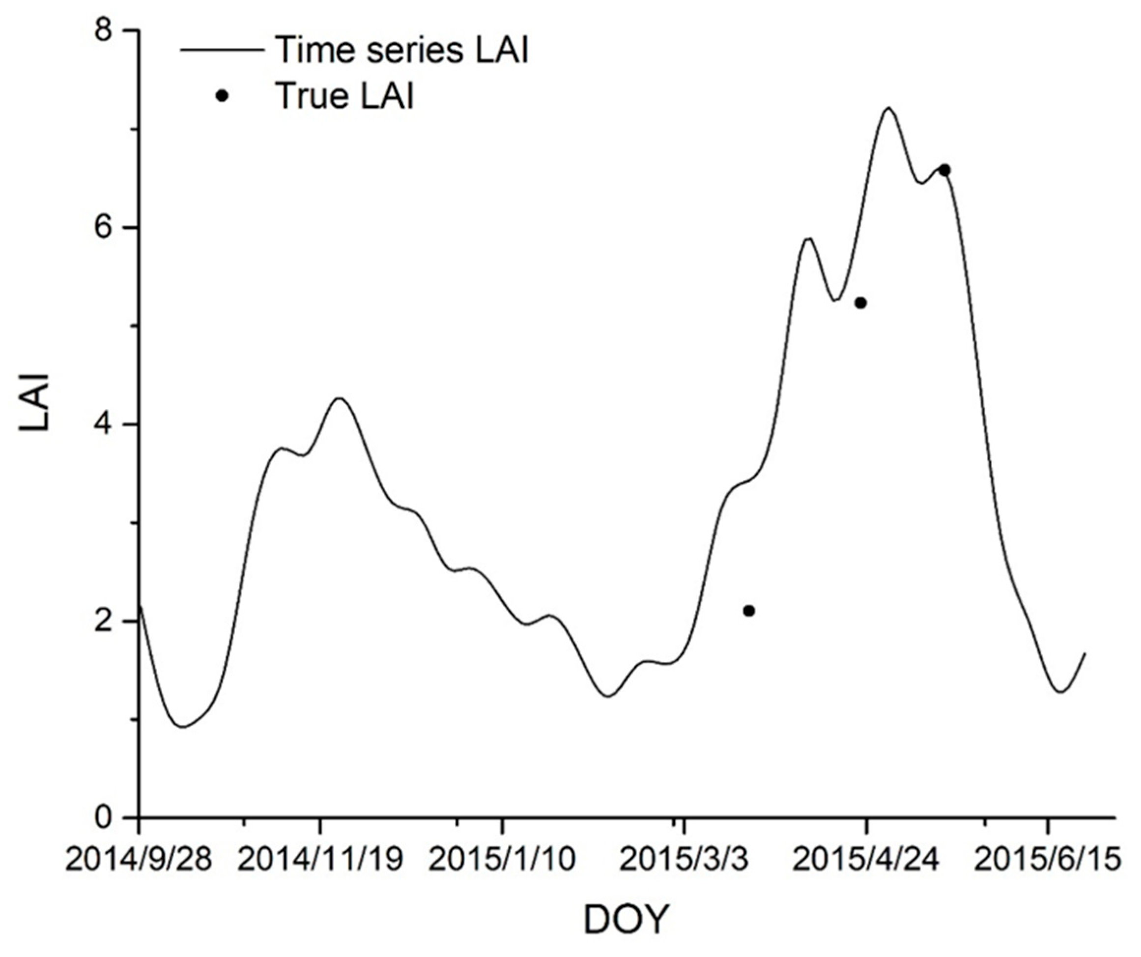
2.3.2. Time Series LAI Estimation

Ground-measured LAI and its corresponding NDVI were used to establish statistical model of different growth period. The retrieval effect of LAI differed in each growth period. The simulation results of three models (unitary linear model, quadratic polynomial model and exponential model) were analyzed. The modelling results indicated that the correlation coefficients between NDVI and LAI in vegetative growth period were higher than that in whole growing period. The correlation coefficients in reproductive growth period were not significant. LAI inversion during vegetative growth period was modelled. The estimation accuracy was evaluated by R² and root mean square error (RMSE). Figure 6 shows the regression results of NDVI and ground-measured LAI. The regression function was described by Equation (4):

$$y=9.5689x-1.3077$$

(4)

The regression model exhibited a high degree of fitting to the equation and small estimation error. R² and RMSE were 0.7536 and 0.21 respectively. According to the best-fitting model of LAI, the simulated LAI at eight-day intervals were obtained.

The LAI curve exhibited in Figure 7 indicates the growth cycle of winter wheat, where the LAI value lined up, and the abscissa describes time. The LAI time series curves of winter wheat were obtained, reflecting the LAI dynamic changes in the growing period. Features of time series curves agreed with reality, showing the information of wheat growth. The LAI retrieval accuracy of winter wheat is relatively high which could meet the needs of yield estimation for winter wheat.

2.3.3. Yield Modeling Based on LAI Phenological Features

To verify the validity of phenological information in yield estimation of winter wheat, the yield estimation model based on phenological features of LAI was established. Inspired by Chul et al. [11], seven important phenological metrics were chosen for their closely relation with yields, including LAI in green-up phase, maximum LAI in whole growing period, accumulated LAI from green-up phase to maturity phase, average LAI in whole growing period, standard deviation of LAI in whole growing period, changing rate of LAI in vegetative growth period, and changing rate of LAI in reproductive growth period.

LAI in green-up phase represents the LAI value at the beginning of vigorous growth for winter wheat. The regional LAI in average green-up date represents the LAI in green-up phase. Maximum LAI, by definition, is the maximum value of LAI generally occurs during the period from heading to flowering, representing the formation of nutrient organs and the transporting ability from substance to wheat grains. The LAI in average heading date could represent the maximum LAI in whole growing period. Accumulated LAI from green-up phase to maturity phase represents the overall status of vegetation. Average LAI in whole growing period represents the constant vegetation status. The standard deviation of LAI in whole growing period is defined as the change of the average LAI value in whole growth period.

The changing rate of LAI in vegetative growth period refers to the growing speed or frequency from green-up phase to heading phase. The number of spikes and grains are finally determined in the vegetative growth period which period is a critical period. The changing rate of LAI in vegetative growth period can be described by Equation (5):

$$RCvg=\left|\frac{{\sum }_{x=1}^{\overline{N}}{f}^{\prime }\left(x,a\right)}{{\mathrm{Day}}_{max}-{\mathrm{Day}}_{rev}}\right|$$

(5)

where $RCvg$ is the changing rate of LAI in vegetative growth period, $f\left(x, a\right)$ is the polynomial function for LAI time-series profile, ${\mathrm{Day}}_{max}$ denotes the day of year when LAI value reaches the maximum (usually in heading date), ${\mathrm{Day}}_{rev}$ denotes the day of year when winter wheat enters into green-up date, and N is the number of images (also the difference between ${\mathrm{Day}}_{max}$ and ${\mathrm{Day}}_{\mathrm{rev}}$) during vegetative growth period.

Changing rate of LAI in reproductive growth period, by definition, is the growing speed or frequency from heading phase to maturity phase. The reproductive growth period is the key period for determining grain quality and forming final yield. The changing rate of LAI in reproductive growth period can be described by Equation (6):

$$RCrg=\left|\frac{{\sum }_{x=1}^{\overline{N}}{f}^{\prime }\left(x,a\right)}{{\mathrm{Day}}_{mat}-{\mathrm{Day}}_{max}}\right|$$

(6)

where $RCrg$ is the changing rate of LAI in reproductive growth period, $f\left(x,a\right)$ is the polynomial function for LAI time-series profile, ${\mathrm{Day}}_{max}$ denotes the day of year when LAI value reaches the maximum (usually in heading date), ${\mathrm{Day}}_{mat}$ denotes the day of year when winter wheat enters into harvest time, and N is the number of images (also the difference between ${\mathrm{Day}}_{max}$ and ${\mathrm{Day}}_{mat}$) during reproductive growth period.

The most efficient parameters were selected as elements to construct the ultimate yield estimation model through the stepwise multi-elemental regression method. Regional yield of winter wheat was obtained and the estimation accuracy was then validated. The multi-element linear regression equation can be described by Equation (7):

$$\begin{array}{cc}y=1023.91& +{\mathrm{LAI}}_{max}\times 140.04+LA{I}_{stnd}\times 294.21+{\mathrm{LAI}}_{greenup}\times 54.26\\ & \hspace{1em}-LA{I}_{sum}\times 11.68-R{C}_{vg}\times 559.79-R{C}_{rg}\times 993.09\end{array}$$

(7)

where $y$ denotes the yield, ${\mathrm{LAI}}_{max}$ refers to maximum LAI in whole growing period, ${\mathrm{LAI}}_{stnd}$ is standard deviation of LAI in whole growing period, ${\mathrm{LAI}}_{greenup}$ is LAI in green-up phase, ${\mathrm{LAI}}_{sum}$ is accumulated LAI from green-up phase to maturity phase, $RCrg$ is the changing rate of LAI in vegetative growth period, and $RCrg$ is the changing rate of LAI in reproductive growth period. Note that the phenological feature of average LAI was excluded in the model building due to relatively low estimation accuracy.

2.3.4. Geographical Detector

Spatial heterogeneity is one of the basic characteristics of geographical phenomena. The geographical detector is developed to detect spatial heterogeneity [59]. This method overcomes limitations of traditional mathematical statistical models, such as many assumptions and large data requirements. Both numerical data and qualitative data can be detected in geodetector method. There are four functions in geodetector, including risk detector, factor detector, ecological detector and interaction detector.

Factor detector measures spatial stratified heterogeneity of dependent variable Y, and determinant power of independent variables X on the spatial heterogeneity of Y both linearly and nonlinearly [78], which can be accomplished by q-statistic and described by Equation (8):

$$\begin{gathered} q=1-\frac{{\sum }_{h=1}^L{N}_h{\sigma }_h^2}{N{\sigma }^2}=1-\frac{SSW}{SST} \\ SSW={\displaystyle \sum }_{h=1}^L{N}_h{\sigma }_h^2, SST=N{\sigma }^2 \end{gathered}$$

(8)

where $q$ indicates the explanatory power of variable X on event Y. $h=1,\dots ,L$ is the strata (classification) of the explanatory variable X, $N_h$ and $N$ stand for the number of units in strata $h$ and the whole region, respectively. ${\sigma }_h^2$ and ${\sigma }^2$ refer to the variance of Y in strata $h$ and the whole region. $SSW$ and $SST$ represent within sum of squares and total sum of squares. The value of $q$ ranges from 0 to 1. There is no association between Y and X when $q$ value equals to 0. Factor X completely controls Y when $q$ value equals to 1. The larger the $q$ value, the stronger the explanatory power of X on Y, and vice versa. Note that X should be a categorical variable, and the number of strata $L$ might range from 2 to 10. Stratification should be done when X is numerical.

Interaction detector identifies interaction between two influencing factors, which detects whether the factors will increase or decrease the explanatory power of Y, or the factors on Y are independent of each other. The $q$ values of $X1$, $X2$ and their interactions ($X1\cap X2$) are calculated. $q\left(X1\cap X2\right)$, $q\left(X1\right)$ and $q\left(X2\right)$ then are compared. There are five types of interaction between two covariates. The interaction of factors would weaken nonlinearly when $q\left(X1\cap X2\right)<\mathrm{Min}\left(q\left(X1\right),q\left(X2\right)\right)$. The uni-factor would weaken nonlinearly when $\mathrm{Min}\left(q\left(X1\right),q\left(X2\right)\right)<q\left(X1\cap X2\right)<\mathrm{Max}\left(q\left(X1\right),q\left(X2\right)\right)$. The interaction of bi-factor would enhance when $q\left(X1\cap X2\right)>\mathrm{Max}\left(q\left(X1\right),q\left(X2\right)\right)$. The factors are independent when $q\left(X1\cap X2\right)=q\left(X1\right)+q\left(X2\right).$ The interaction of factors would enhance nonlinearly when $q\left(X1\cap X2\right)>q\left(X1\right)+q\left(X2\right)$.

Factor detector and interaction detector was used to examine the dominant factors and interactions influencing spatial heterogeneity of winter wheat yield in YRD region. Thirteen factors involving natural and human factors were selected, covering cumulative temperature for green-up phase ($X1$), cumulative temperature for heading phase ($X2$), precipitation ($X3$), sunshine duration ($X4$), radiation ($X5$), aridity index ($X6$), soil salinity ($X7$), organic matter ($X8$), DEM ($X9$), slope ($X10$), distance to Yellow River ($X11$), population density ($X12$) and nighttime light ($X13$).

A fishnet of 250 m × 250 m rectangular cells was created by ArcGIS 10.4. Density of grid points was determined according to actual spatial pattern of winter wheat. To investigate relationships between influencing factors and winter wheat yield, 1456 sampling points were selected. Each factor was stratified by natural breakpoint method with seven grades in each category. The yields and corresponding stratification values of each factor were extracted to points, and then calculation was performed by the geo-detector tool.

3. Results

3.1. Spatial Pattern of Winter Wheat

The spatial distribution of winter wheat was mapped by calculating Minkowski distance based on time-series similarity analysis. The threshold of calculation was set as 2.64 to extract winter wheat. Figure 8 exhibits the spatial pattern of winter wheat. Generally, winter wheat was mainly distributed in the southwest of the study region, and a small amount of winter wheat was found along the rivers in the northeastern part of the study region.

The classification accuracy was validated with field dataset and agricultural statistical data respectively. The percentage of pixels correctly classified was defined as the overall classification accuracy. Together with the kappa coefficient, the classification results were validated with ground data.

Table 1. The confusion matrix for winter wheat identification.

Vegetation Type	Winter Wheat	Cotton	Woodland	Grassland
Numbers of samples	84	33	29	18
Numbers of samples classified as winter wheat	74	0	3	7
Total accuracy	88.09%

indicates the confusion matrix for winter wheat classification, showing a good agreement with the pixel-by-pixel comparisons. The overall accuracy was 88.09% and the Kappa coefficient was 0.81. There were 74 sampling points were classified correctly as winter wheat among the 84 sampling points. There were 10 points were misclassified as winter wheat among the 80 non-winter wheat crop field points.

Due to the high similarity between grassland and winter wheat in time-series profiles, some grasslands were misclassified into winter wheat. The separability of winter wheat from the grassland should consider the similarity characteristics of time series profile in future studies. The mixed pixel problems can be clearly noticed in northeastern part of study region, where winter wheat was grown in small areas with sufficient water near the riverbank. Compared to the spatial resolution of MODIS (6.25 ha), the area of winter wheat fields in this area is quite small (usually less than 1 hectare). Therefore, such a small area cannot be detected by MODIS.

The classification results were also validated with agricultural statistics in 2015 provided by the municipal government. The acreage accuracy of winter wheat was 89.75% at the municipal level, verifying the ability of proposed method in winter wheat identification.

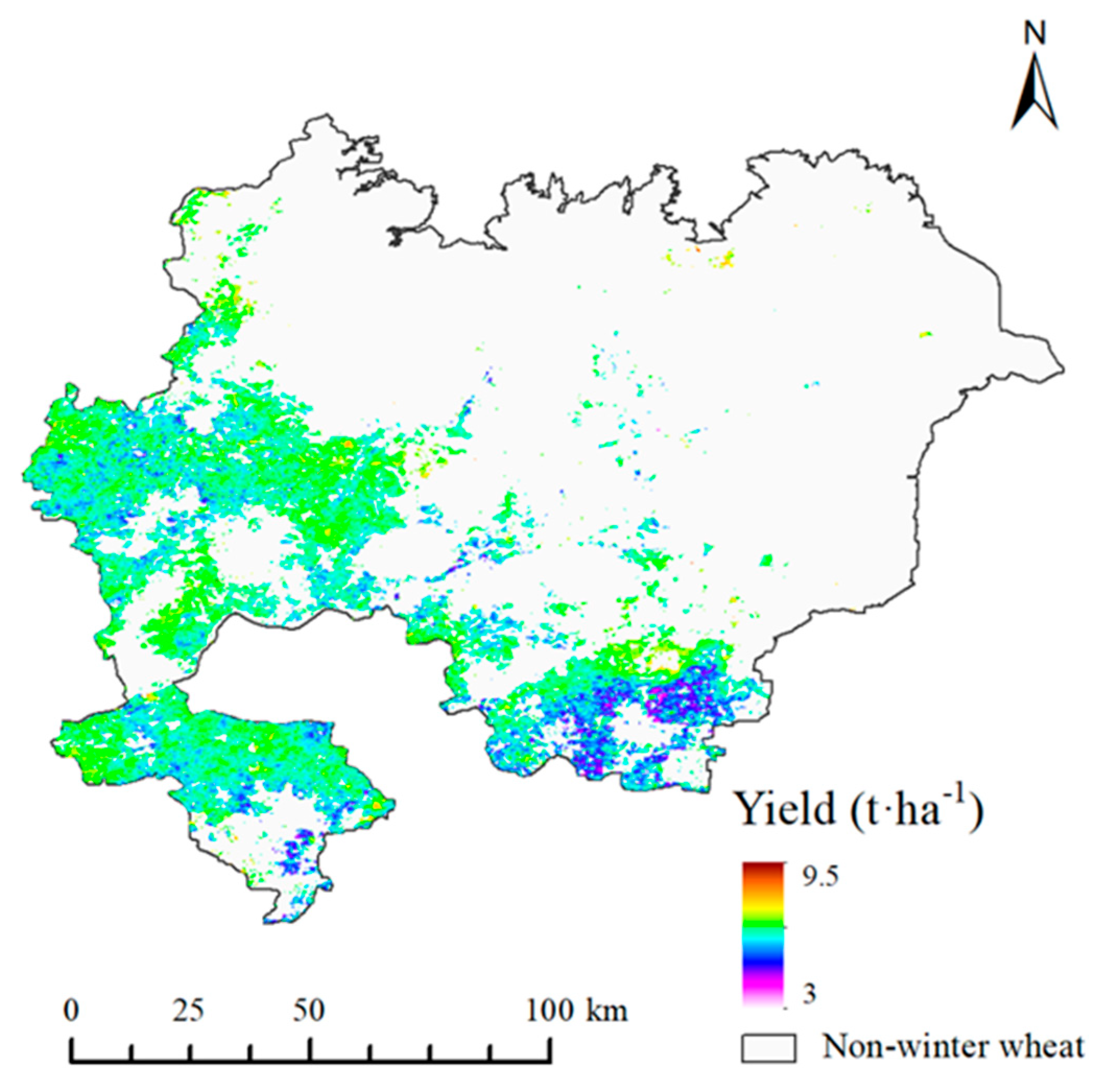
3.2. Winter Wheat Yield Estimation Based on Phenological Features

The regional distribution of winter wheat yield was obtained by integrating each LAI phenological features in multi-element linear regression model. To avoid overfitting, the Leave One Out Cross Validation (LOOCV) method of cross-validation was used to validate the established yield estimation. There was a good correlation between measured yield and estimated yield, exhibiting a R² value of 0.74 at significant level (P < 0.01), and a RMSE of 1.02 t ha⁻¹. Note that when the actual yield was relatively small (less than 8 t ha⁻¹), the estimated yield turned to be larger than field measured records. When the actual planting area was large, the estimated yield turned to be smaller (Figure 9).

The spatial pattern of winter wheat yield showed a significant heterogeneity from south to north (Figure 10). Winter wheat yield exhibited a decreasing trend south to north, which conformed to the actual distribution of winter wheat yield in YRD region. The average yield per unit area of winter wheat was 6.9 t ha⁻¹ and the standard deviation was 0.76 t ha⁻¹, which is generally consist with local actual yields, providing a simpler and reliable way to estimate yield based on time series phenological features.

3.3. Analysis of Determinants for Spatial Heterogeneity of Winter Wheat Yield

To investigate which factors was most closely related to spatial heterogeneity of winter wheat yield in YRD region, the relationships between thirteen factors and winter wheat yield were analyzed, and the q value of each influencing factor on winter wheat yield was calculated. The factor detector results indicated that there was a significant difference in explanatory power of influencing factors on spatial heterogeneity of winter wheat yield (

Table 2. The q values of influencing factors in Yellow River Delta (YRD) region.

Influencing Factor	q Value
Cumulative temperature for heading phase	0.49
Soil salinity	0.36
Cumulative temperature for green-up phase	0.32
Precipitation	0.27
Population density	0.27
Sunshine duration	0.23
Aridity index	0.23
Organic matter	0.22
Distance to Yellow River	0.22
Radiation	0.07
DEM	0.06
Slope	0.03
Nighttime light	0.02

). The corresponding q value of each influencing factor, ranging from highest to lowest, were cumulative temperature for heading phase ($X2$), soil salinity ($X7$), cumulative temperature for green-up phase ($X1$), precipitation ($X3$), population density ($X12$), sunshine duration ($X4$), aridity index ($X6$), organic matter ($X8$), distance to Yellow River ($X11$), radiation ($X5$), DEM ($X9$), slope ($X10$) and nighttime light ($X13$).

Cumulative temperature for heading phase, soil salinity and cumulative temperature for green-up phase were three dominant determinants, which explanatory powers account for 0.49, 0.46 and 0.32 respectively. Precipitation, population density, sunshine duration, aridity index, organic matter and distance to Yellow River were secondary determinants, which explanatory powers were above 0.2. Winter wheat yield was less affected by radiation, DEM, slope and nighttime light, with explanatory power of less than 0.1.

An interaction detector was used to investigate the interactions between any two influencing factors. The interaction module results indicated that the explanatory power of any two-factor interaction on wheat yield was greater than that of a single factor, indicating that the spatial heterogeneity of winter wheat yield was largely affected by interactions between factors. The explanatory power of the interactions was sorted according to statistical results, where q value were greater than 0.4.

Table 3. The dominant interactions between two influencing factors.

Interaction Type	q Value
Cumulative temperature for green-up phase ∩ soil salinity	0.69
Cumulative temperature for heading phase ∩ soil salinity	0.64
Cumulative temperature for green-up phase ∩ aridity index	0.60
Cumulative temperature for green-up phase ∩ distance to Yellow River	0.59
Cumulative temperature for heading phase ∩ nighttime light	0.52
Cumulative temperature for heading phase ∩ distance to Yellow River	0.51
Soil salinity ∩ precipitation	0.50
Soil salinity ∩ organic matter	0.49
Soil salinity ∩ aridity index	0.45
Soil salinity ∩ population density	0.45
Soil salinity ∩ nighttime light	0.43
Soil salinity ∩ sunshine duration	0.42
Soil salinity ∩ radiation	0.42
Soil salinity ∩ slope	0.41
Soil salinity ∩ DEM	0.40

exhibited dominant interactions with corresponding q values. The enhancement between cumulative temperature for the green-up phase and soil salinity, cumulative temperature for the heading phase and soil salinity, and cumulative temperature for green-up phase and aridity index were the most significant interactions, and the q values of the interactions were higher than single factor.

The interaction between cumulative temperature for the green-up phase and soil salinity was the most dominant controlling factor for spatial heterogeneity of winter wheat yield, which has highest explanatory power, with a q value of 0.69. The winter wheat yield would vary obviously under conditions of different soil salinity and similar cumulative temperature for the green-up phase, or different cumulative temperature for green-up phase and similar soil salinity. For example, the winter wheat yield with soil salt content of 0.05% was significantly different from that of 0.49% when the cumulative temperature for green-up phase was 155 degree days, and the winter wheat yield with cumulative temperature for green-up phase of 125 degree days obviously differed from that of 158 degree days when the soil salt content was 0.05%. The second dominant controlling factor was the interaction between cumulative temperature for the heading phase and soil salinity with a q value of 0.64. The third dominant controlling factor was cumulative temperature for green-up phase and aridity index, which had a q value of 0.60. The interactions ranking from first to sixth all were combinations of cumulative temperature and other factors. In addition, the combination of soil salinity and other factors greatly increased the explanatory power of a single factor on wheat yield, which showed nonlinear enhancement.

4. Discussion

According to the results of Section 3.1, we found that the spatial pattern of winter wheat is consistent with previous studies, indicating a decreasing trend according to the distance to the sea [11]. Figure 10 exhibits the distribution shift for winter wheat, indicating the ability of remote sensing to capture the spatial heterogeneity in the YRD region. However, mixed pixels in remote sensing data led to the uncertainties of identifying winter wheat. When identifying winter wheat and estimating its yield, precise spatial information is required. Indeed, for monitoring crop growth and estimating crop area by remote sensing over a Chinese site, spatial resolution of 120 m and 30 m are often needed respectively [79]. Time-series MODIS has been widely used to monitor crop condition where the field areas are much larger than the 250 m pixel size, allowing for individual crops classification [49,80]. However, the results of classification accuracy for winter wheat would be affected by the spatial resolution of 250 m. We should note that the extraction accuracy was not satisfying in northeastern areas of study region. There was a small amount of winter wheat scattering along the rivers where winter wheat was cultivated on a small scale (usually less than 1 ha). The mixed pixel caused by small-scale cultivation would affect classification accuracy. Besides the requirement of spatial information, the temporal information was also of great importance in crop yield estimation. The 8-d time-series used in our study had more accurate temporal resolution than other remote sensing sources, however, these cannot fully reflect the phenological characteristics for winter wheat. In addition, the usage of DPC (the day of pixel composite) information would significantly improve accuracy of agricultural monitoring. However, DPC information is not contained in the MOD09Q1 product, which also may impact the results accuracy. The Sentinel-2 satellite with 10 m spatial resolution and 5-d temporal resolution will be a good solution for mixed pixel at regional scale in our future research, which satellite launched in June, 2015.

According to the results of geodetector, cumulative temperature and soil salinity were key determinants greatly affecting winter wheat yield. Many scholars showed evidences of the two factors on crop yields [81,82,83,84,85,86], which are consistent with our results. Since the complexity of winter wheat growth processes, an influencing factor often did not work independently but interacted together. The results from interaction module of geodetector indicate that the explanatory power of interaction of cumulative temperature for green-up phase and soil salinity was over 69%. Chu et al. [73] found that cumulative temperature and soil salinity significantly influenced phenology of winter wheat. The delay of the green-up phase and the advance of the heading phase will shorten the time for vegetative growth of winter wheat, and ultimately affected the winter wheat yield with the increase of soil salt content. This finding showed good agreement with our study, which indicated that the interaction of cumulative temperature and soil salinity largely affects the spatial heterogeneity of winter wheat yield. Hence, several measures are recommended to effectively increase and stabilize wheat yields in the YRD region, including improving irrigation and drainage systems to reduce soil salinity [87,88], selecting salt-tolerant winter wheat varieties [89,90], and improving agronomy techniques to extend effective cumulative temperature, such as mulching and reasonable arrangements for sowing [91].

The process of crop growth and its ultimate yield is complex, and seasonal soil salinity dynamics lacked consideration in our study. In YRD region, the soil salinity is highly related with groundwater dynamics and has obvious seasonal fluctuations [92]. It is characterized by soil salinity accumulation in spring, desalination in summer, pick-up in autumn, and latent salinity in winter. In the seasonal variation during a year, the salt deposition period is consistent with the growth period of winter wheat, which seriously affects the growth and yield of winter wheat. In addition, soil salinity significantly affects wheat growth throughout the growing period [85]. An interesting problem we hope to address in the near future is identifying phenological periods in which soil salinity has the greatest impact on wheat yield under the condition of constant cumulative temperature.

5. Conclusions

The current study explored spatial heterogeneity of winter wheat yield and its determining factors in the YRD region by using a yield estimation model integrated with phenological information and the geographical detector method. Applying these methodologies, several conclusions were gained. Winter wheat was mapped through the time-series similarity measurement basing on Minkowski distance with a relatively high accuracy, exhibiting a concentrated distribution in the southwest of the study area. Winter wheat yield was estimated by combining phenological information into the yield estimation model, showing a decreasing trend from south to north. Cumulative temperature, soil salinity and the interaction between cumulative temperature and soil salinity were three key determinants for spatial heterogeneity of winter wheat yield. According to the above results, several measures should be taken to increase winter wheat yield, such as improving irrigation and drainage systems to reduce soil salinity, planting salt-tolerant winter wheat varieties, mulching and reasonable arrangements for sowing. The findings offer the potential to explore spatial heterogeneity of winter wheat yield and its determinants, and provide scientific basis for improving regional wheat yield, as well as effective decision-making support to local government for agricultural planning and management, ensuring food security and promoting the sustainable agricultural development.

References

1. Macdonald, R.B.; Hall, F.G. Global Crop Forecasting. Science 1980, 208, 670–679. [Google Scholar] [CrossRef] [PubMed]
2. Christiansen, F. Food Security, Urbanization and Social Stability in China. J. Agrar. Change. 2009, 9, 548–575. [Google Scholar] [CrossRef]
3. Abraham, B.; Araya, H.; Berhe, T.; Edwards, S.; Gujia, B.; Khadka, R. The system of crop intensification: Reports from the field on improving agricultural production, food security, and resilience to climate change for multiple crops. Agric. Food Secur. 2014, 3, 4. [Google Scholar] [CrossRef] [Green Version]
4. Cao, M.; Zhu, Y.H.; Lü, G.N.; Chen, M.; Qiao, W.F. Spatial distribution of global cultivated land and its variation between 2000 and 2010, from both agro-ecological and geopolitical perspectives. Sustainability 2019, 11, 1242. [Google Scholar] [CrossRef] [Green Version]
5. Dong, J.; Xiao, X. Evolution of regional to global paddy rice mapping methods: A review. Isprs J. Photogramm. Remote Sens. 2016, 119, 214–227. [Google Scholar] [CrossRef] [Green Version]
6. Rowan, J.N.; Downes, R.G. A Study of the Land in North-Western Victoria: T.C. 2; Soil Conservation Authority: Victoria, Australia, 1963. [Google Scholar]
7. Fraisse, C.W.; Sudduth, K.A.; Kitchen, N.R. Delineation of site-specific management zones by unsupervised classification of topographic attributes and soil electrical conductivity. Trans. Am. Soc. Agric. Eng. 2001, 44, 155–166. [Google Scholar] [CrossRef] [Green Version]
8. Kasper, T.C.; Pulido, D.J.; Fenton, T.E.; Colvin, T.S.; Karlen, D.L.; Jaynes, D.B.; Meek, D.W. Relationship of corn and soybean yield to soil and terrain properties. J. Agron. 2004, 96, 700–709. [Google Scholar] [CrossRef] [Green Version]
9. Cox, M.S.; Gerard, P.D.; Wardlaw, M.C.; Abshire, M.J. Variability of selected soil properties and their relationships with soybean yield. Soil Sci. Soc. Am. J. 2003, 67, 1296–1302. [Google Scholar] [CrossRef]
10. Jung, W.K.; Kitchen, N.R.; Sudduth, K.A.; Kremer, R.J.; Motavilli, P.P. Relationship of apparent soil electrical conductivity to claypan soil properties. Soil Sci. Soc. Am. J. 2005, 69, 883–892. [Google Scholar] [CrossRef] [Green Version]
11. Lin, C.H.U.; Liu, Q.S.; Huang, C.; Liu, G.H. Monitoring of winter wheat distribution and phenological phases based on MODIS time-series: A case study in the Yellow River Delta, China. J. Integr. Agric. 2016, 15, 2403–2416. [Google Scholar]
12. Kastens, J.H. Image masking for crop yield forecasting using AVHRR NDVI time series imagery. Remote Sens. Environ. 2005, 99, 341–365. [Google Scholar] [CrossRef]
13. Tennakoon, S.B.; Murty, V.V.N.; Eiumnoh, A. Estimation of cropped area and grain yield of rice using remote sensing data. Int. J. Remote Sens. 1992, 13, 427–439. [Google Scholar] [CrossRef]
14. Fritz, S.; Massart, M.; Savin, I.; Gallego, J.; Rembold, F. The use of MODIS data to derive acreage estimations for larger fields, A case study in the south-western Rostov region of Russia. Int. J. Appl. Earth Obs. Geoinf. 2008, 10, 453–466. [Google Scholar] [CrossRef]
15. Li, Q.; Wu, B.; Jia, K.; Dong, Q.; Eerens, H.; Zhang, M. Maize acreage estimation using ENVISAT MERIS and CBERS-02B CCD data in the North China Plain. Comput. Electron. Agric. 2011, 78, 208–214. [Google Scholar] [CrossRef]
16. Wu, B.; Li, Q. Crop planting and type proportion method for crop acreage estimation of complex agricultural landscapes. Int. J. Appl. Earth Obs. Geoinf. 2012, 16, 101–112. [Google Scholar] [CrossRef]
17. Huete, A.; Didan, K.; Miura, T.; Rodriguez, E.P.; Gao, X.; Ferreira, L.G. Overview of the radiometric and biophysical performance of the MODIS vegetation indices. Remote Sens. Environ. 2002, 83, 195–213. [Google Scholar] [CrossRef]
18. Potgieter, A.B.; Apan, A.; Hammer, G.; Dunn, P. Estimating winter crop area across seasons and regions using time-sequential MODIS imagery. Int. J. Remote Sens. 2011, 32, 4281–4310. [Google Scholar] [CrossRef]
19. Wardlow, B.D.; Egbert, S.L.; Kastens, J.H. Analysis of time-series MODIS 250 m vegetation index data for crop classification in the US Central Great Plains. Remote Sens. Environ. 2007, 108, 290–310. [Google Scholar] [CrossRef] [Green Version]
20. Mingwei, Z.; Qingbo, Z.; Zhong, Z.; Xin, C.; Jia, L.; Yong, Z.; Chongfa, C. Crop discrimination in Northern China with double cropping systems using Fourier analysis of time-series MODIS data. Int. J. Appl. Earth Obs. Geoinf. 2008, 10, 476–485. [Google Scholar] [CrossRef]
21. Setiyono, T.D.; Quicho, E.D.; Gatti, L.; Campos-Taberner, M.; Busetto, L.; Collivignarelli, F.; Garcia-Haro, F.J.; Boschetti, M.; Khan, N.I.; Holecz, F. Spatial rice yield estimation based on MODIS and Sentinel-1 SAR Data and ORYZA crop growth model. Remote Sens. 2018, 10, 293. [Google Scholar] [CrossRef] [Green Version]
22. Liaqat, M.U.; Cheema, M.J.M.; Huang, W.; Mahmood, T.; Zaman, M.; Khan, M.M. Evaluation of MODIS and Landsat multiband vegetation indices used for wheat yield estimation in irrigated Indus Basin. Comput. Electron. Agric. 2017, 138, 39–47. [Google Scholar] [CrossRef]
23. He, M.; Kimball, J.S.; Maneta, M.P.; Maxwell, B.D.; Moreno, A. Regional crop gross primary production and yield estimation using fused Landsat-MODIS data. Remote Sens. 2018, 10, 372. [Google Scholar] [CrossRef] [Green Version]
24. Galford, G.L.; Mustard, J.F.; Melillo, J.; Gendrin, A.; Cerri, C.C.; Cerri, C.E. Wavelet analysis of MODIS time series to detect expansion and intensification of row-crop agriculture in Brazil. Remote Sens. Environ. 2008, 112, 576–587. [Google Scholar] [CrossRef]
25. Townshend, J.R.; Justice, C.O.; Kalb, V. Characterization and classification of South American land cover types using satellite data. Int. J. Remote Sens. 1987, 8, 1189–1207. [Google Scholar] [CrossRef]
26. Eastman, J.R. Long sequence time series evaluation using standardized principal components. Photogramm. Eng. Remote Sens. 1993, 59, 991–996. [Google Scholar]
27. Brown, J.F.; Loveland, T.R.; Merchant, J.W.; Reed, B.C.; Ohlen, D.O. Using multisource data in global land-cover characterization: Concepts, requirements, and methods. Photogramm. Eng. Remote Sens. 1993, 59, 977–987. [Google Scholar]
28. Wardlow, B.D.; Egbert, S.L. Large-area crop mapping using time-series MODIS 250 m NDVI data: An assessment for the US Central Great Plains. Remote Sens. Environ. 2008, 112, 1096–1116. [Google Scholar] [CrossRef]
29. Geerken, R.; Zaitchik, B.; Evans, J.P. Classifying rangeland vegetation type and coverage from NDVI time series using Fourier Filtered Cycle Similarity. Int. J. Remote Sens. 2005, 26, 5535–5554. [Google Scholar] [CrossRef]
30. Niennattrakul, V.; Srisai, D.; Ratanamahatana, C.A. Shape-based template matching for time series data. Knowl. Based Syst. 2011, 26, 1–8. [Google Scholar] [CrossRef]
31. Lloyd, D. A phenological classification of terrestrial vegetation cover using shortwave vegetation index imagery. Remote Sens. 1990, 11, 2269–2279. [Google Scholar] [CrossRef]
32. Reed, B.C.; Brown, J.F.; VanderZee, D.; Loveland, T.R.; Merchant, J.W.; Ohlen, D.O. Measuring phenological variability from satellite imagery. J. Veg. Sci. 1994, 5, 703–714. [Google Scholar] [CrossRef]
33. Zhong, L.; Hawkins, T.; Biging, G.; Gong, P. A phenology-based approach to map crop types in the San Joaquin Valley, California. Int. J. Remote Sens. 2011, 32, 7777–7804. [Google Scholar] [CrossRef]
34. Dong, J.; Xiao, X.; Kou, W.; Qin, Y.; Zhang, G.; Li, L.; Jin, C.; Zhou, Y.; Wang, J.; Biradar, C.; et al. Tracking the dynamics of paddy rice planting area in 1986–2010 through time series Landsat images and phenology-based algorithms. Remote Sens. Environ. 2015, 160, 99–113. [Google Scholar] [CrossRef]
35. Lhermitte, S.; Verbesselt, J.; Verstraeten, W.W.; Coppin, P. A comparison of time series similarity measures for classification and change detection of ecosystem dynamics. Remote Sens. Environ. 2011, 115, 3129–3152. [Google Scholar] [CrossRef]
36. Wang, X.; Mueen, A.; Ding, H.; Trajcevski, G.; Scheuermann, P.; Keogh, E. Experimental comparison of representation methods and distance measures for time series data. Data Min. Knowl. Discov. 2013, 26, 275–309. [Google Scholar] [CrossRef] [Green Version]
37. Zhang, G.H.B.; Kinsner, W. Electrocardiogram data mining based on frame classification by dynamic time warping matching. Comput. Methods Biomech. Biomed. Eng. 2009, 12, 701–707. [Google Scholar] [CrossRef]
38. Potgieter, A.B.; Apan, A.; Dunn, P.; Hammer, G. Estimating crop area using seasonal time series of Enhanced Vegetation Index from MODIS satellite imagery. Crop. Pasture Sci. 2007, 58, 316–325. [Google Scholar] [CrossRef] [Green Version]
39. Hao, P.; Niu, Z.; Wang, L.; Abulikmu, A.; Wang, X. Planting Information Extraction of Cotton based on MODIS EVI Time-series Matching: A Case Study of Bole County in Xinjiang. Remote Sens. Technol. Appl. 2013, 28, 77. [Google Scholar]
40. Hamar, D.; Ferencz, C.; Lichtenberger, J.; Tarcsai, G.; Ferencz-Arkos, I. Yield estimation for corn and wheat in the Hungarian Great Plain using Landsat MSS data. Int. J. Remote Sens. 1996, 17, 1689–1699. [Google Scholar] [CrossRef]
41. Doraiswamy, P.C.; Hatfield, J.L.; Jackson, T.J.; Akhmedov, B.; Prueger, J.; Stern, A. Crop condition and yield simulations using Landsat and MODIS. Remote Sens. Environ. 2004, 92, 548–559. [Google Scholar] [CrossRef]
42. Benedetti, R.; Rossini, P. On the use of NDVI profiles as a tool for agricultural statistics: The case study of wheat yield estimate and forecast in Emilia Romagna. Remote Sens. Environ. 1993, 45, 311–326. [Google Scholar] [CrossRef]
43. Baier, W. Note on the terminology of crop—Weather models. Agric. Meteorol. 1979, 20, 137–145. [Google Scholar] [CrossRef]
44. Moulin, S.; Bondeau, A.; Delecolle, R. Combining agricultural crop models and satellite observations: From field to regional scales. Int. J. Remote Sens. 1998, 19, 1021–1036. [Google Scholar] [CrossRef]
45. Dente, L.; Satalino, G.; Mattia, F.; Rinaldi, M. Assimilation of leaf area index derived from ASAR and MERIS data into CERES-Wheat model to map wheat yield. Remote Sens. Environ. 2008, 112, 1395–1407. [Google Scholar] [CrossRef]
46. Ren, J.; Chen, Z.; Yang, X.; Liu, X.; Zhou, Q. Regional yield prediction of winter wheat based on retrieval of Leaf area index by remote sensing technology. In Proceedings of the 2009 IEEE International Geoscience and Remote Sensing Symposium, Cape Town, South Africa, 12–17 July 2009; pp. IV-374–IV-377. [Google Scholar]
47. Doraiswamy, P.C.; Muratova, N.; Sinclair, T.; Stern, A. Evaluation of MODIS data for assessment of regional spring wheat yield in Kazakhstan. In Proceedings of the Geoscience and Remote Sensing Symposium, Toronto, ON, Canada, 24–28 June 2002; Volume 1, pp. 487–490. [Google Scholar]
48. Kouadio, L.; Duveiller, G.; Djaby, B.; Jarroudi, M.E.; Defourny, P. Estimating regional wheat yield from the shape of decreasing curves of green area index temporal profiles retrieved from MODIS data. Int. J. Appl. Earth Obs. Geoinf. 2012, 18, 111–118. [Google Scholar] [CrossRef] [Green Version]
49. Bognár, P.; Kern, A.; Pásztor, S. Yield estimation and forecasting for winter wheat in Hungary using time series of MODIS data. Int. J. Remote Sens. 2017, 38, 3394–3414. [Google Scholar] [CrossRef] [Green Version]
50. Groten, S.M.E. NDVI—Crop monitoring and early yield assessment of Burkina Faso. Int. J. Remote Sens. 1993, 14, 1495–1515. [Google Scholar] [CrossRef]
51. Doraiswamy, P.C.; Sinclair, T.R.; Hollinger, S.; Akhmedov, B.; Stern, A.; Prueger, J. Application of MODIS derived parameters for regional crop yield assessment. Remote Sens. Environ. 2005, 97, 192–202. [Google Scholar] [CrossRef]
52. Boken, V.K.; Shaykewich, C.F. Improving an operational wheat yield model using phenological phase-based Normalized Difference Vegetation Index. Int. J. Remote Sens. 2002, 23, 4155–4168. [Google Scholar] [CrossRef]
53. Zhang, J.; Feng, L.; Yao, F. Improved maize cultivated area estimation over a large scale combining MODIS–EVI time series data and crop phenological information. ISPRS J. Photogramm. Remote Sens. 2014, 94, 102–113. [Google Scholar] [CrossRef]
54. Marcin, S.; Magdalena, W.; Grzegora, S.; Stanislaw, S.; Dariusz, G.; Jan, R. Effect of genotype, environment and crop management on yield and quality traits in spring wheat. J. Cereal Sci. 2016, 72, 30–37. [Google Scholar]
55. Gonzalez-Andujar, J.L.; Aguilera, M.J.; Davis, A.S.; Navarrete, L. Disentangling weed diversity and weather impacts on long-term crop productivity in a wheat-legume rotation. Field Crops Res. 2019, 232, 24–29. [Google Scholar] [CrossRef]
56. He, G.; Wang, Z.H.; Li, F.C.; Dai, J.; Li, Q.; Xue, C.; Cao, H.B.; Wang, S.; Sukhdev, S.M. Soil water storage and winter wheat productivity affected by soil surface management and precipitation in dryland of the Loess Plateau, China. Agric. Water Manag. 2016, 171, 1–9. [Google Scholar] [CrossRef]
57. Amthor, J.S. Effects of atmospheric CO2 concentration on wheat yield: Review of results from experiments using various approaches to control CO2 concentration. Field Crops Res. 2001, 73, 1–34. [Google Scholar] [CrossRef]
58. Becker-Reshef, I.; Vermote, E.; Lindeman, M.; Justice, C. A generalized regression-based model for forecasting winter wheat yields in Kansas and Ukraine using MODIS data. Remote Sens. Environ. 2010, 114, 1312–1323. [Google Scholar] [CrossRef]
59. Wang, J.F.; Li, X.H.; Christakos, G.; Liao, Y.L.; Zhang, T.; Gu, X.; Zheng, X.Y. Geographical detectors-based health risk assessment and its application in the neural tube defects study of the Heshun region, China. Int. J. Geogr. Inf. Sci. 2010, 24, 107–127. [Google Scholar] [CrossRef]
60. Luo, W.; Jasiewicz, J.; Stepinski, T.; Wang, J.F.; Xu, C.D.; Cang, X.Z. Spatial association between dissection density and environmental factors over the entire conterminous United States. Geophys. Res. Lett. 2016, 43, 692–700. [Google Scholar] [CrossRef] [Green Version]
61. Yang, S.F.; Hu, S.G.; Li, W.D.; Zhang, C.R.; Torres, J.A. Spatiotemporal effects of main impact factors on residential land price in major cities of China. Sustainability 2017, 9, 2050. [Google Scholar] [CrossRef] [Green Version]
62. Yue, H.; Zhu, X.Y. Exploring the Relationship between Urban Vitality and Street Centrality Based on Social Network Review Data in Wuhan, China. Sustainability 2019, 11, 4356. [Google Scholar] [CrossRef] [Green Version]
63. Xu, C.D.; Zhang, X.X.; Xiao, G.X. Spatiotemporal decomposition and risk determinants of hand, foot and mouth disease in Henan, China. Sci. Total Environ. 2019, 657, 509–516. [Google Scholar] [CrossRef]
64. Chen, Y.B.; Zhao, Z.G.; Li, Z.C.; Li, W.H.; Li, Z.P.; Guo, R.Z.; Yuan, Z.L. Spatiotemporal Transmission Patterns and Determinants of Dengue Fever: A Case Study of Guangzhou, China. Int. J. Environ. Res. Public Health 2019, 14, 2486. [Google Scholar] [CrossRef] [Green Version]
65. Zhang, L.Q.; Liu, W.W.; Hou, K.; Lin, J.T.; Song, C.Q.; Zhou, C.H.; Huang, B.; Tong, X.H.; Wang, J.F.; Rhine, W.; et al. Air pollution exposure associates with increased risk of neonatal jaundice. Nat. Commun. 2019, 10, 3741. [Google Scholar] [CrossRef]
66. Zhu, H.X.; Pan, K.X.; Liu, Y.; Chang, Z.; Jiang, P.; Li, Y.F. Analyzing temporal and spatial characteristics and determinant factors of energy-related CO2 emissions of Shanghai in China using high-resolution gridded data. Sustainability 2019, 11, 4766. [Google Scholar] [CrossRef] [Green Version]
67. Qiao, P.W.; Yang, S.C.; Lei, M.; Chen, T.B.; Dong, N. Quantitative analysis of the factors influencing spatial distribution of soil heavy metals based on geographical detector. Sci. Total Environ. 2019, 664, 392–413. [Google Scholar] [CrossRef]
68. Liu, G.H.; Drost, H.J. Atlas of the Yellow River Delta; Publishing House of Surveying and Mapping: Beijing, China, 1997. [Google Scholar]
69. Maas, E.V.; Grieve, C.M. Spike and Leaf Development of Sal-Stressed Wheat. Crop Sci. 1990, 30, 1309–1313. [Google Scholar] [CrossRef]
70. Grieve, C.M.; Francois, L.E.; Poss, J.A. Effect of salt stress during early seedling growth on phenology and yield of spring wheat. Cereal Res. Commun. 2001, 29, 167–174. [Google Scholar]
71. Fan, X.; Pedroli, B.; Liu, G.; Liu, H.; Song, C.; Shu, L. Potential plant species distribution in the Yellow River Delta under the influence of groundwater level and soil salinity. Ecohydrology 2011, 4, 744–756. [Google Scholar] [CrossRef]
72. Huang, M.X.; Liang, T.; Wang, L.Q.; Zhou, C.H. Effects of no-tillage systems on soil physical properties and carbon sequestration under long-term wheat–maize double cropping system. Catena 2015, 128, 195–202. [Google Scholar] [CrossRef]
73. Chu, L.; Huang, C.; Liu, Q.S.; Liu, G.H. Estimation of winter wheat phenology under the influence of cumulative temperature and soil salinity in the Yellow River Delta, China, using MODIS time-series data. Int. J. Remote Sens. 2016, 37, 2039–2060. [Google Scholar] [CrossRef]
74. Arvor, D.; Jonathan, M.; Meirelles, M.S.P.; Dubreuil, V.; Lecerf, R. Comparison of multitemporal MODIS-EVI smoothing algorithms and its contribution to crop monitoring. In Proceedings of the IGARSS International Geoscience and Remote Sensing Symposium, Boston, MA, USA, 7–11 July 2008; pp. 958–961. [Google Scholar]
75. Savitzky, A.; Golay, M.J.E. Smoothing and Differentiation of Data by Simplified Least Squares Procedures. Anal. Chem. 1964, 36, 1627–1639. [Google Scholar] [CrossRef]
76. Chen, J.; Jönsson, P.; Tamura, M.; Gu, Z.H.; Matsushita, B.; Eklundh, L. A simple method for reconstructing a high-quality NDVI time-series data set based on the Savitzky–Golay filter. Remote Sens. Environ. 2004, 91, 332–344. [Google Scholar] [CrossRef]
77. Elvidge, C.D. Mapping City Lights with Nighttime Data from the DMSP Operational Linescan System. Photogramm. Eng. Remote Sens. 1997, 63, 727–734. [Google Scholar]
78. Wang, J.F.; Zhang, T.L.; Fu, B.J. A measure of spatial stratified heterogeneity. Ecol. Indic. 2016, 67, 250–256. [Google Scholar] [CrossRef]
79. Duveiller, G.; Defourny, P. A conceptual framework to define the spatial resolution requirements for agricultural monitoring using remote sensing. Remote Sens. Environ. 2010, 114, 2637–2650. [Google Scholar] [CrossRef]
80. Gumma, M.K.; Thenkabail, P.S.; Maunahan, A.; Islam, S.; Nelson, A. Mapping seasonal rice cropland extent and area in the high cropping intensity environment of Bangladesh using MODIS 500 m data for the year 2010. Isprs J. Photogramm. Remote Sens. 2014, 91, 98–113. [Google Scholar] [CrossRef]
81. Asseng, S.; Foster, I.A.N.; Turner, N.C. The impact of temperature variability on wheat yields. Glob. Chang. Biol. 2011, 17, 997–1012. [Google Scholar] [CrossRef]
82. Kristensen, K.; Schelde, K.; Olesen, J.E. Winter wheat yield response to climate variability in Denmark. J. Agric. Sci. 2011, 149, 33–47. [Google Scholar] [CrossRef]
83. Amir, J.; Sinclair, T.R. A model of the temperature and solar-radiation effects on spring wheat growth and yield. Field Crops Res. 1991, 28, 47–58. [Google Scholar] [CrossRef]
84. Song, Y.; Chen, D.; Dong, W. Influence of climate on winter wheat productivity in different climate regions of china, 1961–2000. Clim. Res. 2006, 32, 219–227. [Google Scholar] [CrossRef]
85. Grieve, C.M.; Francois, L.E.; Maas, E.V. Salinity affects the timing of phasic development in spring wheat. Crop Sci. 1994, 34, 1544–1549. [Google Scholar] [CrossRef]
86. Kotuby-Amacher, J.; Koenig, R.; Kitchen, B. Salinity and Plant Tolerance; Utah State University Cooperative Extension: Logan, UT, USA, 2000. [Google Scholar]
87. Sharma, D.P.; Rao, K.V.G.K. Strategy for long term use of saline drainage water for irrigation in semi-arid regions. Soil Tillage Res. 1998, 48, 287–295. [Google Scholar] [CrossRef]
88. Mao, W.B.; Wan, Y.S.; Sun, Y.X.; Zheng, Q.K.; Qv, X.L. Applying dredged sediment improves soil salinity environment and winter wheat production. Commun. Soil Sci. Plant Anal. 2018, 49, 1787–1794. [Google Scholar] [CrossRef]
89. Houshmand, S.; Arzani, A.; Maibody, S.A.M.; Feizi, M. Evaluation of salt-tolerant genotypes of durum wheat derived from in vitro and field experiments. Field Crops Res. 2005, 91, 345–354. [Google Scholar] [CrossRef]
90. Fan, X.; Pedroli, B.; Liu, G.; Liu, Q.; And, L.; Shu. Soil salinity development in the yellow river delta in relation to groundwater dynamics. Land Degrad. Dev. 2012, 23, 175–189. [Google Scholar] [CrossRef]
91. Qin, X.; Feng, F.; Wen, X.; Wen, X.X.; Siddique, K.H.M.; Liao, Y.C. Historical genetic responses of yield and root traits in winter wheat in the yellow-Huai-Hai River valley region of China due to modern breeding (1948–2012). Plant Soil 2018, 439, 7–18. [Google Scholar] [CrossRef]
92. Witcombe, J.R.; Hollington, P.A.; Howarth, C.J.; Reader, S. Breeding for abiotic stresses for sustainable agriculture. Philos. Trans. B 2008, 363, 703–716. [Google Scholar] [CrossRef] [Green Version]
Figure 1. Location of the study region.
Sustainability 12 00135 g001
Figure 2. A schematic diagram of phenological phases for winter wheat during growth period.
Sustainability 12 00135 g002
Figure 3. Comparison of the Savitzky–Golay (SG) filter between before (scatter) and after (solid line).
Sustainability 12 00135 g003
Figure 4. The standard NDVI temporal curves of five classes during winter wheat growth period.
Sustainability 12 00135 g004
Figure 5. Schematic diagram of the time series similarity algorithm based on Minkowski distance.
Sustainability 12 00135 g005
Figure 6. Regression result between moderate resolution imaging spectroradiometer (MODIS) NDVI and true LAI.
Sustainability 12 00135 g006
Figure 7. Comparison between time series LAI and true LAI.
Sustainability 12 00135 g007
Figure 8. Spatial distribution map of winter wheat in 2015.
Sustainability 12 00135 g008
Figure 9. Comparison between fields measured yield and remote sensing estimated yield.
Sustainability 12 00135 g009
Figure 10. Estimation result by multiple linear regression model.
Sustainability 12 00135 g010