Characterization of Renewable Energy Utilization Mode for Air-Environmental Quality Improvement through an Inexact Factorial Optimization Approach

Abstract

Energy-related environmental problems have been hot spot issues in regional energy system sustainable development. Thus, comprehensive planning of energy systems management is important for social and economic development, as well as environmental sustainability. In addition, uncertainties and complexities, as well as their potential interactions pose a great challenge for effective management in energy and environmental system. This study proposes a stochastic factorial energy systems management model to conduct uncertainties and risks in the energy systems, as well as handle their interaction effects among different environmental policies. The developed method can not only tackle uncertainties expressed as probability distributions and even interval values, but also be applied to determine decision alternatives associated with multiple economic penalties if the formulated environmental policy targets are violated. Meanwhile, by introducing the factorial technology, it can analyze a parameter’s impact on the system and their coordination effect. To verify the feasibility and effectiveness of the proposed method, the developed model was applied to a hypothetical case study for energy structure optimization under considering energy supply, SO₂ emissions reduction, and environmental quality requirements. Multiple facilities, related environmental pollutants, and energy demand levels were taken into account. Moreover, the key factors of the system and their interaction effect were discovered. The results indicated that the developed method can resolve meritorious uncertainties in decision-making and analysis, generate effective management programming under multi-levels of the proposed energy and environmental systems. The method can be used for supporting the adjustment for allocating fossil fuels and renewable energy resources, analyzing the tradeoff between conflicting economic and environmental objectives and formulating the local policies.

1. Introduction

Along with the rapid development of economic, the energy demands are also increasingly growing. According to the International Energy Agency, the world energy consumption has more than doubled in the past thirty years, and it is estimated that the consumption will continue to rise by 50% over the next thirty years. The massive fossil fuel consumption produces adverse effects, including climate change, regional air-quality deterioration, and energy resource depletion. Thus, effective planning of energy systems management is important for accelerating social and economic development, as well as environmental sustainability. Comprehensive management is vital for reducing system costs, carbon emissions and risks. It is essential to keep economies growing while preventing catastrophic effects. However, the energy management processes and the related factors contain multiple uncertainties, such as distributing energy demand, planning power generation, or dealing emission reduction [1,2,3,4]. In addition, the energy system contains numerous factors. It is also important to determine the key factors affecting the system and analyzing their potential interactions. Therefore, to tackle the existing challenge, it is required to develop effective decision-supporting tools for adjusting energy systems management.

Previously, there were research efforts focusing on a variety of complexities and uncertainties in energy and environmental systems management [5,6,7,8,9,10,11]. Among them, stochastic programming methods are widely devised and analyzed to provide reliable assistance for decision making. In general, there are two kinds of stochastic programming approaches, which are two/multi-stage programming (T/MSP) and chance constrained programming (CCP) approaches. The T/MSP is effective for policy related problems, where coefficients in variables are provided with given probability distributions or it could be easily estimated [12,13,14,15]. The CCP is most used for risk based random issues. In this case, system constraints are not required to be totally satisfied, but it should meet the requirements not less than the provided confidence level [16,17]. Thus, the method combination has an advantage in reflecting complexities of system uncertainties, and it is well suited for policy analysis with pre-setting targets which might be violated during the actual operation. For example, Fleten and Kristofferson [18] developed short-term planning to demonstrate a hydropower plant operating system, where a stochastic programming method was introduced to address the uncertain beyond the operation day to maintain a balance between current profits and expected future benefits. Rong and Lahdelma [19] established a carbon emission trading optimization model with stochastic methods. The scheme shows satisfactory transaction efficiency in terms of profit turnover rate. Wang et al. [20] optimal CO₂ trading model with stochastic programming under uncertainty. Desired policies could be identified by analyzing decision alternatives. Cai et al. [21] proposed an inexact method based on community-scale energy management systems to balance the tradeoffs between system costs and violation risks in the constraint. Cheng et al. [22] discussed how energy structure optimization process could reduce air pollution in China.

However, in the energy management system, it always contains multiple parameters and components with multiple periods, multiple objectives and dynamic constraints. Many system parameters and components may be associated with different formats of uncertainties. Particularly, these uncertainties may be correlated with each other, leading to significant impacts on the resulting energy management strategies and the associated risks. The stochastic optimization methods provide a powerful scheme to address the uncertain random information. But it fails to distinguish the different degrees of importance and their relationships. It is thus advisable to develop modified tools for identifying the main factors and their potential interactions, and also reveal their impact on the system objectives.

Therefore, a stochastic factorial energy systems management (SFESM) model will be proposed for optimal energy systems management under considering environmental pollutants emission reduction, energy resources consumption control, and multiple uncertainties. The SFESM model will be able to reflect interactions among multiple uncertainties in energy and environmental management systems. In detail, two-stage stochastic programming will be employed to reflect the conflicts between developing an economy and protecting the environment; method of inexact chance-constrained programming will be used for tackling uncertainties in the system’s capacity limitations. Moreover, a factorial analysis will be undertaken to locate the main effects of crucial factors and their interactions to the system objective, since factorial technique has been recommended as a useful tool for sensitive analysis [23,24,25,26,27,28,29,30,31]. Through the introduction of factorial analysis to energy environmental systems research, the reflection of high-dimension complexities that are beyond the coverage of regular energy management models with the related environmental problems would become possible. The proposed SFESM model will then be applied to a case study of energy systems management for improving air-environmental quality to demonstrate its applicability. The following optimization scheme will be obtained: (I) energy purchasing plan, (II) electricity generation scheduling and (III) contamination control strategy. The results can be helpful for identifying energy allocation patterns, addressing conflicts between economic objectives and environment, as well as examining the linkage between existing policies and economic penalties.

2. Methodology

Optimization techniques are considered as effective tools to identify suitable strategies for management with various complexities. On the basis of traditional deterministic models, uncertain optimization programming is widely used for supporting sustainable energy system planning.

2.1. Two-Stage Programming

A general linear programming model can be formulated as follows:

$$\max f=cx,$$

(1)

subject to:

$$ax\le b,$$

(2)

$$x\ge 0,$$

(3)

where $f$ is the objective function, $x$ is the decision variable, $a$, $b$ and $c$ are the parameters in the objective and constraints.

In the real-world applications, the biggest weakness for the linear programming model is that most variables and parameters are uncertain and cannot be expressed as a definite number [32,33]. That means in instance study, a, b and c are random variables all along, decisions should be made at the proper discrete points or probability levels. TSP method is efficacious to handle uncertain dada, or an analysis of multiple scenarios are desired. In TSP, the first-stage planning is made with historical experience. After a random event, the remedial measure could be taken at the second-stage to deal with the “penalties” [34]. In general, a typical TSP model can be formulated as follows:

$$\mathrm{Max}f={\displaystyle \sum _{t=1}^T\left(X_t\cdot C_t\right)}+{\displaystyle \sum _{m=1}^M{\displaystyle \sum _{t=1}^T{p}_m\cdot W_{m,t}^{}\cdot D_{m,t}^{}}},$$

(4)

subject to:

$${\displaystyle \sum _{t=1}^T\left(X_t^{}-W_{m,t}^{}\right)}\le Q_m^{},\forall m,$$

(5)

$$W_{m,t}^{}\le X_t^{}\le X_{\max }^{},\forall m,t,$$

(6)

$$X_t^{}\ge 0,\forall t,$$

(7)

$$W_{m,t}^{}\ge 0,\forall m,t,$$

(8)

where p_m is the probability of occurrence for scenario m, with $p_m\le 1$ and ${\displaystyle \sum {}_{m=1}^M{p}_m}=1$. In this model, decision variables $X_t$ must be determined at the first stage. Then, the correction variable $W_{m,t}$ can be introduced after randomness is revealed [35].

2.2. Chance-Constrained Programming

In the management of energy systems, trade-offs exist if the manager intends to pursue the maximization profit. To meet the desired energy supply, it would require the reduction of industrial development scale. But also, taking the restrictive conservation measures over production would retard their participation in energy programs, which may lead to a decrease in economic benefits. Therefore, in the economic, environmental or policy aspect, changes provided as tolerance levels would be useful for analyzing risk-based information. The CCP method is effective for processing risk analysis. For the objective function, it could provide trade-off analysis; for the constraint, it is helpful to identify the tolerance values. The method is mostly applied to cases where the prescribed level of probability could be formulated.

A general stochastic linear programming problem can be formulated as follow:

$$\max f=C(t)X,$$

(9)

subject to:

$$A(t)X\le B(t),$$

(10)

$$x_j\ge 0, x_j\in X,j=1,2,\dots ,n,$$

(11)

where $X$ is a vector of decision variables, and $A(t)$, $B(t)$ and $C(t)$ are sets with random elements defined on a probability space T [36,37]. To solve this model, it should be converted to a deterministic vision by providing satisfaction degree. By introducing probability $p_i\in \left[0,1\right]$, for each constraint $i$, the relevant satisfaction degree determined by decision makers should not less than $1-p_i$. It can be expressed as follows:

$$\mathrm{Pr}\left[\left\{t|A_i\left(t\right)X\le b_i\left(t\right)\right\}\right]\ge 1-p_i,A_i\left(t\right)\in A\left(t\right),i=1,2,\dots ,m,$$

(12)

which are generally nonlinear. For feasible constraints, the distributions should be convex only with certain levels of $p_i$. For example, (I) $a_{ij}$ are deterministic and $b_i$ are random (for all $p_i$ values), (II) $a_{ij}$ and $b_i$ are discrete random coefficients, with $p_i\ge {\max }_{r=1,2,\dots ,R}\left(1-q_r\right)$, where $q_r$ is the probability associated with realization $r$, or (III) $a_{ij}$ and $b_i$ have Gaussian distributions, with $p_i\ge 0.5$ [38]. When $a_{ij}$ are deterministic and $b_i$ are random, constraint (12) becomes linear:

$$A_i\left(t\right)X\le b_i{\left(t\right)}^{(p_i)},\forall i,$$

(13)

where $b_i{\left(t\right)}^{(p_i)}=F_i^{-1}\left(p_i\right)$, given the cumulative distribution function of $b_i$, and the probability of violating constraint $i$. The problem can only reflect the case when $A$ is deterministic [39,40,41,42]. Thus, a typical CCP model can then be reformulated as follows:

$$\max f=C(t)X,$$

(14)

subject to:

$$\mathrm{Pr}\left[\left\{\mathrm{t}|A(t)X\le b(t)\right\}\right]\le 1-\alpha ,$$

(15)

$$X_t^{}\ge 0.$$

(16)

2.3. Inexact Chance Constrained Two-Stage Stochastic Programming

In energy systems management model, the TSP and CCP methods are valid for tackling right-hand-side uncertainties such as energy resources availabilities that are presented as probability distributions. However, it is occasionally difficult to acquire professional information that meets the demand. Interval parameter programming (IPP) is valid for processing complexities that cannot be expressed with probability distributions. And they can be both in the objective functions and constraints.

Normally, an interval number $x^{\pm }$ can be expressed as $[x^{-},x^{+}]$, where $x^{+}$ represents the maximum value while $x^{-}$ is for the minimum value. When $x^{-}=x^{+}$, $x^{\pm }$ becomes a deterministic number. IPP can be proposed to the optimization framework to handle uncertainties which cannot be expressed by distribution functions, but with given lower and upper bounds. A general IPP model can be defined as follows:

$$\max f^{\pm }=c^{\pm }{x}^{\pm }$$

(17)

subject to:

$$a^{\pm }{x}^{\pm }\le b^{\pm }$$

(18)

$$x^{\pm }\ge 0$$

(19)

where $a^{\pm }\in {\left\{R^{\pm }\right\}}^{m\times n},b^{\pm }\in {\left\{R^{\pm }\right\}}^{m\times 1},c^{\pm }\in {\left\{R^{\pm }\right\}}^{1\times n}$, $R^{\pm }$ is a matrix composed by interval number.

Integrated with TSP, CCP and IPP methods into a general framework, an inexact chance-constrained two-stage stochastic programming (ICCTSP) model could be formulated as follows:

$$\mathrm{Max}{f}^{\pm }={\displaystyle \sum _{t=1}^T\left(X_t^{\pm }\cdot C_t^{\pm }\right)}+{\displaystyle \sum _{m=1}^M{\displaystyle \sum _{t=1}^T{p}_m\cdot W_{m,t}^{\pm }\cdot D_{m,t}^{\pm }}},$$

(20)

subject to:

$$\mathrm{Pr}\left\{{\displaystyle \sum _{t=1}^T\left(X_t^{\pm }-W_{m,t}^{\pm }\right)}\le Q_m^{\pm }\right\}\le 1-{\alpha }_m,\forall m,$$

(21)

$$W_{m,t}^{\pm }\le X_t^{\pm }\le X_{\max }^{\pm },\forall m,t,$$

(22)

$$X_t^{\pm }\ge 0,\forall t,$$

(23)

$$W_{m,t}^{\pm }\ge 0,\forall m,t.$$

(24)

Over all, the ICCTSP method can deal with optimization management associated with multiple uncertainties. It can also handle the complex tradeoff between the conflicting objects and variables within a two-stage context.

To solve this model, according to Huang et al. [43], the uncertain ICCTSP model should be partitioned into two deterministic sub-models $f^{+}$ and $f^{-}$, with each corresponding to the upper and lower of system objective, respectively. Through solving the corresponding sub-models, the optimal solution for the system can be expressed as: $x_{topt}=\left[x_{topt}^{-},x_{topt}^{+}\right]$, $f_{opt}=\left[f_{opt}^{-},f_{opt}^{+}\right]$. Main haze for the computational process is that it is hard to know whether sub-model $f^{+}$ or $f^{-}$ corresponds to the minimum object value [44]. An intermediate variable $y_t$ is thus designed by letting $X_t^{\pm }=X_t^{-}+\mathsf{\Delta }{X}_t{y}_t$, where $\mathsf{\Delta }{X}_t=X_t^{+}-X_t^{-}$ and $0\le y_t\le 1$. Therefore, the lower bond of the objective function can firstly be formulated as follows:

$$\mathrm{Max}{f}^{-}={\displaystyle \sum _{t=1}^T\left(X_t^{-}+\mathsf{\Delta }{X}_t{y}_t\right)\cdot C_t^{-}+{\displaystyle \sum _{m=1}^M{\displaystyle \sum _{t=1}^T{p}_m\cdot d_{m,t}^{-}\cdot W_{m,t}^{-}}}},$$

(25)

$$\mathrm{Pr}\left\{{\displaystyle \sum _{t=1}^T\left(X_t^{-}+\mathsf{\Delta }{X}_t{y}_t-W_{m,t}^{-}\right)}\le Q_m^{-}\right\}\le 1-{\alpha }_m,\forall m,$$

(26)

$$W_{m,t}^{-}\le X_t^{-}+\mathsf{\Delta }{X}_t{y}_t\le X_{\max }^{},\forall m,t,$$

(27)

$$W_{m,t}^{-}\ge 0,\forall m,t,$$

(28)

$$0\le y_t\le 1,$$

(29)

where $W_{m,t}^{-}$ and $y_i$ are decision variables, and their solutions of $W_{m,topt}^{-}$, $y_{topt}$ and $f_{opt}^{-}$ can be obtained. Based on the providing method, the upper bound of the objective function value can be formulated as follows:

$$\mathrm{Max}{f}^{+}={\displaystyle \sum _{t=1}^T\left(X_t^{-}+\mathsf{\Delta }{X}_t{y}_{topt}\right)\cdot C{X}_t^{+}+{\displaystyle \sum _{m=1}^M{\displaystyle \sum _{t=1}^T{p}_m\cdot d_{m,t}^{+}\cdot W_{m,t}^{+}}}},$$

(30)

$$\mathrm{Pr}\left\{{\displaystyle \sum _{t=1}^T\left(X_t^{-}+\mathsf{\Delta }{X}_t{y}_t-W_{m,t}^{+}\right)}\le Q_m^{+}\right\}\le 1-{\alpha }_m,\forall m,$$

(31)

$$W_{m,t}^{+}\le X_t^{-}+\mathsf{\Delta }{X}_t{y}_{topt},\forall m,t,$$

(32)

$$W_{m,topt}^{-}\le W_{m,t}^{+},\forall m,t,$$

(33)

$$W_{m,t}^{+}\ge 0,\forall m,t,$$

(34)

where $W_{m,t}^{+}$ are decision variables and carrying out corresponding solutions of $W_{m,topt}^{+}$ and $f_{opt}^{+}$. The optimized contaminants generation target can be determined by calculating $X_i^{\pm }=X_t^{-}+\mathsf{\Delta }{X}_t{y}_t$.

2.4. Factorial Analysis

The proposed optimization method is effective in addressing uncertainties that exist in system parameters. However, in energy systems management, it is also important to reveal the contributions of individual uncertain inputs that are related to various economic and environment conditions. Therefore, to obtain more favorable decision support, it is important to address sensitivity analysis for investigating the uncertain inputs in the in the optimization process. Compared to traditional techniques, a sensitivity analysis using factorial methods are efficient for identifying the effects of two or more parameters. Based on a factorial analysis, for each complete trial of the repetition process, all possible combinations for two or multiple levels factors could be examined. A factor effect can be estimated at different levels of other factors, and the valid conclusions over a series of experimental conditions could be provided. In addition, to avoid misleading conclusions, a factorial analysis is necessary when factor interactions may exist [30,31].

The most common factorial analysis is based on the $2^k$ factorial design. A typical $2^k$ factorial design would contain k design factors, with each being expressed as interval numbers. Besides, interaction effects exist between factors, since for each factor, the effect is depending on the level chosen for other factors. In a full factorial design, all possible combinations of the factors with different levels should be investigated [45]. The main effect on individual factor represents the difference between the average response at the low and high levels. The interaction effect could be indistinctive in some experiments. In some cases, there would be massive factors to be investigated, parameter selection should be processed to identify the key factors. For less significant factors, they could be eliminated to reduce unnecessary computation.

Therefore, combined the factorial analysis and the proposed uncertain method within the optimization framework, a stochastic factorial method will be developed. It can track uncertainties particularly described as probability distributions or interval values; it is valid for analysis where policy scenarios are desired. Moreover, it could reveal the contributions of uncertain variables to the system objective and their potential interactions.

3. Environmentally-Friendly Oriented Renewable Energy System Management

3.1. Overview of the Study System

The renewable energy management system is intricate, and it consists of multiple factors such as economic, environmental and mechanical manners. The system is the combination of resource supply, power generation, capacity expansion and energy utilization process. And more importantly, those internal factors have definite connections with each other through transmission lines. Generally, primary energy supply resources include fossil fuels and renewable energy resources. Correspondingly, a variety of power generation technologies should be adopted in the energy management systems. Energy power generated should be allocated to meet the need of end users. Besides, according to the requirements of social and economic development, it is also very important to ensure all the facilities meet the environmental standard.

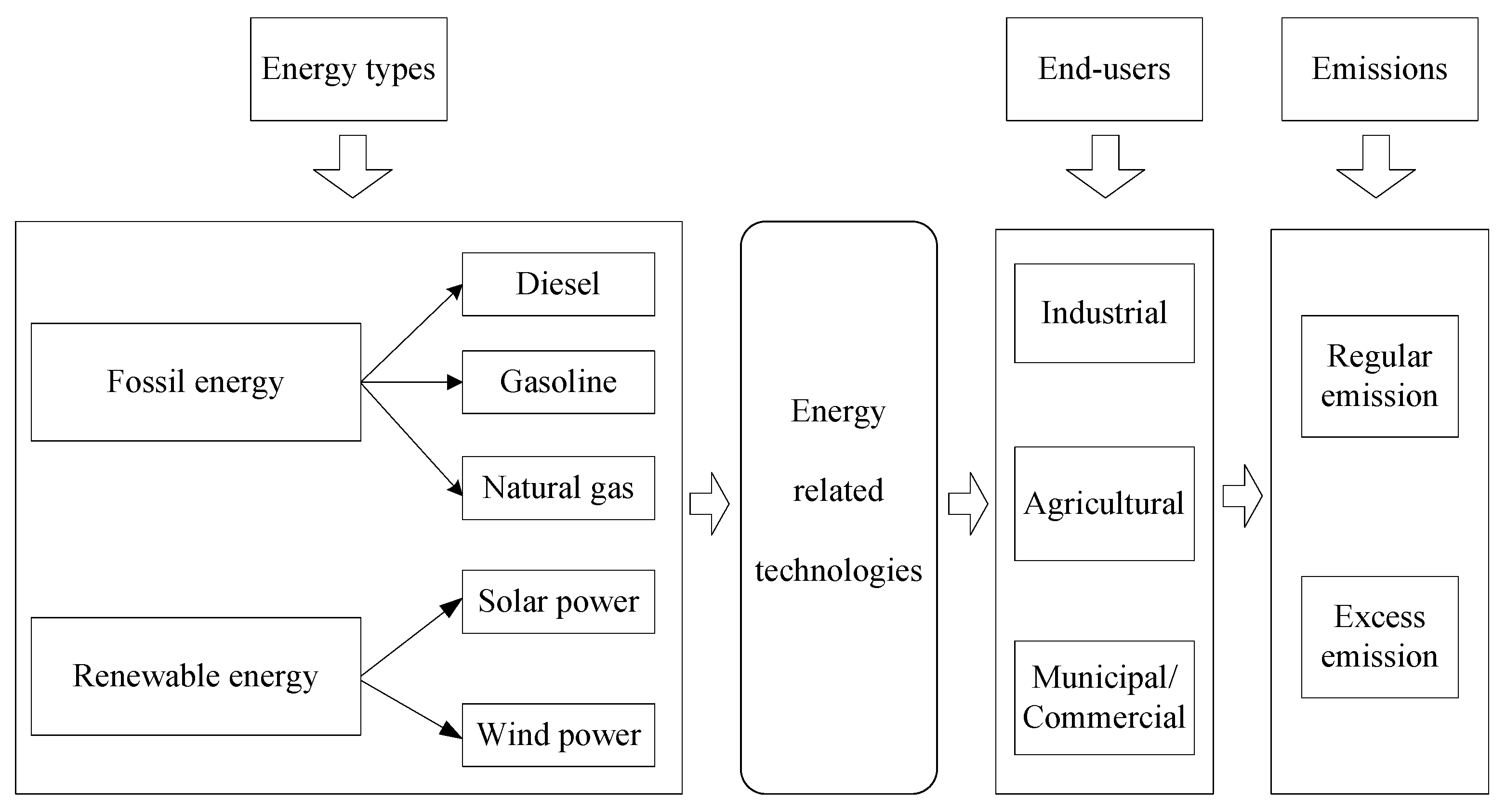
In this study, a hypothetical, but typical renewable energy management model is proposed for demonstrating the capability of the proposed optimization approach. The general structure of the proposed system is presented in Figure 1. The data are summarized through government reports and related literature, typical cost, and representative technical data are provided. The system contains multiple energy sources and technologies. Particularly, coal, diesel and natural gas are selected as typical fossil energy, while wind power and solar power are chosen as representative renewable energy. Decision makers should develop an effective plan to satisfy the industrial, agricultural and municipal energy demands. Regarding the environmental aspect, the power generation process will cause an inevitable pollution emission. SO₂ is chosen as the representative emission. Based on historical data, a predefined pollution control target is stipulated to each power generation facility. If the promised target is achieved, the unit could obtain certain profits as the net benefit. However, if an excess emission occurs, an economic penalty will be charged.

This study aims to develop an optimization integrate sensitive analysis model for supporting the scientific management of energy system by effectively dealing with the following problems: (1) Various types of uncertainties existed in the provided system, it should be reflected accurately and resolved effectively; (2) An optimal solution of energy activities should be obtained to balance the tradeoff between economic and environmental benefit, as well as the system stability. The results should include energy generation plan, technology selection result, and capacity expansion scheme; (3) The environmental control process should be represented. The related environmental factors would restrict the application of energy resources and technologies. For example, with a stricter policy, energy with lower emission rate or higher generation efficiency will be recommended. Correspondingly, it will provoke increased system cost; (4) The key impact factors and their potential interaction should be revealed. It would provide more detailed information for future decision making.

3.2. Stochastic Factorial Energy Systems Management Model

Therefore, the objectives of the study system are: (1) Arrange the five power conversion technologies effectively to meet the energy demands while maximizing the system benefits under uncertainty; (2) determine the minimum energy supply amount; (3) coordinate energy activities and environmental standard. Through the proposed method, a stochastic factorial energy systmes management model can be formulated. The objective function of the SFESM model can be expressed as follows:

$$\max f^{\pm }=f_1^{\pm }-f_2^{\pm }-f_3^{\pm }-f_4^{\pm }.$$

(35)

(1) System benefit related to environmental policy:

$$f_1^{\pm }={\displaystyle \sum _{i=1}^3{\displaystyle \sum _{t=1}^3\left(W{S}_{i,t}^{-}+\mathsf{\Delta }W{S}_{i,t}^{}\cdot p_{i,t}\right)\cdot CP{S}_{i,t}^{\pm }}}-{\displaystyle \sum _{i=1}^3{\displaystyle \sum _{m=1}^2{\displaystyle \sum _{t=1}^3\left(q_m\cdot Q{S}_{i,m,t}^{\pm }\cdot DP{S}_{i,t}^{\pm }\right)}}}.$$

(36)

(2) Cost for power generation

$$f_2^{\pm }={\displaystyle \sum _{i=1}^5{\displaystyle \sum _{t=1}^3\left(Y_{i,t}^{\pm }\cdot C{Y}_{i,t}^{\pm }\right)}}.$$

(37)

(3) Purchasing cost for primary energy supply

$$f_3^{\pm }={\displaystyle \sum _{i=1}^3{\displaystyle \sum _{t=1}^3\left(X_{i,t}^{\pm }\cdot C{X}_{i,t}^{\pm }\right)}}.$$

(38)

(4) Cost for capacity expansion

$$f_4^{\pm }={\displaystyle \sum _{i=2}^5{\displaystyle \sum _{n=1}^3\left(CE{Y}_{i,n}^{\pm }\cdot E{Y}_{i,n}^{\mp }\cdot Z{Y}_{i,n}^{\pm }\right)}}.$$

(39)

The net benefit is to be maximized by a series of constraints. The impact factors and their interactions are also provided. The detailed constraints are expressed as follows:

(1) Mass balance

$$X_{i,t}^{\pm }\ge V{Y}_{i,t}^{\pm }\cdot Y_{i,t}^{\pm }, \forall i=1,2,3;t,$$

(40)

(energy supply should be more than resource consumption)

(2) Availability of energy resources

$$Y_{i,t}^{\pm }\cdot F{E}_{i,t}^{\pm }\le X_{i,t}^{\pm }\cdot C{V}_i^{},\forall i=1,2,3;t,$$

(41)

$$Y_{i,t}^{\pm }\cdot F{E}_{i,t}^{\pm }\le A{V}_{i,t}^{\pm },\forall i=4,5;t,$$

(42)

(energy usage should be less than its availability)

(3) Electricity constraints

$${\displaystyle \sum _{i=1}^5{Y}_{i,t}^{\pm }}\ge {\displaystyle \sum _{j=1}^{3}DM{Y}_{j,t}^{\pm },} \forall t,$$

(43)

(electricity generation should be more than energy demands)

(4) Capacity limit

$$\left[R{Y}_i+{\displaystyle \sum _{n=1}^3\left(E{Y}_{i,n}^{}\cdot Z{Y}_{i,n}^{\pm }\right)}\right]\cdot UCAP{Y}_i^{\pm }\ge {\displaystyle \sum _{t=1}^3{Y}_{i,t}^{\pm }}, \forall i,$$

(44)

(installed capacity should be more than electricity generation)

(5) Constrains for controlling contamination

$${\displaystyle \sum _{i=1}^{5}V{Y}_{i,t}^{\pm }\cdot Y_{i,t}^{\pm }\cdot P{S}_i^{\pm }\cdot \left(1-{\eta }_i^{\pm }\right)}\le M{P}_t^{\pm },\forall t,$$

(45)

(SO₂ emission should be less than environmental standard)

$$\mathrm{Pr}\left\{{\displaystyle \sum _{i=1}^3\left(W{S}_{i,t}^{-}+\mathsf{\Delta }W{S}_{i,t}^{}\cdot p_{i,t}-Q{S}_{i,m,t}^{-}\right)\le C{P}_{m,t}^{},}\right\}\forall m,t,$$

(46)

(Actual SO₂ emission should be less than emission control target)

$$Q{S}_{i,m,t}^{\pm }\le W{S}_{i,t}^{-}+\mathsf{\Delta }W{S}_{i,t}^{}\cdot p_{i,t}\le W{S}_{i \max },\forall i,m,t,$$

(47)

(SO₂ generation amounts should be more than the excess amount, and less than given maximum)

$$Q{S}_{i,m,t}^{\pm }\ge 0,\forall i,m,t,$$

(48)

$$0\le p_{i,t}\le 1,\forall i,t.$$

(49)

(6) Technical constrains

$$X_{i,t}^{\pm }\ge 0,\forall i,t,$$

(50)

$$Y_{i,t}^{\pm }\ge 0,\forall i,t,$$

(51)

$$Z{Y}_{i,n}^{\pm }=\{\begin{array}{l}1,\mathrm{if}\mathrm{expansion}\mathrm{with}\mathrm{option}\mathrm{n}\mathrm{for}\mathrm{generating}\mathrm{technology}\mathrm{is}\mathrm{undertakan}\\ 0,\mathrm{otherwise}\end{array},$$

(52)

$$0\le {\displaystyle \sum _{n=1}^{3}Z{Y}_{i,n}^{\pm }}\le 1,\forall i,$$

(53)

$$0\le p_{i,t}\le 1.$$

(54)

The detailed nomenclatures for the variables and parameters are provided in the Appendix A. The research target is to maximize the system benefit under uncertainty. The developed energy model can be solved through the above method by decomposed into two deterministic sub-models. Specifically, the two-stage problem can be solved by letting $W{S}_{i,t}^{\pm }=W{S}_{i,t}^{-}+\mathsf{\Delta }W{S}_{i,t}^{}\cdot p_{i,t}$, where $\mathsf{\Delta }W{S}_{i,t}=W{S}_{i,t}^{+}-W{S}_{i,t}^{-}$. According to the Formulas (14)–(16) in Section 2.2, probability bounds of constraint violation under consideration are 1% and 10%. Transform the developed model into two sub-models, formulating the first sub-model which corresponds to $f_{opt}^{-}$. Then $Y_{opt}^{-},X_{opt}^{-},Z{Y}_{opt}^{-}$ can be obtained through the solution. Similarly, formulating the second sub-model corresponding to $f_{opt}^{+}$ and substituted calculated value above. Combine the two sub-models’ solutions to obtain the optimal solution of the proposed model. The data of energy activities are provided in

Table 1. Partial economic data of energy activities ^a.

Energy Resources	Period
	t = 1	t = 2	t = 3
Energy purchasing price ($/tonne)
Coal	[110, 120]	[105, 115]	[100, 110]
Diesel	[787, 798]	[782, 793]	[777, 788]
Natural gas	[720, 750]	[715, 745]	[710, 740]
Power generation ($/104 KW h)
Coal-fired	[52, 61]	[145, 53]	[39, 47]
Diesel-fired	[90, 112]	[75, 97]	[62, 82]
Gas-fired	[153, 167]	[136, 148]	[118, 130]
Wind power	[27, 36]	[22, 31]	[17, 26]
Solar power	[40, 48]	[35, 43]	[28, 38]

^a Adapted from References [21,26,34].

. Pollution treatment targets and the related economic data are given in

Table 2. Pollution treatment targets and related economic data.

	Source
	Coal-Fired	Diesel-Fired	Gas-Fired
Maximum pollution treatment amount (tonne)	7000	7000	7000
Commitment control target (tonne)	[5000, 6000]	[2800, 3800]	[130, 180]
Net benefit when commitment is satisfied (103 $/tonne)	[59, 79]	[51, 66]	[35, 45]
Penalty when commitment is not delivered (103 $/tonne)	[100, 140]	[110, 125]	[70, 105]

.

Furthermore, the factorial technique is introduced to a sensitive analysis of factor impact for system objective. It is predetermined that if energy activities meet the environmental standards, the specific regulation would affect net benefit directly. Therefore, factors related to pollution emission would have a more obvious influence on the evaluation of the system. The factorial design would then be simplified. It is not necessary to examine all system variables, only the factors relevant to the contamination control process should be taken into account. It would reduce the complexity of sensitive analysis and retrench the operation time. By factorial analysis technique, the key impact factors could be revealed. Meanwhile, it could demonstrate their potential interaction effect, which may have a greater impact on the system than individual variable. It would provide more detailed information for decision maker than traditional energy management methods. Future planning should be paid more attention to the key factors such as formulating stricter environmental standard or greater penalties.

3.3. Result Analysis

In this study, fifteen planning periods are considered, and each representative for one year. Through solving the developed model, the optimal primary energy supply scheme, electricity generation plan and conceivable capacity expansion options were generated. Solutions of contamination control and excess emission amount were calculated under different risk levels. It can demonstrate a basic tendency of energy activities and provide potential suggestions for policy development.

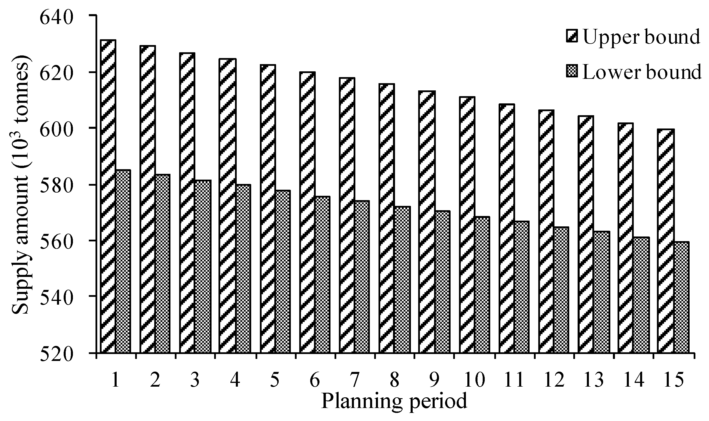
Figure 2 presents the purchasing plan for coal at each planning period. The result shows that the allocation amount had a visible downtrend over time. The allocated amount would decrease from [585.2, 631.4] × 10³ tonnes to [559.3, 599.7] × 10³ tonnes, fell about 4~5% during the fifteen years. It is in conformity with the basic requirement of a popular total amount control policy for coal. On the other hand, it also reveals that coal would still be the major energy source in the near future for its splendid reserve, extensive distribution, and shallow embedding. It means the coal usage should be on a declining trend yet would be less obvious. The non-renewable energy resources are a major component of energy supply in most cases. In this study, diesel and natural gas would also be selected to provide power to the end users. 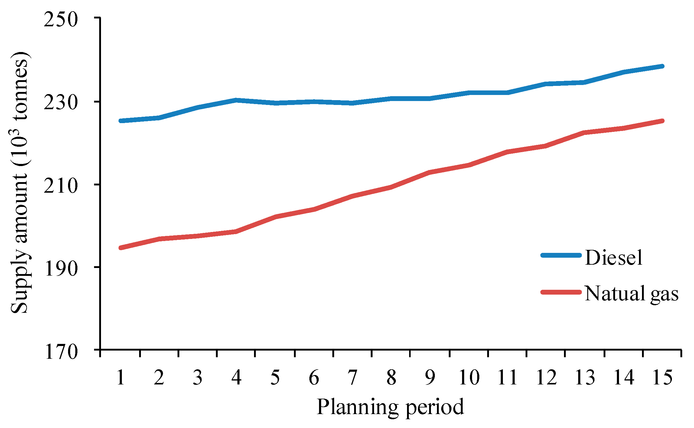Figure 3 provides the energy supply pattern of diesel and natural gas. The diesel supply would increase from 225.3 to 238.4 × 10³ tonnes during the planning period, while the deliverability of natural gas would increase from 194.8 to 225.4 × 10³ tonnes. The growth rate would be 5.8% and 15.7% respectively. The total purchasing amount of diesel and natural gas would be nearly half of coal. The allocated amount for diesel would be relatively stable. However, there’s a significant increase in natural gas. The difference between these two energy sources would be diminished over the planning period. If the tendency persists, natural gas may take coal’s place as the most favorite fuel in just a few decades. In a practical environment, according to BP statistical review of world energy, the world’s energy structure begins to diversify. It trends to increase thermal power generation by natural gas and decrease oil usage. That indicated the proposed case study could reflect the general trend thus provide useful information for policy making.

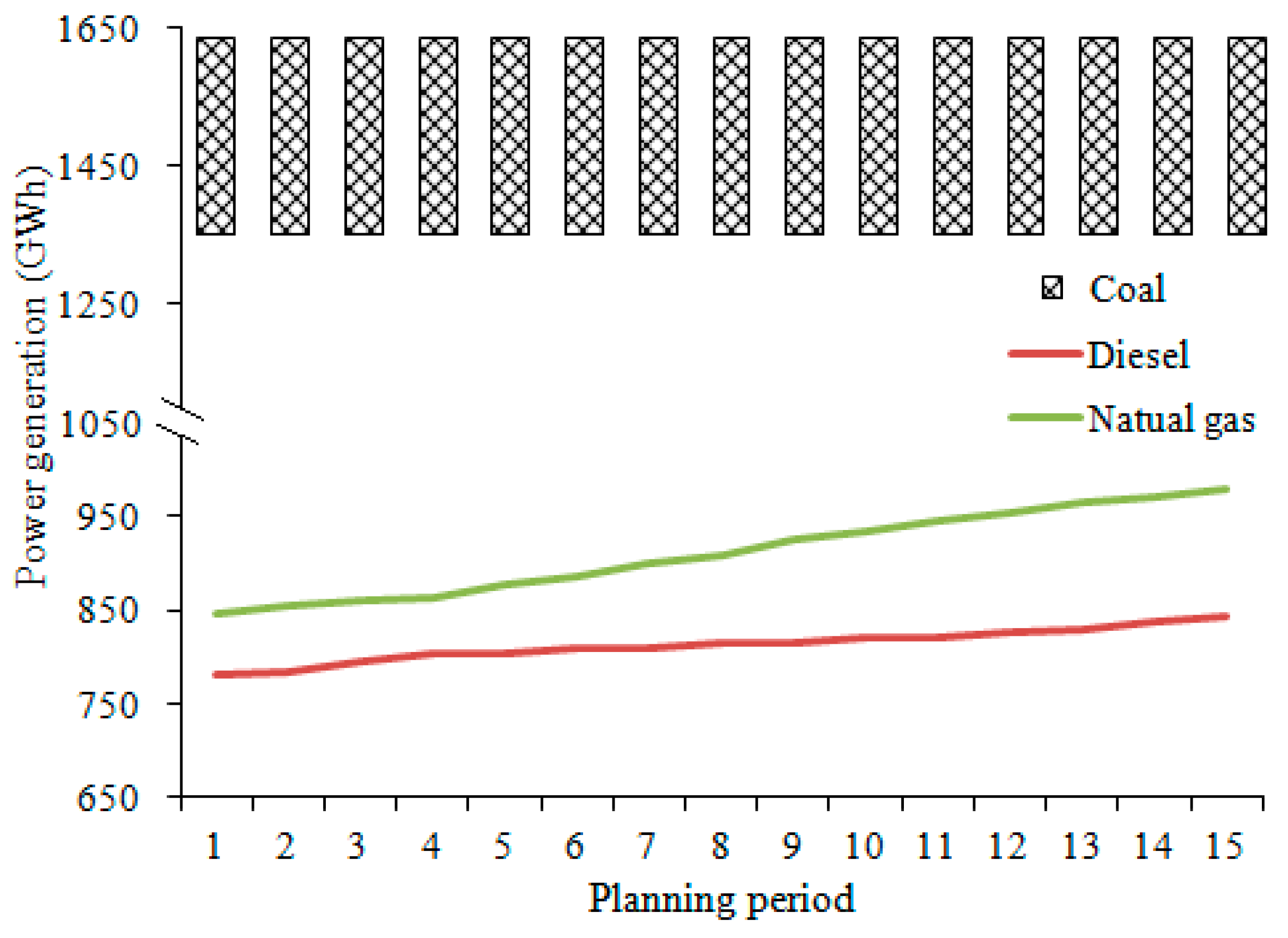
With the economy development, electrical power demand would increase every year. On the one hand, coal-fired power is the key factor in electricity generation activities. The efficiency for oil-based generators is close to coal, while the efficiency for natural gas-based generators would be almost twice higher. On the other hand, when emission control is considered, gas may be at least 25% cleaner than coal. From the environmental aspect, natural gas would be the optimal sources for energy supply. However, the operating cost for gas generators is much higher. Thus, it’s important to find a balance between them. Figure 4 presents the optimized solution of electricity generation plans of fossil energy. In detail, the energy generation by coal would be [1350.0, 1637.2] GWh over the planning horizon while the energy consumption would slightly decrease. Diesel and gas-fired power would be markedly increased. The electricity generated by diesel would range from 780.4 to 842.5 GWh. Gas based electricity would increase from 847.0 GWh to 979.9 GWh, and the median would be 900.7 GWh. The growth rate for gas-fired power would be 15.7%, while the growth for diesel was modest. In this study, renewable energy sources were also employed. In this study, renewable energy sources were also considered. The installed capacities for wind/solar power were set under 50 MW, since the large-scale applications of renewable energy are still not mature and the maintenance costs are much higher (Table 1). The initially installed capacities for fossil energy were set to 300 MW. It turns out that contribution rate for renewable energy would be 1%. Among them, wind power would occupy 58%, while solar energy would be 42%. The results of power generation pattern are provided in Figure 5 The result also shows that they could meet the demands of end-users; hence capacity expansion would not be needed.

Normally, a predefined SO₂ treatment target is promised to meet the environmental standards. If the commitment amounts are not delivered, due to the insufficient pollution control availabilities, excess emission will occur thus cause penalty for the system benefit. Under normal circumstances, the pre-regulated amounts will meet the demand. The higher probability is formulated for this case. However, some artificial subjective reasons like budgeting control or some uncontrollable factors, pollution treatment facilities are not effectively operated. It could affect pollution treatment availabilities. Therefore, a relatively lower probability is provided. In optimization studies, constraints could be partially satisfied. In order to obtain a more acceptable result, constraint violation may be allowed at certain risk levels. In this study, two risk levels were set to 0.01 and 0.1, respectively. Correspondingly, each represents the satisfaction degree for the constraints should be at least 99% or 90%. The detailed information is provided in

Table 3. Pollution control availabilities under different risk levels (tonne).

	Pollution Control Availability (CPm,t)	Risk Level
		α = 0.01	α = 0.10
Lower probability	N (2850, 150)	2051	2658
Higher probability	N (6250, 150)	5901	6058

.

Solutions were generated for pollution control recommendations. As shown in

Table 4. Solutions obtained for the objective function and decision variables (tonnes).

	Probability (qm)	Source
		Coal-Fired	Diesel-Fired	Gas-Fired
Target WSiopt		5000	2800	180
Risk level α = 0.01
Excess emission (QS) under the level of
Low (m=1)	40%	5000	299	180
High (m=2)	60%	1899	0	180
Treated amount under the level of
Low (m=1)	40%	0	2501	0
High (m=2)	60%	3101	2800	0
Risk level α = 0.10
Excess emission (QS) under the level of
Low (m=1)	40%	5000	142	180
High (m=2)	60%	1742	0	180
Treated amount under the level of
Low (m=1)	40%	0	2658	0
High (m=2)	60%	3258	2800	0

, optimized target treatment amounts were firstly obtained for three sources. The solutions of WS_iopt revealed that the optimal treatment targets would be 5.0 × 10³ tonnes for SO₂ generated by the burning of coal, 2.8 × 10³ tonnes for diesel-fired SO₂, and 180 tonnes for gas-fired SO_2, respectively. The existing SO₂ processing capacity could not meet requirements, excess emission occurred at both risk levels. For risk level at 0.01, when the availability is relatively low with a probability of 40%, excess emission for the three sources would be 5.0, 0.3 and 0.2 × 10³ tonnes, respectively; when the availability is higher with a probability of 60%, excess SO₂ emission for coal and natural gas would be 1.9 and 0.2 × 10³ tonnes, while no excess emission would occur for diesel-based power plant. For risk level at 0.1, the availability increases under this circumstance. Generally, with stricter environmental policies, excess emission would decrease. When at the lower probability, excess emission for diesel-fired plants would drop to 0.1 × 10³ tonnes; while at the higher probability, excess emission for coal-based plants would drop to 1.7 × 10³ tonnes. Other data would be unchanged at two risk levels. The results also indicate that when pollution treatment availability is insufficient, the SO₂ produced by diesel plants would be firstly treated, and secondly for coal-fired plants. This is because the penalty for diesel-fired pollution is the highest and the relevant units could also bring substantial benefit. For gas-fired plants, SO₂ discharge would not be controlled, since the total amount is quite small. The actual treated amount for each type of power plant at different risk levels can be calculated from treatment targets and excess emissions, all the results are also expressed in Table 4.

To address uncertainties in a thorough manner and provide a comprehensive outcome, a further sensitive analysis is necessary. The object of the proposed system is to address the maximum net benefits while meeting the constraints. It is important to reveal the main factors related to the study objectives. Factorial analysis is therefore introduced to examine these uncertain parameters and their interactions. In this study, the system benefit is calculated based on emission production amount, while the penalty will be taken when violated the environmental policy. Thus, seven factors related to the pollution control process are selected. These factors are donated as A, B, C, D, E, F and G. All the factors are presented at two levels. For factors A: F, they refer to the lower and upper bound of the chosen variable, since they are all interval numbers. For factor G, they represent the two risk levels.

Table 5. Investigated factors with two levels.

Factor	Name	Units	Level
			Low	High
A	CPS1: Regular operating cost for SO2 generated by coal	$/tonne	59	79
B	CPS2: Regular operating cost for SO2 generated by diesel	$/tonne	51	66
C	CPS3: Regular operating cost for SO2 generated by natural gas	$/tonne	35	45
D	DPS1: Penalty cost for excess emission generated by coal	$/tonne	200	240
E	DPS2: Penalty cost for excess emission generated by diesel	$/tonne	270	320
F	DPS3: Penalty cost for excess emission generated by natural gas	$/tonne	240	300
G	Risk level		0.01	0.1

shows all the selected uncertain parameters. The proposed two-level factorial design with seven factors would require 128 experimental runs. The major purpose of this design would be verifying and evaluating the factors influencing on total system benefits.

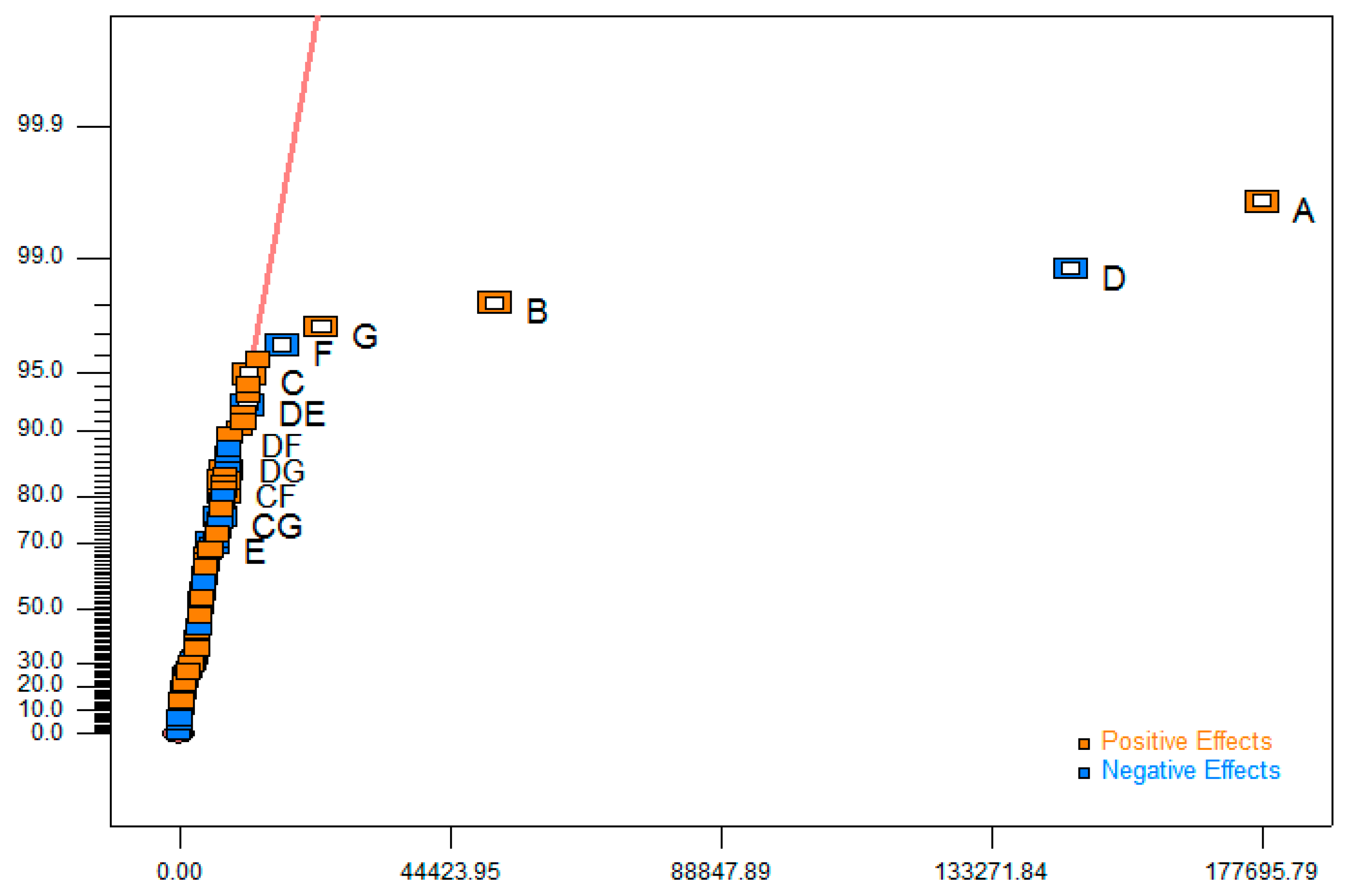
Figure 6 presents the half-normal plot of the effects of all the factors. The plot is an effective graphical technique to help identify the key factors. The larger the distance represents the more significant impact of the factor. The yellow outcome represents positive effects, which means increasing the net benefits. Correspondingly, the blue square representing penalty to the system. The results indicate that factors A, D, B and G would be the key effect factors. Besides, for some interaction factors, the effect is significant. For example, the effects for interaction DE, DF, DG, CF and CG are higher than the main effect of factor E. It implies that an important interrelationship may exist between the factors and their interaction plot should therefore be analyzed.

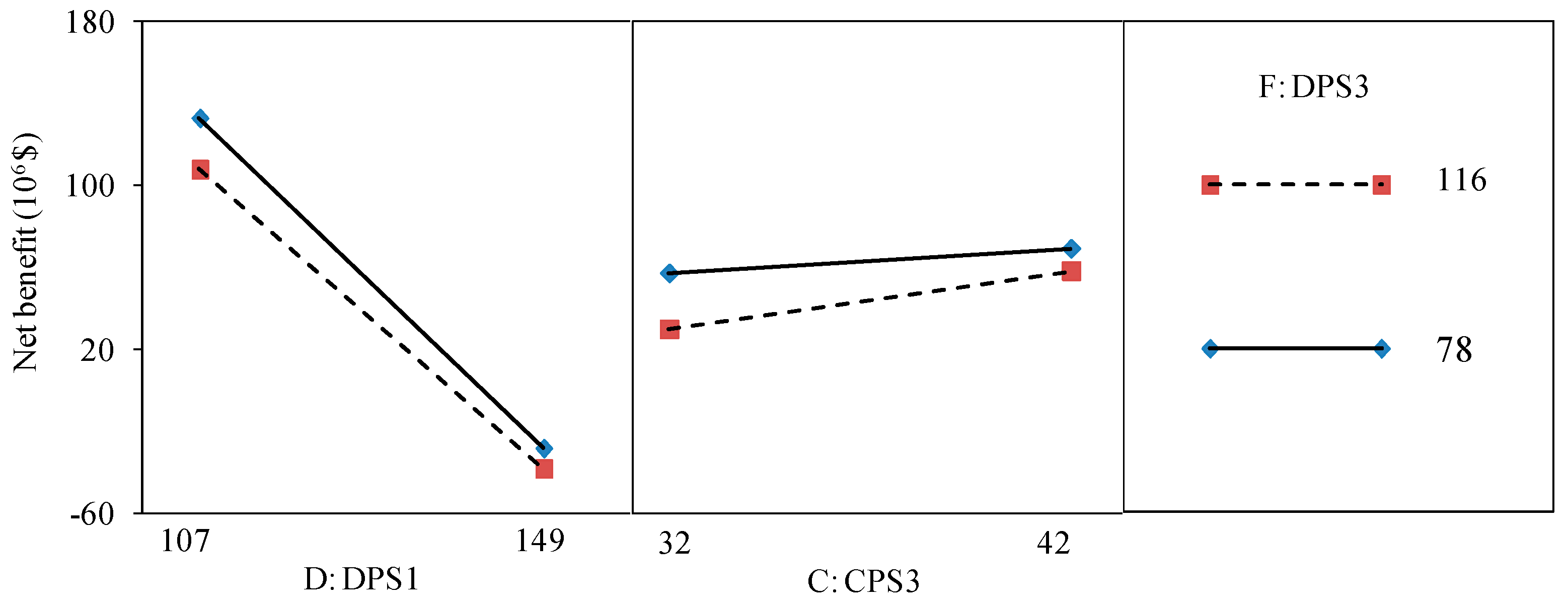
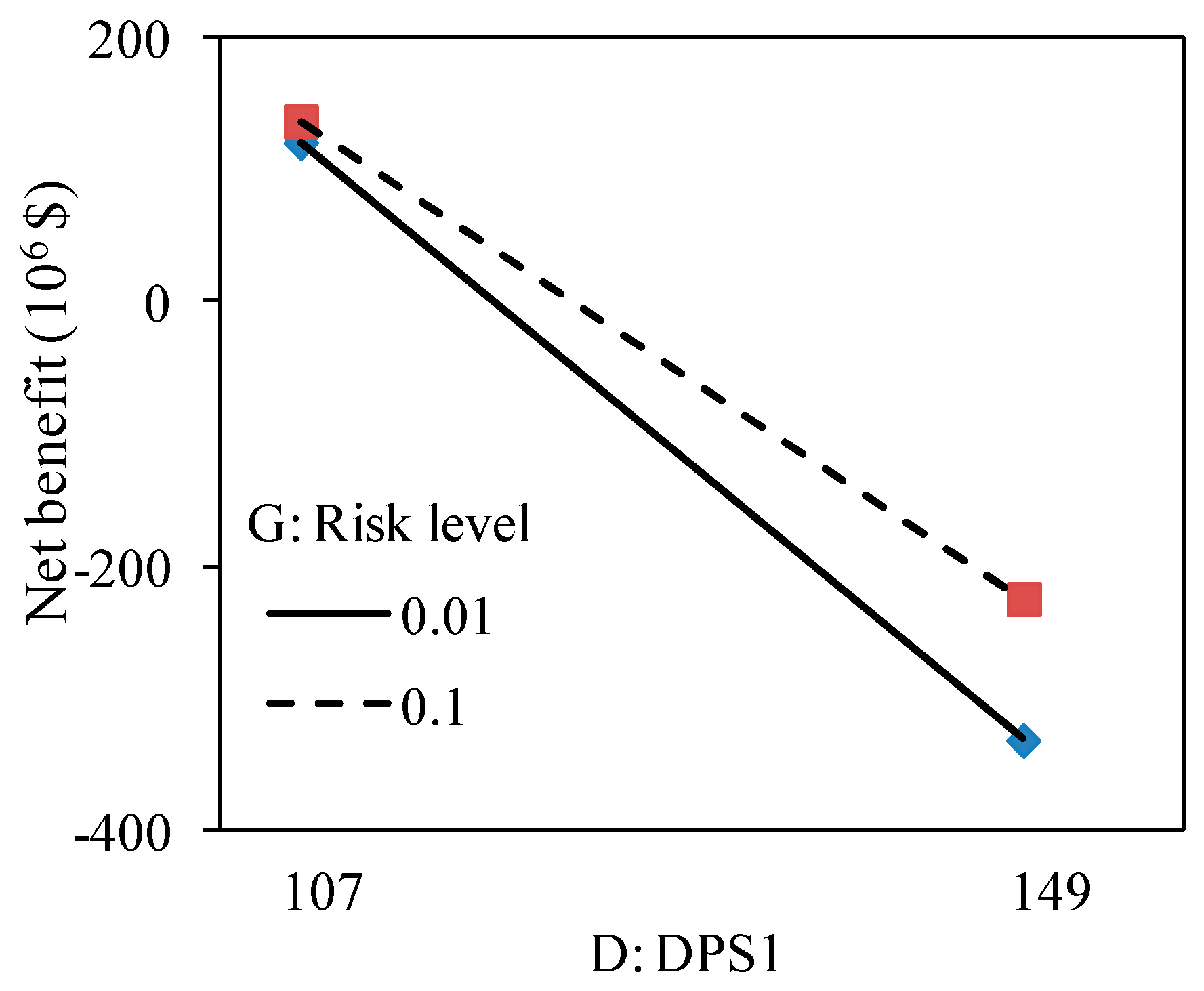
Figure 7 provides the interaction plot of factors D and E. It implies that the factor D would have a negative effect on the net benefit. When the value for factor D approach to its upper bound, the total revenue of the system will decrease gradually. This trend would become more prominent when factor E is at its higher bound. Figure 8 presents the interactions plot matrix for factor C/D with F. It indicates that factor C would have a positive effect on the system, but the impact is unapparent. The impact of factor D would become more significant with F at the lower bound, while the impact of C would be more obvious when F at the upper bound. Similarly, Figure 9 shows the interaction plot of factors D and G. It states that the impact of factor D would become more significant when G is at the lower level. The results show that system benefits would be improved with a higher violation risk. When the profits surpass the punishment, it would contribute significantly to excess emission. That indicates that policies regarding the environment will not be loosened in order to allow more profits to pass environmental examinations. It reveals the tradeoffs between conflicting economic development and environment protection. It is a very important responsibility for decision makers to protect the environment during economics developing.

To demonstrate the superiority of the proposed method, a compared result is obtained with a traditional deterministic method. The proposed energy management system contains multiple planning affairs and multiple risk levels, due to the space limitation, only electricity generation plans with risk level α = 0.1 is emphasized in

Table 6. Compared electricity generation result under risk level α = 0.1.

	Coal	Diesel	Natural Gas	Wind Power	Solar Power
Proposed method	[1350.0, 1637.2]	[780.4, 842.5]	[847.0, 979.9]	[14.3, 20.5]	[8.3, 14.9]
Deterministic method	1500	1500	121	17	12

. The programming approach was solved by replacing the uncertain variables with their mid-point values. Differing from the proposed method, with various uncertain inputs, the application of deterministic programming can only provide a single response. In realistic energy system planning, an accurate value could hardly provide the guidance for decision makers. Similarly, by solving the maximum and minimum values of the uncertain parameters, solutions under best/worst scenarios can be obtained. It can be used for judging the capability of the system, but hardly establish a stable interval for policy or strategy. Besides, the further sensitive analysis could be employed, but solutions of the deterministic method cannot reveal the interaction effects among different factors. Thus, it hardly provides useful analysis for decision variables.

Generally, the above analysis indicates that solutions of the SFESM model can provide an effective relevance with pre-regulated energy policies and the related penalties. It facilitates the settlement of multiple types of uncertainties. Optimal primary energy supply, electricity generation, capacity expansion and pollution control plans are generated. The interval results under different risk levels are operable and can help decision makers obtain diversified decision alternatives. Besides, techniques of sensitive analysis can be applied for supporting the further adjustment of the optimization model and promoting the commonality to the practical situation.

4. Conclusions

In this study, a stochastic factorial programming is proposed for reforming regional energy structure management, and conducting uncertainties and risks, as well as handle their interaction effects among different environmental policies in the energy systems. The proposed method is able to tackle uncertainties expressed as interval values and probability distributions and can be further used for examining all possible decision options which have relevance to various levels of economic penalties if the proposed policy targets are violated. Optimal decisions of emission control schemes, primary energy supply, electricity generation, and capacity expansion can be generated. Particularly, it can help examine uncertain parameters and their interactions to analyze their impact on the system performance through factorial analysis. Compared with the conventional energy and environmental systems management, the proposed method could not only handle the uncertainties expressed as interval and random variables, but also provide more specific results of parameter effects and their potential interactions on the system performance.

The developed method has been applied to a case of environmentally-friendly oriented planning of renewable energy system management system within a multi-facility, multi-period and multi-demand-level context. This study identified significant factors (e.g., environmental control factors) and reflected their interactions in the energy management model. It proves that reducing coal usage through economic measures would be not effective, policies like total quantity control of coal are necessary to reduce SO₂ emissions. The results indicated that the proposed method would incorporate significant uncertain information into the decision-making process and capture a technically feasible solution at different levels of system reliability. The results can be used for supporting the adjustment for allocation of energy resources, analyzing the tradeoff between conflicting economic and environmental objectives and formulating the local policies.

The proposed method still has limitations, since factors with multiple levels could exist in large scale energy systems management. It, thus, suggests introducing mix-level factorial analysis into the framework. Further optimization methods could also be added to address the uncertainties within the system. This will then extend the approach and facilitate further application.

References

1. Yao, L.; Wang, X.; Qian, T.; Qi, S.; Zhu, C. Robust day-ahead scheduling of electricity and natural gas systems via a risk-averse adjustable uncertainty set approach. Sustainability 2018, 10, 3848. [Google Scholar] [CrossRef]
2. Shen, Y.; Tan, Z.; Shen, X.; Bai, J.; Li, Q.; Wang, S. Study of energy saving and emission reduction based on the OLAP multi-indicator relational model. J. Environ. Inform. 2012, 20, 115–122. [Google Scholar] [CrossRef]
3. Suo, M.; Li, Y.; Huang, G.; Deng, D.; Li, Y. Electric power system planning under uncertainty using inexact inventory nonlinear programming method. J. Environ. Inform. 2013, 22, 49–67. [Google Scholar] [CrossRef]
4. Khare, A.R.; Kumar, B.R. Multiagent structures in hybrid renewable power system: A review. J. Renew. Sustain. Energy 2015, 7, 063101. [Google Scholar] [CrossRef] [Green Version]
5. Pettersson, F. Carbon pricing and the diffusion of renewable power generation in Eastern Europe: A linear programming approach. Energy Policy 2007, 35, 2412–2425. [Google Scholar] [CrossRef]
6. Gilau, A.M.; Van Buskirk, R.; Small, M.J. Enabling optimal energy options under the Clean Development Mechanism. Energy Policy 2007, 35, 5526–5534. [Google Scholar] [CrossRef]
7. Zhang, Q.; Wei, H.; Zhao, Z.; Liu, J.; Ran, Q.; Yu, J.; Gu, W. Optimization of the fuzzy matter element method for predicting species suitability distribution based on environmental data. Sustainability 2018, 10, 3444. [Google Scholar] [CrossRef]
8. Lee, M.; Lee, J.; Lee, J.; Kim, Y.; Park, Y.; Lee, K. Uncertainty analysis of a GHG emission model output using the block bootstrap and monte carlo simulation. Sustainability 2017, 9, 1522. [Google Scholar] [CrossRef]
9. Mellit, A.; Benghanem, M.; Kalogirou, S.A. Modeling and simulation of a stand-alone photovoltaic system using an adaptive artificial neural network: Proposition for a new sizing procedure. Renew. Energy 2007, 32, 285–313. [Google Scholar] [CrossRef]
10. Sheng, W.; Peng, S.; Tang, Y.; Meng, X.; Wang, D.; Wu, Z.; Gu, W. Stochastic multi-objective scheduling of a combined cooling, heating and power microgrid containing a fuel cell. J. Renew. Sustain. Energy 2015, 7, 063123. [Google Scholar] [CrossRef]
11. Florides, G.A.; Kalogirou, S.A.; Tassou, S.A.; WrobelL, C. Modeling of the modern houses of Cyprus and energy consumption analysis. Energy 2000, 25, 915–937. [Google Scholar] [CrossRef]
12. Li, Y.; Huang, G.; Veawab, A.; Nie, X.; Liu, L. Two-stage fuzzy-stochastic robust programming: A hybrid model for regional air quality management. J. Air Waste Manag. Assoc. 2006, 56, 1070–1082. [Google Scholar] [CrossRef] [PubMed]
13. Ajorlou, A.; Moezzi, K.; Aghdam, A.; Tafazoli, S.; Nersesov, S. Two-stage energy-optimal formation reconfiguration strategy. Automatica 2012, 48, 2587–2591. [Google Scholar] [CrossRef]
14. Moradzadeh, B.; Tomsovic, K. Two-stage residential energy management considering network operational constraints. IEEE Trans. Smart Grid 2013, 4, 2339–2346. [Google Scholar] [CrossRef]
15. Lin, Q.; Huang, G. An inexact two-stage stochastic energy systems planning model for managing greenhouse gas emission at a municipal level. Energy 2010, 35, 2270–2280. [Google Scholar] [CrossRef]
16. Charnes, A.; Cooper, W. Chance-constrained programming. Manag. Sci. 1959, 6, 73–79. [Google Scholar] [CrossRef]
17. Udhayakumar, A.; Charles, V.; Kumar, M. Stochastic simulation based genetic algorithm for chance constrained data envelopment analysis problems. Omega 2011, 39, 387–397. [Google Scholar] [CrossRef]
18. Fleten, S.E.; Kristoffersen, T.K. Short-term hydropower production planning by stochastic programming. Comput. Oper. Res. 2008, 35, 2656–2671. [Google Scholar] [CrossRef]
19. Rong, A.; Lahdelma, R. CO2 emissions trading planning in combined heat and power production via multi-period stochastic optimization. Eur. J. Oper. Res. 2007, 176, 1874–1895. [Google Scholar] [CrossRef]
20. Wang, Z.; Huang, G.; Cai, Y.; Dong, C.; Sun, H. The Identification of optimal CO2 emissions-trading strategies based on an inexact two-stage chance-constrained programming approach. Int. J. Green Energy 2014, 11, 302–319. [Google Scholar] [CrossRef]
21. Cai, Y.; Huang, G.; Yang, Z.; Lin, Q.; Tan, Q. Community-scale renewable energy systems planning under uncertainty—An interval chance-constrained programming approach. Renew. Sustain. Energy Rev. 2009, 13, 721–735. [Google Scholar] [CrossRef]
22. Cheng, X.; Fan, L.; Wang, J. Can energy structure optimization, industrial structure changes, technological improvements, and central and local governance effectively reduce atmospheric pollution in the Beijing–Tianjin–Hebei Area in China? Sustainability 2018, 10, 644. [Google Scholar] [CrossRef]
23. Lewis, S.M.; Dean, A.M. Detection of interactions in experiments on large numbers of factors. J. R. Stat. Soc. Ser. B (Stat. Methodol.) 2001, 63, 633–672. [Google Scholar] [CrossRef] [Green Version]
24. Lin, Y.; Huang, G.; Lu, H.; He, L. A simulation-aided factorial analysis approach for characterizing interactive effects of system factors on composting processes. Sci. Total Environ. 2008, 402, 268–277. [Google Scholar] [CrossRef] [PubMed]
25. Zhou, Y.; Huang, G. Factorial two-stage stochastic programming for water resources management. Stoch. Environ. Res. Risk Assess. 2011, 25, 67–78. [Google Scholar] [CrossRef]
26. Liu, Z.; Huang, G.; Li, W. An inexact stochastic–fuzzy jointed chance-constrained programming for regional energy system management under uncertainty. Eng. Optim. 2015, 47, 788–804. [Google Scholar] [CrossRef]
27. Wang, S.; Huang, G. A multi-level Taguchi-factorial two-stage stochastic programming approach for characterization of parameter uncertainties and their interactions: An application to water resources management. Eur. J. Oper. Res. 2015, 240, 572–581. [Google Scholar] [CrossRef]
28. Xin, X.; Huang, G.; Sun, W.; Zhou, Y.; Fan, Y. Factorial two-stage irrigation system optimization model. J. Irrig. Drain. Eng. 2015, 142, 04015056. [Google Scholar] [CrossRef]
29. Onsekizoglu, P.; Bahceci, K.S.; Acar, J. The use of factorial design for modeling membrane distillation. J. Membr. Sci. 2010, 349, 225–230. [Google Scholar] [CrossRef]
30. Wang, S.; Huang, G.; Veawab, A. A sequential factorial analysis approach to characterize the effects of uncertainties for supporting air quality management. Atmos. Environ. 2013, 67, 304–312. [Google Scholar] [CrossRef]
31. Zhou, Y.; Huang, G.; Yang, B. Water resources management under multi-parameter interactions: A factorial multi-stage stochastic programming approach. Omega 2013, 41, 559–573. [Google Scholar] [CrossRef]
32. Yeomans, J.S.; Huang, G. An evolutionary grey, hop, skip, and jump approach: Generating alternative policies for the expansion of waste management facilities. J. Environ. Inform. 2003, 1, 37–51. [Google Scholar] [CrossRef]
33. Yeomans, J.S.; Huang, G.; Yoogalingam, R. Combining simulation with evolutionary algorithms for optimal planning under uncertainty: An application to municipal solid waste management planning in the regional municipality of Hamilton-Wentworth. J. Environ. Inform. 2003, 2, 11–30. [Google Scholar] [CrossRef]
34. Zhu, Y.; Li, Y.; Huang, G. Planning carbon emission trading for Beijing’s electric power systems under dual uncertainties. Renew. Sustain. Energy Rev. 2013, 23, 113–128. [Google Scholar] [CrossRef]
35. Li, Y.; Li, Y.; Huang, G.; Chen, X. Energy and environmental systems planning under uncertainty—an inexact fuzzy-stochastic programming approach. Appl. Energy 2010, 87, 3189–3211. [Google Scholar] [CrossRef]
36. Charnes, A.; Cooper, W.; Kirby, M. Chance-Constrained Programming: An Extension of Statistical Method; No. CS-59; Texas University Austin Center for Cybernetic Studies: Austin, TX, USA, 1971. [Google Scholar]
37. Infanger, G.; Morton, D.P. Cut sharing for multistage stochastic linear programs with interstage dependency. Math. Program. 1996, 75, 241–256. [Google Scholar] [CrossRef]
38. Charnes, A.; Cooper, W.; Golany, B.; Seiford, L.; Stutz, J. Foundations of data envelopment analysis for Pareto-Koopmans efficient empirical production functions. J. Econom. 1985, 30, 91–107. [Google Scholar] [CrossRef]
39. Ellis, J.H.; Zimmerman, J.J.; Corotis, R.B. Stochastic programs for identifying critical structural collapse mechanisms. Appl. Math. Model. 1991, 15, 367–373. [Google Scholar] [CrossRef] [Green Version]
40. Infanger, G. Monte Carlo (importance) sampling within a Benders decomposition algorithm for stochastic linear programs. Ann. Oper. Res. 1992, 39, 69–95. [Google Scholar] [CrossRef]
41. Watanabe, T.; Ellis, H. A joint chance-constrained programming model with row dependence. Eur. J. Oper. Res. 1994, 77, 325–343. [Google Scholar] [CrossRef]
42. Zare, Y.; Daneshmand, A. A linear approximation method for solving a special class of the chance constrained programming problem. Eur. J. Oper. Res. 1995, 80, 213–225. [Google Scholar] [CrossRef]
43. Huang, G.; Baetz, B.W.; Patry, G.G. A grey linear programming approach for municipal solid waste management planning under uncertainty. Civ. Eng. Syst. 1992, 9, 319–335. [Google Scholar] [CrossRef]
44. Huang, G.; Loucks, D.P. An inexact two-stage stochastic programming model for water resources management under uncertainty. Civ. Eng. Syst. 2000, 17, 95–118. [Google Scholar] [CrossRef]
45. Box, G.E.; Hunter, W.G.; Hunter, J.S. Statistics for Experimenters: An Introduction to Design, Data Analysis, and Model Building; Wiley: New York, NY, USA, 1978. [Google Scholar]
Figure 1. Interactive relationships of the energy system.
Sustainability 11 02429 g001
Figure 2. Energy purchasing plan for coal at each planning period.
Sustainability 11 02429 g002
Figure 3. Comparison result of energy purchasing plan for diesel and natural gas.
Sustainability 11 02429 g003
Figure 4. Electricity generation plans of fossil energy-based power plant.
Sustainability 11 02429 g004
Figure 5. Electricity generation pattern.
Sustainability 11 02429 g005
Figure 6. Half-normal plot of the effects.
Sustainability 11 02429 g006
Figure 7. Interaction plot of factors D and E.
Sustainability 11 02429 g007
Figure 8. Interaction plot of factors C/D with F.
Sustainability 11 02429 g008
Figure 9. Interaction plot of factors D and G.
Sustainability 11 02429 g009