Investigating the Energy-Environmental Kuznets Curve Hypothesis for the Asia-Pacific Region

Abstract

As mitigating the effects of energy consumption on the environment is a crucial issue for the Asia-Pacific region, this study investigates the energy-environmental Kuznets curve (EEKC) hypothesis among the 19 Asia-Pacific countries. The study also tests the EEKC hypothesis for the low-, middle-, and high-income groups of the region. The panel regression and cointegration models are used for this purpose. Our test results of both models suggest that the EEKC hypothesis holds for the whole Asia-Pacific region. However, the test performed on the three different income groups revealed that the hypothesis only holds for the high-income group. The hypothesis was not apparent for the low- and middle-income groups. This indicates that the transition in the energy consumption along the EEKC is only occurring in the developed countries of the Asia-Pacific region and the developed countries need to support the developing countries to achieve economic growth along the EEKC.

1. Introduction

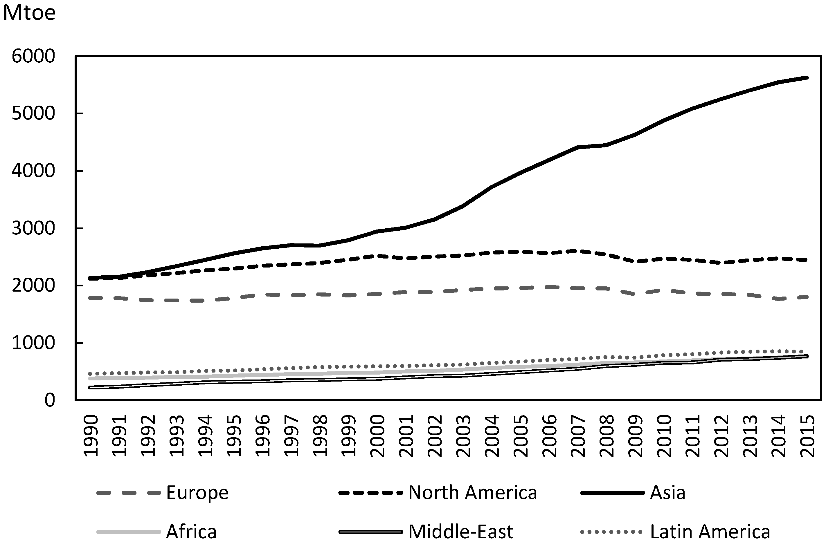
Since the beginning of this century, the level of energy consumption in Asia has been growing at an unprecedented speed (see Figure 1) and now Asia is the world’s largest energy consumer. As the current climate change is largely related to the anthropogenic emissions of carbon dioxide resulted from increased fossil fuel energy use [1] (p.136), this surge in the energy consumption in Asia is increasingly placing pressure on the environment. Consequently, Asian countries need to find ways for sustainable development, reducing fossil fuel energy consumption while attaining economic growth. However, new and less cost-efficient technologies that can perfectly substitute fossil fuel energy is still unavailable, and currently, an increase in energy consumption is connected to increased fossil fuel energy use. This is contributing to global warming and it is becoming crucial for countries to achieve economic development using energy in a more efficient way. Hence, more studies need to be done to understand the relationship between economic growth and energy consumption.

Studies traditionally investigating economic growth and energy relationships do not identify the quadratic relationship between energy consumption and economics growth because most of these studies are only interested in their causal relationships [2]. However, recently, it is becoming a trend to test the relationship between energy consumption and economic growth under the environmental Kuznets curve (EKC) hypothesis [3,4,5]. This is because scholars started to realize the importance of considering the pressure of energy consumption on the environment when achieving sustainable development. The concept of the EKC hypothesis emerged in the early 1990s with Grossman and Krueger [6] and the name EKC was first introduced by Panayotou [7]. EKC hypothesis states that there is an inverted U-shape relationship between economic development and environmental degradation. Since the early 1990s, many empirical studies found that an environmental pressure becomes smaller once a certain level of economic growth is achieved when there is a shift from fossil fuel energy-intensive industry to one not dependent much on fossil fuel energy [8,9,10].

Recently, studies have started to use this EKC model to examine the relationship between energy consumption and economic development because energy consumption is becoming a serious factor in causing pressure on the environment. Indeed, up until now, most of the energy use in the world relies on fossil fuel energy, and an increase in energy consumption is one of the major contributors to the amplification of greenhouse gas emissions.

Although many studies have investigated the energy-environmental Kuznets curve (EEKC) hypothesis for the whole world, only a few studies exist that examine this hypothesis focusing on a specific region. A study of Pablo-Romero and De Jesús [11] is among those few testing the hypothesis for Latin America, but there are very few studies focusing on the Asian region. As far as we know, there exist studies analyzing the environmental Kuznets curve hypothesis for the Asian region [12,13], but up until now, no studies have investigated the EEKC hypothesis for this region.

To fill this gap, this study examines whether the EEKC hypothesis holds in the Asia-Pacific region during the 1984–2014 period. The EEKC hypothesis investigated in this study is that there is an inverted U-shape relationship between the income level and energy consumption in the Asia-Pacific region. In the study, we use data for 19 countries that belong to the Asia-Pacific region. If we verify that the EEKC hypothesis holds for the region, we also estimate the income level at the turning point of its energy consumption.

Whether the Asia-Pacific region follows the EEKC hypothesis depends on how the level of energy consumption shifts along the GDP per capita of the region. For example, if the region’s economic growth depends highly on energy use, it is less likely that we find any decline in its energy consumption with GDP per capita. On the other hand, if the region is adopting energy-saving technology that reduces its energy use with GDP per capita growth, the region is likely to satisfy the EEKC hypothesis.

Analyzing the EEKC hypothesis for the Asia-Pacific region is particularly interesting because this region contains both developing and developed countries and it is a region on the verge of energy transition. If we find that an EEKC hypothesis holds in this region, it would imply that there is an energy transition at some point where the energy consumption starts to decline as its economy grows. When this is the case, it is likely that the economic growth of this region does not increase the regional energy consumption and cause environmental pressure. However, if the study indicates denial of the EEKC hypothesis, it will suggest that there is no turning point for energy use in the region. In this case, it will mean that economic growth does not help reduce energy consumption in the region and economic growth will intensify the greenhouse effects. Then, the study will indicate the importance of enhancing energy saving technology in the region to mitigate the effects of economic growth on the environment.

In the next section, we briefly show some previous studies testing the EEKC hypothesis. In the third section, we discuss the methods and data of this study. The fourth section reveals the results of the analyses performed in the study. Finally, in the last section, we provide discussions and conclusions.

2. Previous Studies

Many studies have investigated the relationship between economic growth and energy consumption [2,14,15] but most of these studies do not examine this relationship in the context of the EKC hypothesis.

Suri and Chapman [3] is one of the early studies to test the EKC hypothesis with respect to energy consumption itself. Before this study, most of the studies investigating the energy EKC hypothesis did not use the data for energy consumption and applied energy-related pollutants to represent environmental pressures. Suri and Chapman [3] use the energy consumption and GDP data for the 33 countries of all parts of the world over the 1971–1991 period. They find that the downturn in the inverted-U curve is related to the change in the trades of manufactured goods. They conclude that the increase in the imports of the manufactured goods plays an important role in reducing the energy use of a country.

Luzzati and Orsini [4] also perform a study to analyze the relationship between energy consumption and GDP per capita to identify the existence of the EKC hypothesis. They used data for 113 countries including the oil producing countries over the 1971–2001 period and find no evidence of an inverted-U pattern between the energy consumption and GDP per capita.

Chen et al. [5] examine the relationships among economic growth, energy consumption, and CO₂ emissions for 188 countries in the world for the 1993–2010 period. This study is a more comprehensive study not just identifying the linkage between energy consumption and GDP and reveals the overall relationships among economic growth, energy consumption, and CO2 emissions. The study result for the energy consumption and economic growth relation indicates that there is not an inverted-U relationship between energy consumption and economic growth.

Among studies testing the EEKC hypothesis on a certain region of the world, Pablo-Romero and De Jesús [11] investigate this hypothesis for the Latin America and the Caribbean. They use the energy consumption and the Gross Value Added (GVA) per capita data for the 22 Latin American and Caribbean countries over the 1990–2011 period. Their study indicates that the EEKC is not supported for the region.

Our study is different from these previous studies in two aspects. First, this study is one of the first studies to investigate the EEKC for the Asia-Pacific region, which is one of the fastest growing regions in terms of economy and energy consumption. If this region can achieve economic development without causing high environmental pressure, it will be very helpful for mitigating global warming. Second, although most previous studies test the EEKC using either the panel regression or panel cointegration model, our study applies both regression and cointegration models to provide a comparison of the estimated results between the models. Applying the panel cointegration method for testing EEKC is still new and this study identifies whether the panel cointegration method has an advantage compared to the conventional panel regression model.

3. Methods and Data

We first set up a standard test model for the EEKC hypothesis:

$$\ln {\left(\mathrm{EC}\right)}_{it}={\alpha }_i+{\gamma }_t+{\beta }_1\ln {\left(\mathrm{GDP}\right)}_{it}+{\beta }_2\ln {\left(\mathrm{GDP}\right)}_{it}^2+{\epsilon }_{it},$$

(1)

where EC is the total energy consumption per capita, ${\alpha }_i$ is an intercept parameter that varies across i countries, ${\gamma }_t$ is a parameter that varies by years, ${\beta }_1$ and ${\beta }_2$ are the coefficients to be estimated, and GDP is the GDP per capita. Finally, ${\epsilon }_{it}$ is a random error term of the model and t is the time in years investigated in the study. We hypothesized that the EEKC hypothesis will be satisfied if ${\beta }_1>0$ and ${\beta }_2<0$ holds in Equation (1).

First, we tested this hypothesis for the whole Asia-Pacific sample. Then, we also performed the test on three income groups: the low-income group having an average GDP per capita below 1000 USD, the middle-income group with an average GDP per capita between 1000–3000 USD, and finally, the high-income group possessing an average GDP per capita above 5000 USD. The details of these income groups are discussed later in this section. The reason for grouping by such income groups is because when Equation (1) for the entire sample is estimated by a pooled regression model with low- and middle-income group dummy variables included in the equation, the coefficients of these dummy variables were negatively significant suggesting that the low- and middle-income groups have substantially lower total energy consumption per capita compared to the high-income group. Hence, our preliminary test suggested that it is meaningful to consider three individual EEKC models using subsample data by the above-mentioned income groups in addition to the whole sample model.

For testing the EEKC hypothesis, we used two different panel models. One was the panel regression model and the other was the panel cointegration model.

We initially picked the pooled-OLS, fixed-effects, and random-effects models to estimate the panel regression model. Then, we determined the statistically appropriate model among these three models by the following specification tests. First, the Wald F test was executed to see if the fixed-effects model was preferred to the pooled-OLS model. Second, we applied the Breusch–Pagan [16], Honda [17], and King–Wu [18] Lagrange Multiplier (LM) tests to see whether the random-effects model was more suitable than the pooled-OLS model. Finally, we performed the Hausman [19] test to identify the appropriate model between the fixed- and random-effects models.

We applied the Pedroni [20,21] group-mean Fully Modified OLS (FMOLS) and Dynamic OLS (DOLS) models for estimating the panel cointegration model. The panel cointegration model has an advantage in treating the heterogeneous country effects in the model compared to the panel regression model. The group-mean FMOLS and DOLS were used because it is known that they allow for heterogeneity and cross-sectional dependence in the cointegration vectors [21]. The lag length for the DOLS model was identified by the Schwarz information criterion (SIC). To conduct the FMOL and DOLS estimations, we performed the panel unit root and panel cointegration tests because all the variables in equation (1) must be cointegrated to use these models. Thus, if the unit root and cointegration test suggest that the variables are not cointegrated, we cannot apply the FMOLS and DOLS models to equation (1). For the panel unit root tests, we used the Levin–Lin–Chu [22], Breitung [23], Im–Pesaran–Shin [24] tests with intercept and trend included in the test models. The appropriate lag lengths for the unit root test models were identified by the SIC. Once the order of integration of the time series data were configured with these stationarity tests, we performed the Pedroni [25,26] and Kao [27] panel cointegration tests. Both the Pedroni and Kao tests are residual-based cointegration tests but the Pedroni tests are more complete because this test allows for heterogeneous coefficients in the panel model while the Kao test does not consider such heterogeneities.

The energy consumption and GDP per capita data were obtained from the World Development Indicators (WDI) of the World Bank and we used the annual data for the analyses. The energy consumption per capita is measured in kilograms of oil equivalent (kgoe) while the GDP per capita is in current US dollars. We used the yearly data for the 1984–2014 period and the analyses were performed on the natural log of the energy consumption and GDP per capita. The countries of the Asia-Pacific region we used in the panel data were Australia, Bangladesh, Brunei Darussalam, China, Hong Kong, India, Indonesia, Japan, Nepal, Malaysia, Mongolia, New Zealand, Pakistan, Philippines, Republic of Korea, Singapore, Sri Lanka, Thailand, and Vietnam. As the data of the year 1984 was missing in the WDI for Mongolia and Vietnam and that of the year 2014 lacked for Vietnam, we used the 1985–2014 period for Mongolia and the 1985–2013 period for Vietnam.

Table 1. Summary statistics of energy consumption and GDP per capita for the whole Asia-Pacific region.

	Energy Use Per Capita (Kgoe)				GDP Per Capita (USD)
	Mean	Max	Min.	Std. Dev.	Mean	Max	Min.	Std. Dev.
Whole area	2088.33	9695.71	103.91	2118.36	9873.14	67,652.68	97.16	13,685.00

depicts the summary statistics of the energy consumption and GDP per capita for the whole Asia-Pacific region. Comparing the maximum and minimum of the energy use and GDP per capita in the table, it is discernible that the disparity in the levels of energy consumption and income is quite large among the 19 Asia-Pacific countries. Thus, in order to verify the EEKC among countries with closer energy consumption and income levels, we also analyzed the EEKC hypothesis for the three income groups: the low-, middle-, and high-income groups.

Table 2. Summary statistics of energy consumption (kgoe) and GDP (USD) per capita for low-income group.

Country	Energy Use Per Capita (Kgoe)				GDP Per Capita (USD)
	Mean	Max	Min.	Std. Dev.	Mean	Max	Min.	Std. Dev.
Bangladesh	149.13	222.68	103.91	35.64	459.40	1086.80	208.93	230.06
India	429.54	636.72	306.93	93.74	652.67	1569.94	282.32	418.91
Nepal	338.08	414.90	304.26	32.00	313.76	703.18	156.75	182.89
Pakistan	446.50	525.62	343.53	51.78	649.32	1320.55	335.05	323.73
Vietnam	412.87	677.67	269.30	145.33	625.61	1907.56	97.16	505.14
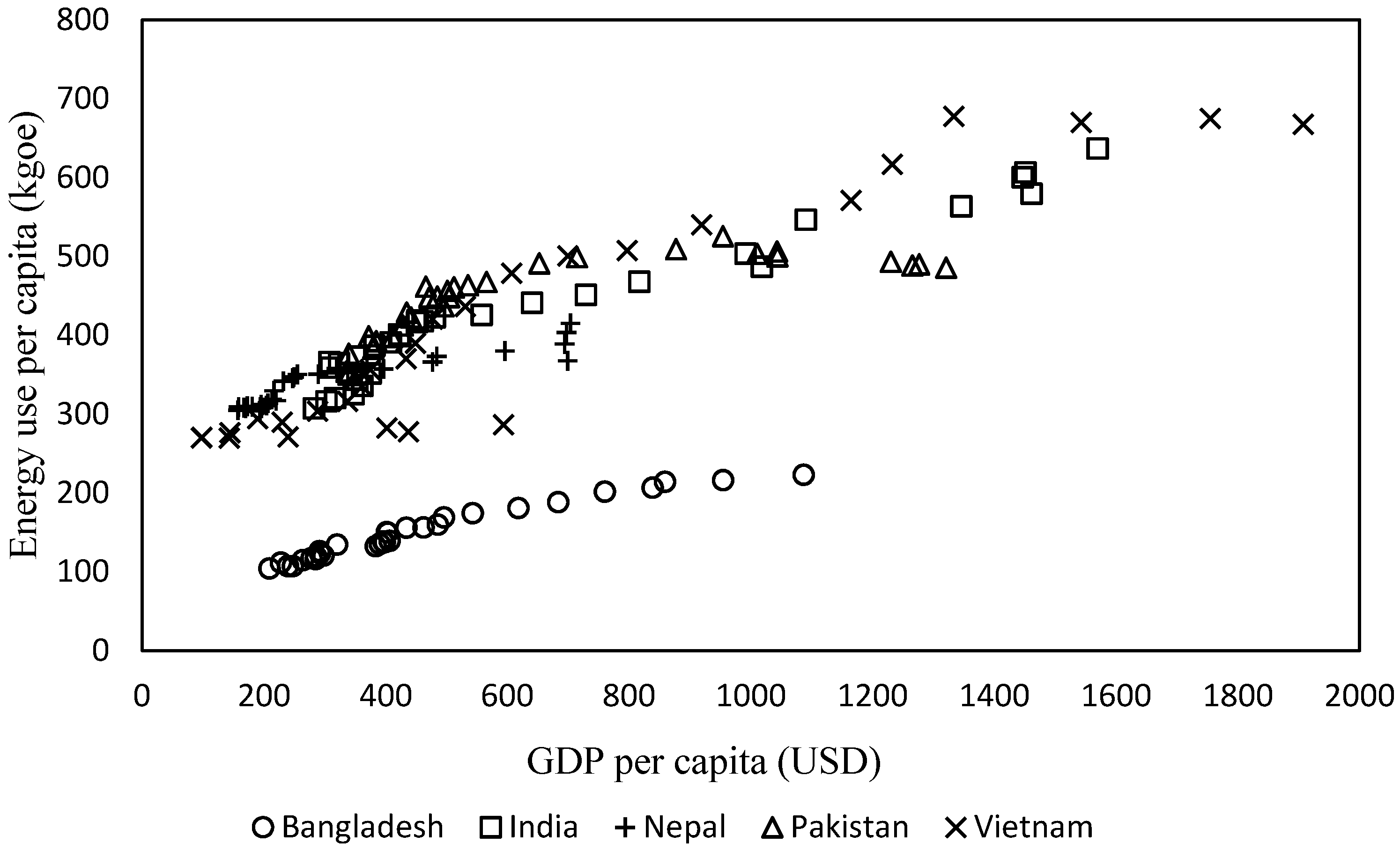
Average	354.47	677.67	103.91	137.07	539.03	1907.56	97.16	370.89

shows the summary statistics of countries that belong to the low-income group, consisting of countries whose average GDP per capita during 1984–2014 is under 1000 USD. As seen in the table, all the countries in this income group have energy consumption per capita under 1000 kgoe. This indicates that these countries not only have a low level of GDP per capita but also have small energy consumption per capita compared to other Asia-Pacific countries. Figure 2 is the plots of GDP and energy consumption per capita for these low-income group countries. It is apparent from the figure that most of the energy consumption per capita for these countries tends to increase as their GDP per capita grows.

Table 3. Summary statistics of energy consumption (kgoe) and GDP (USD) per capita for middle-income group.

Country	Energy Use Per Capita (Kgoe)				GDP Per Capita (USD)
	Mean	Max	Min.	Std. Dev.	Mean	Max	Min.	Std. Dev.
China	1167.23	2236.73	651.08	531.60	1885.61	7683.50	250.71	2195.06
Indonesia	676.87	886.26	393.51	155.37	1366.61	3700.52	442.15	1072.27
Mongolia	1368.97	1847.10	944.39	309.22	1458.34	4400.62	339.52	1229.58
Philippines	459.48	513.14	416.69	25.74	1255.91	2873.09	535.24	681.05
Sri Lanka	404.63	551.02	315.56	73.34	1265.11	3852.74	377.64	1048.66
Thailand	1184.65	2012.06	446.39	469.07	2788.91	6225.05	747.49	1622.96
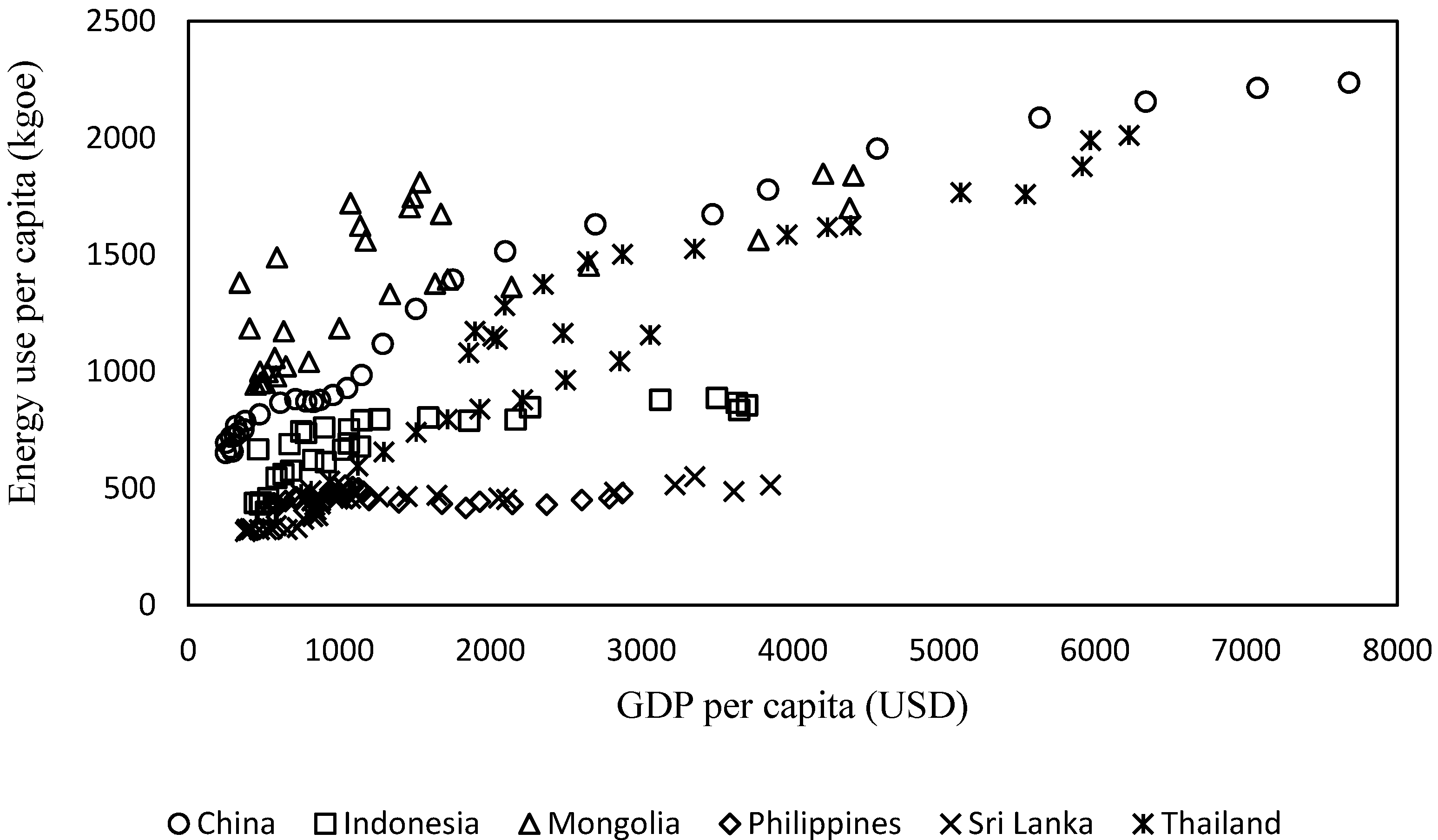
Average	874.31	2236.73	315.56	495.22	1671.23	7683.50	250.71	1481.15

illustrates the summary statistics of the middle-income group, which contains countries with an average GDP per capita above 1000 USD and below 3000 USD. As seen in the table, six countries are categorized into this income group. None of these countries have energy consumption per capita above 3000 kgoe and the group average energy consumption per capita level is way below the average of the 19 Asia-Pacific countries (2088 kgoe). From Figure 3, similar to the case of the low-income group, it is apparent that most of these countries have an upward trend in their energy consumption per capita as their GDP per capita increases.

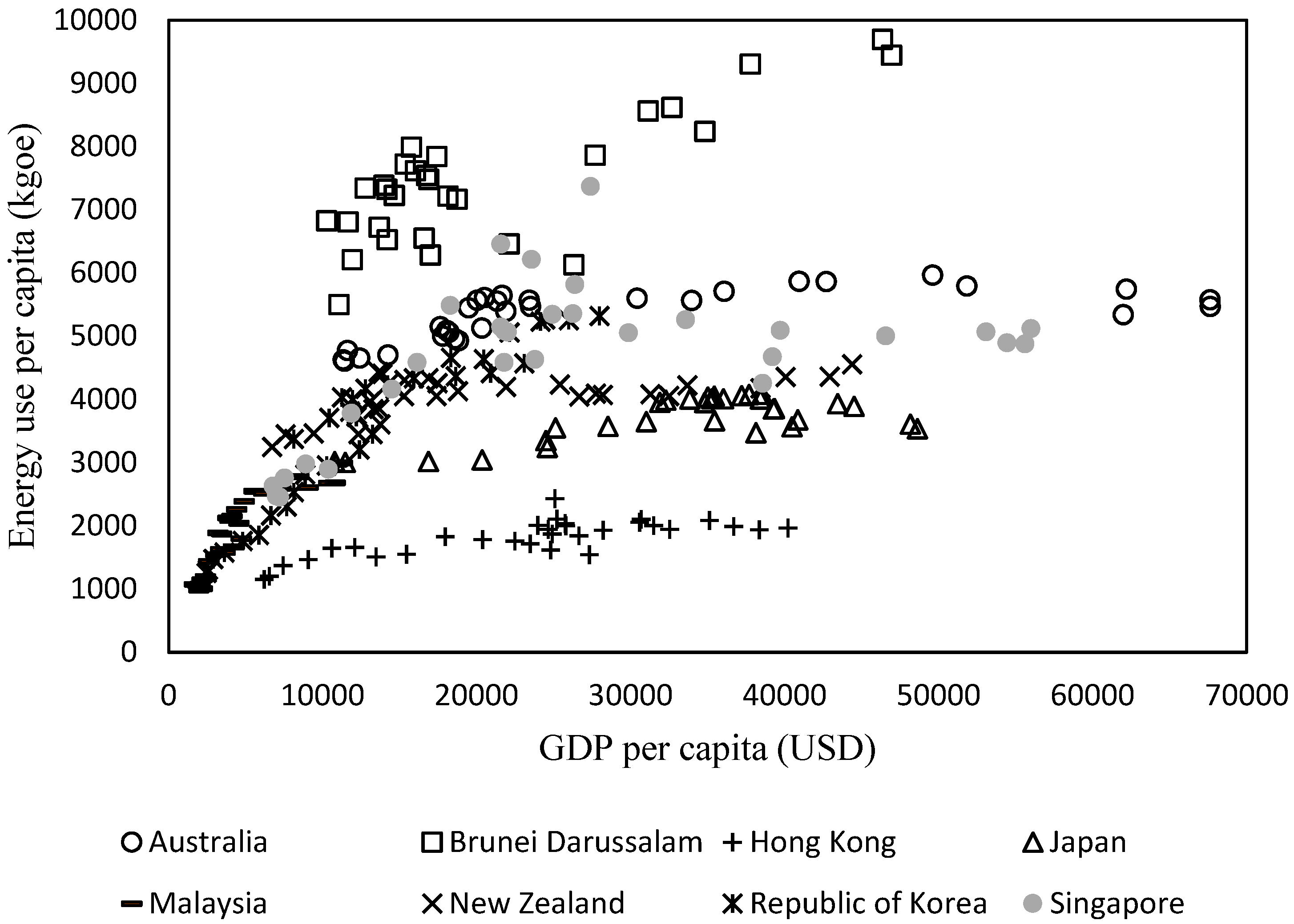
Finally,

Table 4. Summary statistics of energy consumption (kgoe) and GDP (USD) per capita for high-income group.

Country	Energy Use Per Capita (Kgoe)				GDP Per Capita (USD)
	Mean	Max	Min.	Std. Dev.	Mean	Max	Min.	Std. Dev.
Australia	5336.05	5964.67	4602.96	403.93	29,284.55	67,652.68	11,361.27	17,500.22
Brunei	7466.88	9695.71	5499.11	1003.36	22,211.28	46,973.94	10,280.77	11,333.64
Hong Kong	1811.16	2431.88	1156.80	284.20	23,340.14	40,215.49	6208.23	9452.82
Japan	3703.11	4083.83	3005.24	352.05	33,485.16	48,629.20	10,786.79	9440.74
Malaysia	1972.63	2999.90	986.29	646.31	5043.63	11,305.90	1709.71	2962.66
New Zealand	4034.92	4559.89	3251.01	324.42	20,986.47	44,380.43	6713.60	10,774.30
Rep. of Korea	3518.57	5323.13	1257.12	1304.35	13,310.29	27,989.35	2474.47	7530.92
Singapore	4665.71	7370.65	2455.48	1188.68	26,338.81	56,007.29	6793.55	15,151.50
Average	4063.63	9695.71	986.29	1884.22	21,750.04	67,652.68	1709.71	13,994.68

depicts the summary statistics for the high-income group whose average GDP per capita is above 5000 USD during 1984–2014. As seen in the table, there are eight counties in this income group. All these countries consume energy above the average energy consumption of the whole Asia-Pacific region and have a GDP per capita above 10,000 USD at some point. Figure 4 illustrates the data of countries belonging to this income group. The figure tells us that except for Brunei and Malaysia, all the countries in this income group have a turning point for their energy consumption per capita. We believe the reason for Brunei and Malaysia not having a turning point in the figure is because these countries are petroleum-exporting countries and economic growth of these countries depend largely on petroleum.

4. Results

The specification tests performed to select the most statistically appropriate model for the panel regression model for the whole sample suggest that the fixed-effects model fits the best. The results of the Wald test in

Table 5. Specification tests for the panel regression model.

	Wald Test		LM Test			Hausman Test
Test Statistics	F-Stat.	Chi-Square	BP Test	Honda	King-Wu	Chi-Square
Whole sample	311.11 ***	5599.97 ***	5674.20 ***	75.33 ***	75.33 ***	22.84 ***
Low-income group	674.04 ***	2696.15 ***	1820.55 ***	42.67 ***	42.67 ***	1.30
Middle-income group	223.81 ***	1119.07 ***	1789.77 ***	42.31 ***	42.31 ***	1.49
High-income group	460.18 ***	3221.24 ***	3199.35 ***	56.56 ***	56.56 ***	0.08

Note: *** indicates significant at the 1% level.

indicate that the fixed-effects model is preferred to the pooled-OLS model. The LM test implies that the random-effects model is more applicable compared to the pooled-OLS model. Finally, the Hausman test detects that the fixed-effects model is preferred to the random-effects model.

Hence, we used the fixed-effects model for testing the EEKC hypothesis for the whole sample and the random-effects model for the low-, middle-, and high-income groups.

Table 6. Estimation results for panel regression models.

	FE Model	RE Model
	Whole Sample	Low-Income	Middle-Income	High-Income
Intercept	3.81 ***	5.64 ***	6.79 ***	−9.14 ***
Ln (GDP)	0.53 ***	−0.28	−0.37	3.28 ***
(Ln (GDP))2	−0.01 ***	0.05 ***	0.05 **	−0.15 ***

Note: FE and RE represent fixed-effects and random-effects. *** and ** indicate. significant at the 1% and 5% levels.

shows the results of the panel regression estimation. From Table 6, it can be seen that the fixed-effects model for the whole Asia-Pacific sample satisfies all the conditions of the EEKC hypothesis. This result implies that there is a turning point among the 19 Asia-Pacific countries where the energy consumption per capita starts to decrease as GDP per capita exceeds a certain level. However, calculating the GDP per capita at its turning point for the whole Asia-Pacific region using the results of Table 6, it turned out to be about 98.1 million USD. This value is unrealistic for a GDP per capita. Similarly, the model for the high-income group indicated that the EEKC hypothesis holds among the countries with an average GDP per capita above 5000 USD. The GDP per capita at the turning point of this model was about 44,572 USD. This value is still higher than the average GDP of the high-income group, but it is a more realistic value compared to the one obtained for the whole sample model.

On the other hand, according to Table 5, the random-effects model is the best fit model for the low-, middle-, and high-income groups. For all these income groups, the Wald and LM tests point to either the fixed- or the random-effects model as the suitable model. Then, the Hausman test demonstrates that the random-effects model is preferred to the fixed-effects model.

On the other hand, the models for the low- and middle-income groups did not meet the EEKC hypothesis because the coefficients for the GDP were not significant and those for the squared-GDP were positive. As seen in Figure 2 and Figure 3, this is perhaps because most of the energy consumption of countries belonging to the low- and middle-income groups had an upward trend as their GDP grew.

Next, we will explain the results of the panel cointegration model.

Table 7. Panel unit root tests.

Whole sample
	Level			First difference
	LLC	Breitung	IPS	LLC	Breitung	IPS
Energy	−0.98	4.17	2.61	−13.93 ***	−6.98 ***	−14.71 ***
GDP	−4.78 ***	0.66	−3.18 ***	−8.15 ***	−8.12 ***	−11.34 ***
Squared-GDP	−1.51 *	1.40	1.07	−8.54 ***	−8.29 ***	−11.16 ***
Low-income group
	Level			First difference
	LLC	Breitung	IPS	LLC	Breitung	IPS
Energy	−0.01	2.76	2.13	−8.27 ***	−6.27 ***	−9.52 ***
GDP	−4.59 ***	1.51	−4.04 ***	−2.39 ***	−3.80 ***	−6.86 ***
Squared-GDP	0.65	2.18	1.07	−2.24 **	−4.04 ***	−6.48 ***
Middle-income group
	Level			First difference
	LLC	Breitung	IPS	LLC	Breitung	IPS
Energy	−0.43	1.62	2.13	−4.91 ***	−3.69 ***	−6.01 ***
GDP	−0.84	1.54	0.70	−5.06 ***	−5.10 ***	−6.44 ***
Squared-GDP	−0.49	2.40	1.57	−5.58 ***	−4.97 ***	−6.35 ***
High-income group
	Level			First difference
	LLC	Breitung	IPS	LLC	Breitung	IPS
Energy	−1.16	3.07	1.22	−11.07 ***	−3.57 ***	−9.95 ***
GDP	−2.58 ***	−0.62	−2.28 ***	−6.42 ***	−5.13 ***	−6.45 ***
Squared-GDP	−2.55 ***	−0.66	−2.00 **	−6.64 ***	−5.26 ***	−6.56 ***

Note: The test includes both intercept and linear trend. ***, **, and * indicate significant at the 1%, 5%, and 10% levels, respectively.

and

Table 8. Panel cointegration tests.

	Whole Sample	Low-Income	Middle-Income	High-Income
Pedroni test	Test statistics	Test statistics	Test statistics	Test statistics
Panel v-Statistic	2.05 **	7.25 ***	1.96 **	−0.38
Panel rho-Statistic	0.94	−0.82	0.56	−0.36
Panel PP-Statistic	−1.87 **	−1.97 **	0.05	−2.54 ***
Panel ADF-Statistic	−3.46 ***	−1.92 **	−0.38	−3.05 ***
Group rho-Statistic	2.02	−0.36	1.41	1.54
Group PP-Statistic	−3.91 ***	−2.69 ***	0.53	−2.41 ***
Group ADF-Statistic	−2.35 ***	−2.69 ***	−0.59	−0.99
Kao test	Test statistics	Test statistics	Test statistics	Test statistics
t-statistic	−3.12 ***	−1.68 **	−1.62 *	−4.24 ***

Note: The test includes both intercept and linear trend. ***, **, and * indicate significant at the 1%, 5%, and 10% levels, respectively.

show the precondition test results of the cointegration model. Table 7 illustrates the results of the stationarity tests performed on all variables investigated in this study. From the table, the Breitung test suggests that all the test variables are integrated at order one, which means that at least at some levels, all the variables are stationary when first differencing them.

From Table 8, we can see that the majority of the Pedroni test statistics indicate that the null hypothesis of no cointegration is rejected for the whole sample and low-income models. The Kao test also reveals that the test variables are cointegrated in these models. Therefore, we conclude that the whole sample and low-income models strongly satisfy the preconditions of the cointegration model estimation. On the contrary, the results for the middle-income model in the table imply that the test variables are not cointegrated and the Kao test can only reject the null hypothesis of no cointegration at the 10% significance level. Thus, it is likely that the variables for the middle-income model are not cointegrated. Finally, the Pedroni test for the high-income model also did not provide strong evidence of having a cointegrating relationship among the test variables. However, we conclude that the variables in the high-income model are weakly cointegrated because at least the three test statistics in the Pedroni and Kao tests indicate evidence of cointegration.

Hence, we determined that the preconditions for the cointegration test were met except for the middle-income group model. Following this result, we estimated the FMOLS and DOLS models for the whole sample, low-, and high-income groups.

Table 9. Estimation results for the FMOLS and DMOLS models.

	Whole Sample		Low-Income		High-Income
	FMOLS	DOLS	FMOLS	DOLS	FMOLS	DOLS
Ln (GDP)	1.87 ***	1.79 ***	0.042	0.0887	3.66 ***	3.52 ***
(Ln (GDP))2	−0.09 ***	−0.09 ***	0.008	0.0035	−0.19 ***	−0.18 ***

Note: The test includes both intercept and linear trend. *** indicates significant at the 1% level.

presents the results of the panel cointegration model for the whole sample, low-, and high-income groups. From the table, it is evident that the coefficients of whole sample and high-income group models satisfy the condition of the EEKC hypothesis. This is consistent with the estimation of the panel regression model, which tells us that it is conceivable that the EEKC hypothesis does hold for the whole sample and high-income group. As the whole sample and high-income group models meet the EEKC hypothesis, we also estimated the GDP per capita at their turning points. The estimated GDP per capita at the turning points of the FMOLS and DOLS models for the whole sample were 20,169 and 17,336 USD, respectively. Those for the high-income group turned out to be 19,537 and 19,456 USD, respectively.

It is noticeable from Table 4 that the estimated GDP per capita at the turning point for the high-income group model is less than its average GDP per capita (21,750 USD). This might be implying that the high-income group in the Asia-Pacific countries is already achieving an economic growth beyond the income level to satisfy the win–win situation (economic growth with decreasing energy consumption) of the EEKC hypothesis.

5. Discussions and Conclusions

Understanding the transition in the relationship between energy consumption and economic growth for Asia is crucial because now Asia is the world’s largest energy-consuming region and it is also becoming the largest contributor to greenhouse gases. Hence, to understand the energy-consumption and economic-growth relationship, we investigated the EEKC hypothesis among the 19 Asia-Pacific countries for the 1984–2014 period. Both the panel regression and cointegration models indicated that the EEKC hypothesis persists among the Asia-Pacific countries. However, the test performed on low-, middle-, and high-income groups in the Asia-Pacific region suggested that the EEKC hypothesis only stands for the high-income group; the low- and middle-income groups did not meet the hypothesis. This might be implying that although there exists a turning point where the energy consumption per capita starts to decline as the Asia-Pacific countries achieve economic development, such a transition in the energy consumption is only occurring in the developed countries. It could be that countries that are struggling with poverty have no room to implement an energy policy to increase their energy efficiency. It is probable that for such countries, economic development is their higher priority than introducing more efficient energy sources to mitigate environmental pressure.

However, our results also suggested that once the countries move to the high-income group (average GDP per capita above 5000 USD), there is a chance that a country can develop along the EEKC path and achieve economic development without adding environmental pressure. Hence, this indicates the importance of developed countries in the Asia-Pacific region to provide economic and technological support for the developing countries in the region to catch up with them.

Although the panel regression estimation did not provide us with a realistic GDP per capita at the turning point of the EEKC for the whole Asia-Pacific sample, the DOLS cointegration model provided us with a potentially achievable level of GDP per capita. This result implied that the panel cointegration model prevails against the panel regression model for analyzing the EEKC.

According to the estimation of the DOLS model, once the GDP per capita of the Asia-Pacific country exceeds 17,336 USD, the country starts to develop along the EEKC path. One might argue that this estimated income per capita is still high compared to the current average GDP per capita of the Asia-Pacific region. However, our DOLS model also found that the GDP per capita at the turning point of the EEKC for the high-income group was 19,456 USD. This income value was less than the average GDP per capita among the high-income group during 1984–2014. This might be indicating that the developed countries in the Asia-Pacific region are already achieving economic growth along the EEKC.

All in all, although this study suggests that the EEKC hypothesis stands for the Asia-Pacific region, it is likely that the transition in the energy consumption along the line with the EEKC is only taking place in the developed countries. As countries with an average GDP per capita below 3000 USD did not meet the EEKC hypothesis but rather had an upward trend in the energy consumption as their income grew, a rigid energy policy is required for these developing countries to reduce their energy consumption. However, we believe this is not a difficult task for the Asia-Pacific region because our study shows that at least the developed countries of the region are already growing with decreasing energy consumption. It is probable that there is a chance for these developing countries to learn and make use of energy policies that worked effectively in these developed countries and work together with the developed countries to achieve such sustainable development.

For further study, we need to find out what policy would be effective and what support the developed countries could provide for the developing countries to achieve economic development along the EEKC. As this was the first study to test the EEKC hypothesis for the Asia-Pacific region, our model was kept in a simple form, having only income and its quadratic form as dependent variables. However, we should further pursue the research with other variables that might be meaningful to be included in the EEKC model such as income disparity, access to electricity, average electricity price, and so on.