Article

Learning Curve Analysis of Wind Power and Photovoltaics Technology in US: Cost Reduction and the Importance of Research, Development and Demonstration

Institute of Energy, Environment and Economy, Tsinghua University, Beijing 100084, China
*
Author to whom correspondence should be addressed.
Sustainability 2019, 11(8), 2310; https://doi.org/10.3390/su11082310
Submission received: 11 March 2019 / Revised: 12 April 2019 / Accepted: 15 April 2019 / Published: 17 April 2019

Abstract

:
The strategic transition from fossil energy to renewable energy is an irreversible global trend, but the pace of renewable energy deployment and the path of cost reduction are uncertain. In this paper, a two-factor learning-curve model of wind power and photovoltaics (PV) was established based on the latest empirical data from the United States, and the paths of cost reduction and corresponding social impacts were explored through scenario analysis. The results demonstrate that both of the technologies are undergoing a period of rapid development, with the learning-by-searching ratio (LSR) being greatly improved in comparison with the previous literature. Research, development, and demonstration (RD&D) have contributed to investment cost reduction in the past decade, and the cost difference between high and low RD&D spending scenarios is predicted to be 5.5%, 8.9%, and 11.27% for wind power, utility-scale PV, and residential PV, respectively, in 2030. Although higher RD&D requires more capital, it can effectively promote cost reduction, reduce the total social cost of deploying renewable energy, and reduce the abatement carbon price that is needed to promote deployment. RD&D and the institutional support behind it are of great importance in allowing renewables to penetrate the commercial market and contribute to long-term social welfare.

1. Introduction

Energy crises have become increasingly prominent worldwide. At the end of 2017, it was estimated that the known reserves of oil, natural gas, and coal will only be able to meet energy requirements for 50.2, 52.6, and 134 years, respectively, according to the 2017 annual production level. However, the high demand for economic growth and energy consumption continue, as exemplified by the 1.7% average growth rate in the global primary energy consumption from 2006 to 2016 [1]. This contradiction necessitates a strategic transition from energy production via fossil fuels to the use of renewable energy sources. Countries and organizations, such as China [2] and European Union (EU) [3], have proposed specific targets in energy transition. However, the fulfilling of targets proved to be difficult [4,5]. In order to achieve the energy transition, effective policy instruments and their economic impacts need to be carefully studied [6]. Among the renewable technologies, wind power and photovoltaic (PV), as clean, high-efficiency, and convenient methods of energy production, are playing increasingly significant roles in the global energy structure transition. In 2010–2017, the annual global incremental investments in PV and wind power were over $200 billion [7]. By the end of 2017, the global cumulative installed capacities of wind power and PV had reached 514 and 390 GW, and the power that was generated from these sources represented 5.6% and 1.9% of the total, respectively [8]. Thus, the laws governing the development of wind power and PV, and their relationship with policy, are of particular importance.
The Obama administration was active in global climate governance. They attached importance to the strategic transition of the energy structure, and vigorously promoted the development of clean-energy technologies [9,10]. In 2008–2016, American research, development, and demonstration (RD&D) spending for wind power and PV combined was over $2 billion [11]. With this strong policy support, the United States achieved much in energy transition. In the same period, energy-related carbon dioxide emissions and carbon intensity reduced by 11% and 22%, respectively. The share of coal in total electricity generation dropped from 49% to nearly 31%, which was mainly due to replacement by gas-fired power and renewables [12]. In 2016, the cumulative installed capacities of wind power and PV reached 82 and 33 GW, respectively, with electricity shares of 5.3% and 1.1% [8]. However, in 2016, the Trump administration issued the “America First Energy Plan”, and the executive order on energy independence promoting traditional American energy industries and investigated the laws and regulations from the Obama era, especially the “Clean Power Plan”. Subsequently, on 1 June 2017, the Trump administration announced the withdrawal of the United States from the Paris Agreement, and the 2018 annual-budget proposal illustrated that all of the energy-related research projects, especially those involving renewables, would face budgetary constraints [13]. In the United States (US), wind power and PV continue to compete with gas-fired power, which is still advantageous in terms of cost. Thus, cost reduction is the key to the further penetration of renewables. Policy makers, investors, and society have highly considered the cost reduction path and its social impacts.
The learning curve is an effective way of looking at energy cost reductions. It is based on the basic assumption that experience, knowledge, and other factors can improve technology performance, depicting the trend that the unit cost declines with the accumulation of factors above. The modeling method is the fitting of each factor and unit cost. The sample period of the existing literature is concentrated before 2010 [14,15,16,17,18,19,20,21]. Therefore, the rapid expansion of installed capacity and the rapid decline of investment costs in recent years have not been taken into account, and the estimation of model parameters needs to be updated. In addition, most discussions regarding the results have focused on the reasons for structural changes in the model parameters, such as learning rates and time lag, and there has been little judgment on the social impacts that are caused by the cost-decline path under the learning-curve rule. This article establishes a two-factor learning-curve model about US PV and wind power that is based on the most recent empirical data and explores the cost-reduction contribution of cumulative production and knowledge stock. On the basis of the learning rates, the article then analyzes the influence of changes in installed capacity development and RD&D spending on wind power and PV cost reduction from 2017 to 2030, as well as the resulting changes in investments, social costs, carbon abatement, and abatement carbon price. Figure 1 shows the structure of this paper:

2. Literature Review

2.1. Learning-Curve and Variable Selection

Wright conducted the first empirical study on the learning curve in aircraft manufacturing in 1936 [22], and the Boston Consulting Group introduced this concept into relevant studies in management science in 1968 [23]. Researchers have put forward various types of learning mechanisms, mainly including learning-by-doing, learning-by-searching, and learning-by-using. These models are classified into four categories that are based on the number of included factors: one-factor, two-factor, three-factor, and multifactor models. Table 1 summarizes the different learning-curve models.
The one-factor learning curve only reflects the learning-by-doing mechanism. The unit cost decreases from the initial position with an increase in cumulative production. Its decreasing speed is illustrated by the elasticity coefficient a. The learning rate is defined as 1–2-a, which denotes the percentage change in cost as a consequence of doubling the cumulative production. The one-factor learning curve reached its highest popularity in the mid-1970s. Companies were encouraged to expand production to block the entrance of competitors and gain long-term cost advantages [25]. With further study, some researchers realized that the one-factor learning curve only considers the effects of technology from the demand side and, in certain cases, is very sensitive to the choice of data and variables [26]. Thus, they discomposed the learning effects into learning-by-doing and learning-by-searching, that is, a two-factor model. Average scale Q is further included by the three-factor model. The learning-curve model with three factors and above often has the problem of collinearity [24]. Therefore, in empirical studies, one-factor and two-factor models are most frequently used.
When the elasticity coefficient stays constant, the unit cost decreases at a certain rate with cumulative production. In practice, the learning speed of energy technology has been evolving. Therefore, researchers incorporate the path of dynamic changes in the learning curve of energy technologies. Yelle [27] identified models that illustrate the dynamic law, including the S-model, Plateau model, and Stanford-B model. In practice, most studies divide the cost-reduction process into multiple stages [24,28,29], which is, in essence, the combination of multiple static curves at different time ranges. Therefore, the multistage dynamic learning curve can be supplemented when the static curve cannot be well-fitted.
In research, different indicators can depict the unit cost, cumulative production, and knowledge stock in energy technologies. For example, the depiction of the unit cost of renewables usually involves the price of components [18,30,31], the costs of power generation [32,33,34], investment costs [14,19,20], and the trading prices of electricity [35]. Financial discounts affect the power generation costs. Prices of power purchase agreements are affected by several uncertain factors, including the supply–demand relationship and government subsidiaries. Therefore, the unit-investment cost ($/Kw) is considered to be the most accurate indicator for endogenous energy technology learning processes [36].
Around the year 2000, the researchers noticed that the impact of historic RD&D investments in current technology had declined over time [37]. For such investments to exert substantial impacts on technology development and cost reduction also takes time. Thus, researchers developed the recursion of knowledge stock. Assuming the decay factor and the time lag years, the knowledge stock for a certain energy-technology is as follows [38,39]:
K S t + 1 = K S t × ( 1 ρ ) + R D D t + 1 g
ρ = decay factor; g = time lag (year); K S t = knowledge stock in year t.
The learning-curve approach has some limitations. In fact, the cost of energy technology could rise in some sample years, such as the global weighted-average installation cost of wind power from 2004 to 2009 [40]. Some studies also showed negative-learning rates [41,42]. These show that the decrease in the unit cost with the increase of cumulative production at a specific learning efficiency is a phenomenon that is based on empirical observation rather than an inevitable endogenous rule. However, it is still of great significance in the understanding of changes in energy-technology cost and the improvement of the integrated model of energy economic environments.

2.2. Studies on the Learning Curve of US Wind Power and Photovoltaics
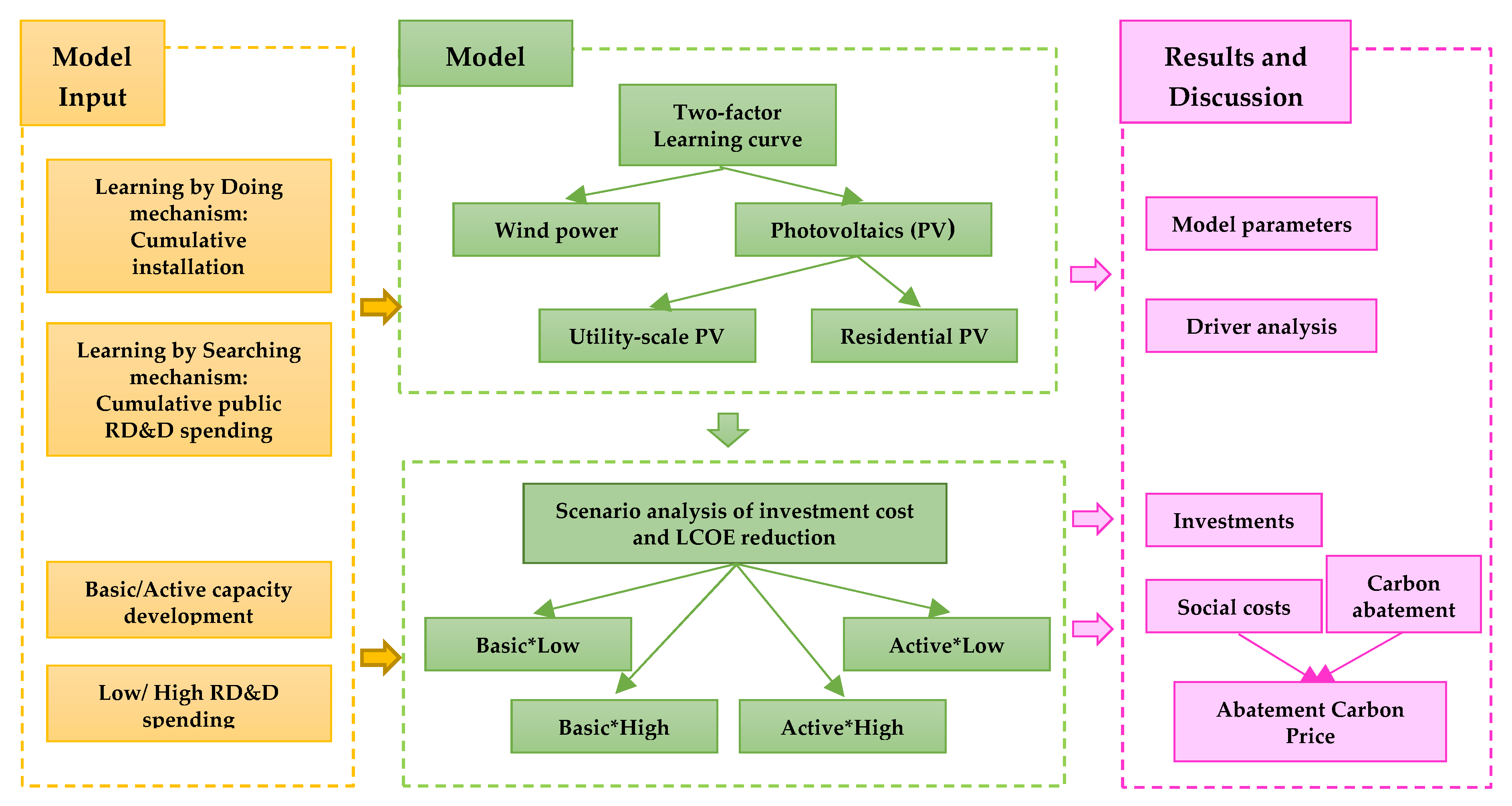
The United States developed a strong interest in wind-power and PV generation after the first oil crisis in 1973. In 1974, the US Congress approved the “Solar Energy Research Act” to authorize a vigorous solar-energy research program [43]. In the early 1980s, the first grid-connected wind turbine was installed in the United States. At that stage, the research, development, and commercialization of solar and wind began to bloom, and so did learning curve studies regarding them. The existing literature on the learning curve of wind power and PV in the United States has mostly adopted the single-factor model, while some studies also used two- and three-factor models. The learning-by-doing ratio (LDR) for wind power is typically about 16–32% in the single-factor model [14,15,16,18,19] and 12–14% [20,21] in the two-factor models, while the two-factor model learning-by-searching ratio (LSR) is typically about 16–18%. The LDR is 16–32% in the single-factor PV models [17,29], around 18% in two-factor models [20,21], and the corresponding LSR is 12–15%. The learning rates of American’s wind power and PV have been over 10% since the 1980s, indicating evolving they are technologies according to Jamasb’s classification [26].

3. Methods

3.1. Learning-Curve and Variable Selection

When considering all of the factors that are introduced above, a two-factor learning curve was adopted in this study. The unit cost is depicted by unit investment costs, cumulative production is represented by the cumulative installed capacity, and knowledge stock is represented by cumulative effective RD&D spending. RD&D spending covers all of the energy-related fundamental research, application research, and demonstration projects, but it excludes relevant administrative and education expenses [44]. Public RD&D spending was used for two reasons: (1) calculation of nongovernmental spending is challenging and (2) it can more directly reflect the impact of policy changes.
The introduction of a time lag and decay factor in learning curves can lead to high statistical flexibility and a good fit for the data. Endogenously different reactions to RD&D spending among different industries can also be better explained. Therefore, this study also used Equation (1), while changing the (g,ρ) value into different combinations. Subsequently, the independent variables and dependent variable were linearly fitted with Statistical Package for the Social Sciences (SPSS) statistical software. For linear fitting, the Ordinary Least-Squares (OLS) method was adopted, which searches for the best match by minimizing the sum of squared errors. OLS applications have a set of assumptions that require the consideration of autocorrelation, nonnormality, and multicollinearity. Therefore, in this paper, the goodness-of-fit test, T test, Durbin-Watson (DW) test, and multicollinearity test were performed on the fitting results, and acceptable significance was set to be less than 10% to ensure that the error term was independent, there was no sequence correlation, and that the explanatory variables were linearly independent. Of all the models that passed the tests, the one with the best fitting was selected. All of the economic data used for this article were below the 2016 constant price. Table 2 provides the sources of the selected data.
The learning rates, LDR and LSR, are the percentage of cost reduction when the production or RD&D spending doubles, indicating the cost-reduction speed in this period. In reality, the two factors grow and double differently, and the learning rates are not equal to the contribution of two factors. Thus, this paper uses the following method to calculate the contribution of different factors. Cost reduction in year t when compared to the costs in 2009 can be divided into the cumulative production part Δ C t C C and the cumulative RD&D spending part Δ C t K S . They are calculated, as follows:
Δ C t C C = C o × ( C C t a C C 2009 a ) × K S 2009 b
Δ C t K S = C o × ( K S t b K S 2009 b ) × C C 2009 a .
where C C t and K S t are the values of cumulative production and cumulative RD&D spending in year t, and C C 2009 and K S 2009 are the values in 2009. a and b are the elasticity coefficients of cumulative production and cumulative RD&D spending. Further, the contribution of cumulative installation capacity P c c and the contribution of effective cumulative RD&D spending P K S are:
P c c = Δ C t C C Δ C t C C + Δ C t K S
P K S = Δ C t K S Δ C t C C + Δ C t K S

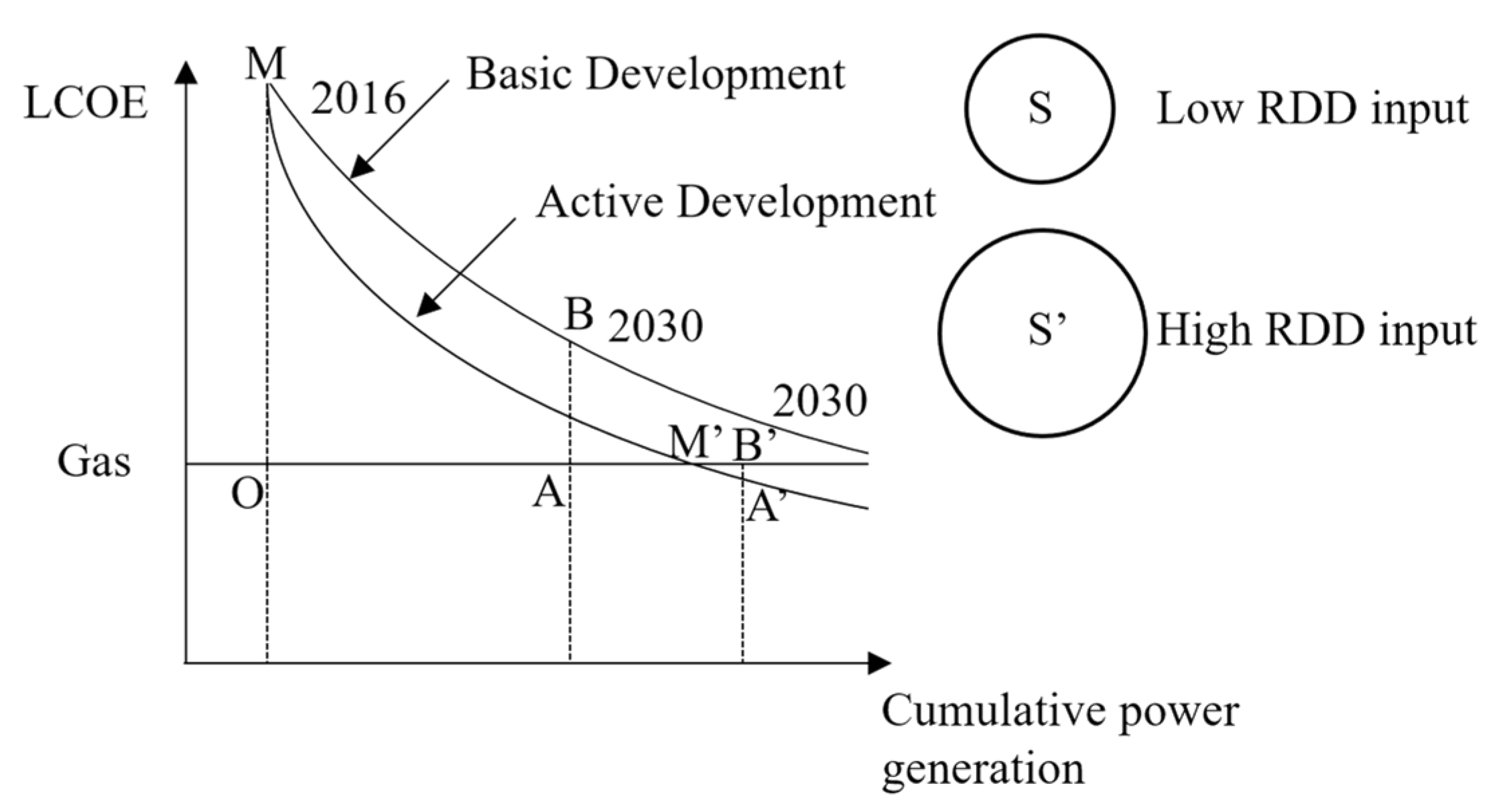
3.2. Scenario Settings

Four scenarios were considered to predict the future situation: two capacity-development scenarios, basic and active, and two RD&D spending scenarios, high and low. In the report of the US Energy Information Administration (EIA) “Annual Energy Outlook 2018” [47], it is stated that, under the reference scenario, namely, the law of economic and demographic changes and other laws and regulations do not change, and the installed wind capacity will reach 131 GW by 2030. A less conservative view is that it could reach 200 GW with optimistic technological innovation and cost reduction [48]. The learning-curve model assumes that production happens before cost reduction. Therefore, with reference to other studies, this paper set the accumulative installed capacity for 2030 as 130 GW in the basic scenario and 200 GW in the active scenario. Installation would grow by 3.4 GW per year in the basic scenario and 8.4 GW under the active scenario, while assuming an even growth rate from 2017 to 2030. The assumption of PV mainly refers to IRENA’s prediction of a global installed capacity in 2030 of 1757 GW, of which 237 GW will be installed in the United States [49]. Cumulative PV installation in 2030 is predicted to be 150 GW in the basic scenario and 250 GW in the active scenario. The proportion of utility-scale PV is predicted to account for 70% of all PV installed, with residential PV representing 20%. This assumption is based on the fact that the proportion of utility-scale PV increased from 20% to 60% of all PV that were installed from 2010 to 2016, while residential PV basically remained at 20% after 2011. Installation is predicted to grow by 6.0 GW per year in the basic scenario, 11.1 GW in the active scenario, and 1.7 and 3.1 GW for residential PV, respectively.
When considering the two RD&D spending scenarios, the main reference is the historical average RD&D spending in the sample period. The average RD&D spending of wind from 2009 to 2017 was $93 million, so it was set at $113 million per year for the high-spending scenario and $73 million per year for the low-spending scenario. Due to the particularly high investment in PV in 2009, the historical average value of $120 million from 2010 to 2017 was used as the reference for PV, with an average spending from 2017 to 2030 of $100 million in the low-spending scenario, and $140 million in the high-spending scenario. Under such a setup, a total of $520 million more would be invested in the high-spending than the low-spending scenario for wind and PV, respectively.

3.3. Levelized Cost of Energy

The reduction of investment costs leads to levelized cost of energy (LCOE) reduction. LCOE is the total present value of the cost, divided by the total present value of electricity generation over the life cycle of the project, which is suited to the comparison of different energy technologies [50,51]. The simplified LCOE algorithm is referred to in this paper, and the calculation equation is as follows [52,53]:
L C O E = C t + n = 1 N A n ( 1 + r ) n n = 1 N E n ( 1 + r ) n
where C t is the unit investment cost in year t, also the initial unit investment cost of the project. A n is the fixed operating cost in year n, including personnel costs and maintenance costs. Since wind and photovoltaic power come from free sources, fuel costs are not included. E n is the generated power in year n. As this paper considers unit values, E n is numerically equal to the power generated from a unit-power plant operating, in accordance with the capacity factor for a full year.   r is the discount rate, which reflects the judgment of stakeholders on the time value of the capital. In this paper, the payback period of assets was set as 20 years under benchmark conditions and a discount factor of r = 7.5%, in accordance with IRENA [40].
According to the Electric Power Monthly data from EIA [54], from 2013 to 2017, the wind power capacity factor ranged from 32.2% to 34.6%, and that of utility-scale PV ranged from 25.1% to 25.9%. When considering that the wind power capacity factor has seen a growth trend in recent years, from 2017 to 2030, the predicted value of the wind power capacity factor is 36%, the utility-scale PV is 26%, and residential PV is slightly lower, at 19%. National Renewable Energy Laboratory’s (NREL’s) 2018 Annual Technology Baseline (ATB) [55] reported that the subsequent operating and maintenance (O&M) costs of wind energy, utility-scale PV, and residential PV will be 51, 14, and 24 $/kW/year, respectively. ATB’s wind-energy data seem relatively high when compared horizontally; thus, 28 $/kW/year, as reported by the 2016 Wind Technologies Market Report [56], was adopted in this article.

3.4. Social Costs and Carbon Abatement

The levelized energy cost reflects the cost over the whole life cycle, which covers the initial investment and subsequent operating and maintenance process. Wind power and PV compete with gas-fired power plants in their development process. If their LCOE is higher than that of gas-fired power plants, society actually pays additional costs for their deployment and grid access, including the government’s tax reduction and exemption and excess enterprise investment. In this paper, social cost is defined as the total additional cost that is paid by society throughout the process of high-cost wind-power and photovoltaic generation. It is the product of the LCOE cost difference between wind or PV and gas electricity, and the generated power, plus RD&D spending.
In year n, the LCOE of the project installed in year t is
L C O E ( t , n ) = C t + n = 1 N A n ( 1 + r ) n n = 1 N E n ( 1 + r ) n
C t = unit investment cost ($/KW) in year t; A n = fixed operating cost ($/KW) in year n; E n = generated power (KWh) in year n.
Only the new capacity in year t, that is, the difference between C C t and C C t 1 , is considered. Since utility-scale and residential PV share PV knowledge stock, the PV RD&D is only added to the social costs of the utility-scale PV calculation to prevent double counting. R D D n g is the RD&D spent, it is actually input in year n g , as there is time lag. The calculation equation of total social cost SC from 2017 to 2030 is as follows:
S C = n = 2017 n = 2030 [ t = 2017 t = n ( L C O E ( t , n ) LCOE g a s ) E n ( C C t C C t 1 ) + R D D n g ] .
Gas-fired plants are considered to be relatively mature, with a constant LCOEgas of $0.05/KWh [57]. Figure 2 is a schematic diagram of social costs under different paths. When compared with the basic scenario, the active scenario accelerates installation deployment, which increases cumulative installation, while investment costs decrease at faster rates. LCOE also drops faster while assuming the same levels of O&M, depreciation life, and capacity factor. The ratio of the total social costs for the basic scenario and the active scenario is OABM/(OMM’ − A’B’M’). The social cost of low and high RD&D spending is S:S’. The social costs vary among the four scenarios.
The deployment of wind power and PV not only brings social costs, but also carbon emission reduction. The social benefits can be calculated from the perspective of carbon abatement. Carbon emissions from gas-fired plants are calculated by using the emission factor of 500 g/KWh, as in this paper [58]. The break-even abatement carbon price P, which makes the social benefits of new capacity from 2017 to 2030 equal to the social costs, is calculated as in Equation (9). When the carbon price level is higher than P, the deployment of wind power will generate additional benefits rather than additional burdens.
P = S C n = 2017 n = 2030 [ t = 2017 t = n E n × ( C C t C C t 1 ) ]

4. Results and Discussion

4.1. Learning-Curve Evaluation of Cost Reduction

4.1.1. Wind Power

From 2009 to 2016, the compound growth rate of wind power installation in the United States was 12.91%. By the end of 2016, the total installed capacity had reached 82 GW and the annual electricity generation reached 229 TWh, which accounted for 5.31% of the total electricity generation [12]. Despite this rapid growth, it will still be difficult to reach the goal that was set by the Department of Energy (DOE) of generating 10% of electricity through wind power by 2020 and 20% by 2030 [59]. As shown in Table 3, the model obtained an LDR value of 17.53% for the cumulative installed capacity from 2009 to 2016, an LSR value of 37.13% for the cumulative effective RD&D spending, a time delay of four years, a decay factor of 0.025, and an adjusted goodness of fit (R2) of 0.981. The fitting results of the learning rates are affected by the inclusion of model factors and the selection of representational variables. The one-factor model does not take the contribution of RD&D into account, thus overestimating LDR, as shown in the research that is presented in Rubin [21]. Research regarding generation costs using one-factor models [15,18] also obtained different results from that of investment costs [14,16]. Kobos [20], as in this paper, adopted a two-factor curve using the cumulative installation capacity and the IEA’s RD&D data to study the situation in 1991–2000, obtaining an LDR of 14.2%, an LSR of 18.0%, a five-year time lag, and a 2.5% decay factor. The learning rates that were obtained in this paper were higher than his, with an LDR value even higher than that being achieved by some one-factor studies [14,16], indicating that, with large-scale investments and commercialization, the learning ability of wind power technology has substantially improved. The industry has moved into the stage that BCG defines as shakeout [23].
Figure 3 shows predictions under different scenarios. When compared with 2016, the investment cost of wind power is predicted to decrease by 19.6–30.8% by 2025 and 26.5–41.4% by 2030. In 2030, the maximum cost differences that are caused by installation and RD&D spending are predicted to be 132 and 118 $/KW, respectively, comprising about 12.60% and 11.27% of the total cost. The decrease in investment cost drives the decrease in LCOE. In 2030, the LCOE decline is predicted to be 25.5–37.4% lower than in 2016, and the lowest predicted LCOE is 0.0358 $/KWh.

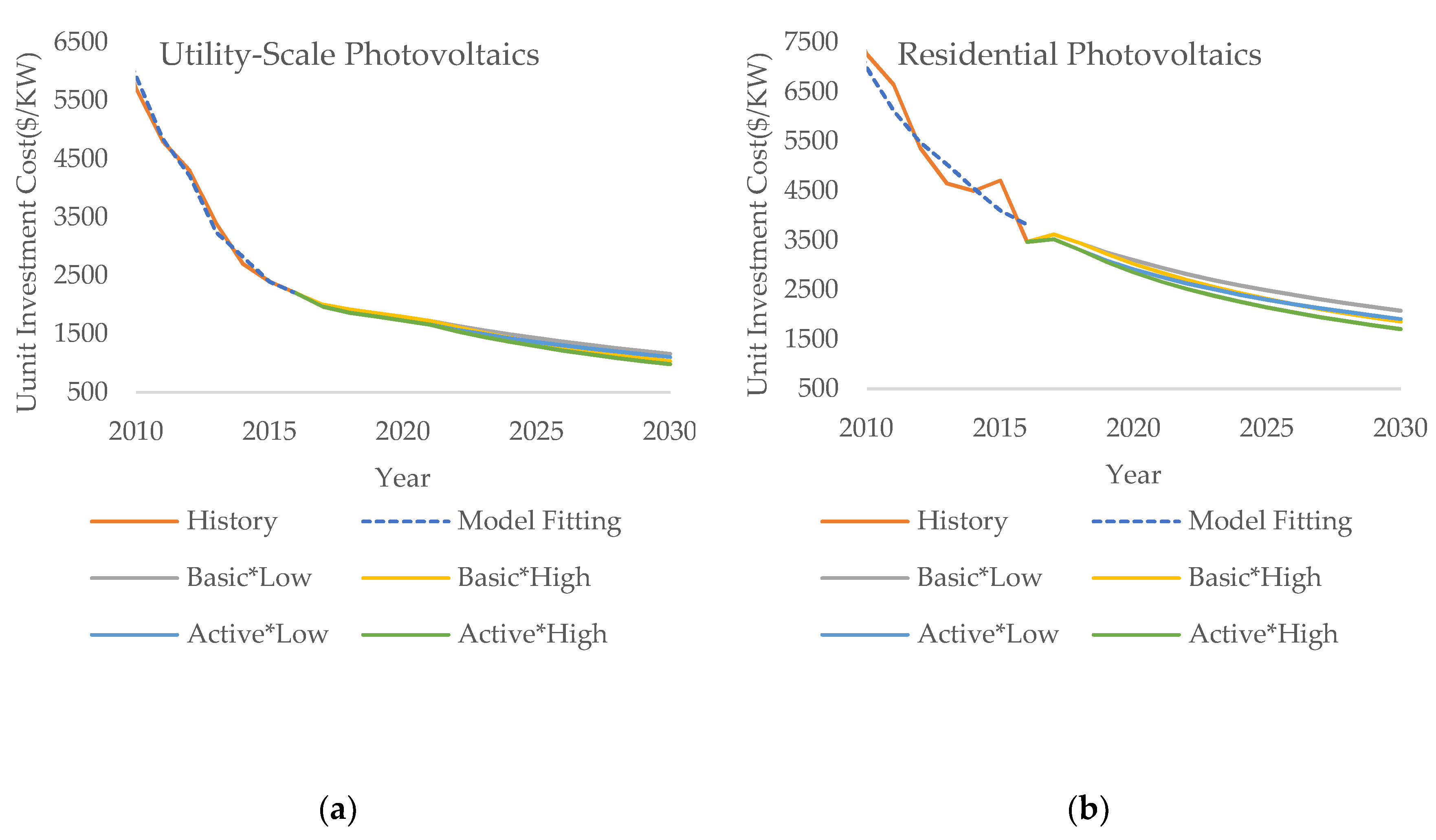
4.1.2. Photovoltaics

The installed capacity of PV has developed more rapidly, with a compound growth rate of 65.33% from 2009 to 2016. At the end of 2016, the total installed capacity of PV reached 33 GW and the annual power generation reached 46.6 TWh, which accounted for 1.08% of the total electricity generation [12]. PV systems can be divided into residential (0–10 KW), commercial (10–1000 KW), and utility-scale PV systems (>1000 KW) [40]. The installation share of utility-scale PV systems has constantly increased, from 20% in 2010 to over 60% by the end of 2016. In contrast, the share of commercial PV systems decreased over this period, and the share of residential systems stayed at almost 20% after 2012. In 2007, President Bush proposed a three-year solar program as part of his “Advanced Energy Initiative” [60] to accelerate the development of semiconductor materials and the improvement of system-level engineering. The Obama administration was also very supportive of clean-energy development. During their tenure, RD&D spending on solar-energy research significantly increased [11]. In 2010–2016, American utility-level PV investment costs were reduced by 61.42% and residential PV installation costs by 52.2% [45], reflected a significant cost reduction.
For utility-scale PV, in 2009–2016, the obtained LDR was 6.78% and the LSR was 75.21%, with a time delay of four years and a goodness of fit (R2) of 0.993. For the residential PV in 2007–2016, the obtained LDR was 10.86% and the LSR was 65.70%, with a time delay of one year and a goodness of fit (R2) of 0.949. PV LSR also became much higher. Kobos’s study [20] on US PV from 1988 to 2000 identified an LDR of 18.4%, an LSR of 14.3%, a time lag of three years, and a decay factor of 0.1. The PV LDR was lower than that of wind power and the LSR was higher, indicating that PV is at an earlier stage of the industrial cycle, and RD&D spending can more efficiently improve its technology, and thus reduce costs.
As shown in Figure 4, under the logic of the learning curve and scenario settings, the investment cost of utility-scale PV is predicted to decrease by 35.0–41.4% from 2016 to 2025 and by 47.1–55.3% to 2030. In 2030, the maximum cost differentials that are caused by installation and RD&D spending are predicted to be $127 and $59 per KW, respectively, or about 11.8% and 5.5% of the total cost. The investment cost of residential PV is predicted to decrease by 28.2–38.2% from 2016 to 2025, and by 40.1–50.7% by 2030. The maximum cost differentials that are caused by installation and RD&D spending are predicted to be $220 and $169 per KW, or about 11.6% and 8.9% of the total cost.
While using the assumed parameters, the room for the LCOE decline of the utility-scale PV in 2030 when compared with 2016 is predicted to be 41.0–49.1%, with the lowest cost reaching 0.0456 $/KWh. The room for LCOE decline of residential PV is predicted to be 36.8–46.8%, with the lowest cost reaching 0.1081 $/KWh. In November 2016, the US DOE released the “SunShot 2030 Initiative”, which requires “a 50% cost reduction in PV power between 2020 and 2030”. The target costs for 2030 are 3 cents/KWh for utility-scale PV power and 5 cents/KWh for residential PV [61]. The study shows that these targets will be difficult to achieve, as, even with a depreciation life of 30 years and a capacity factor of 0.3, the minimum LCOE can only be as low as 0.0348 $/KWh. This means that more installations must be deployed to increase production experience, and more RD&D must be spent to promote the stock of knowledge.

4.2. Driver Analysis of Cost Reduction

It was calculated that 55% of the cost reduction of wind power in 2016 as compared with 2009 was driven by the experience effect of cumulative production, and 45% was driven by the knowledge stock of the cumulative increase in RD&D spending. Experience accumulation mainly drove the cost decrease from 2009 to 2016. The main reason for the dominance of cumulative production is that, during this period, it doubled much quicker than the effective RD&D spending. Things were different for the utility-scale and residential PV, although cumulative production increased by 15.69 and 133.34 times, respectively, which was far higher than the effective RD&D spending of 1.44 and 1.39 times. LSR was much higher than LDR, and knowledge stock mainly drove the decline in investment costs, which accounted for 59.7% and 52.0%, respectively. The learning rates of cumulative RD&D spending in wind power, public utility-level PV, and residential PV were 37.13%, 75.21%, and 65.10%, respectively. Such high learning rates indicate that the two industries are experiencing an explosion of knowledge-driven cost reductions, ensuring that RD&D spending is conducive to making continuous use of industry characteristics.

4.3. Investment-Scale Analysis

Table 4 shows the estimated total investment scale from 2017 to 2030 based on the unit investment costs and installation capacity. It can be seen that the investment uncertainty that is caused by the amount of installed capacity is predicted to be greater than that caused by RD&D spending. In the case of the same RD&D spending, investment in the active scenario is predicted to be greater than that of the basic scenario, indicating that, under the rule of the learning curve, the effect of increased investment due to more installed capacity will be greater than the effect of reduced investment due to faster cost reduction. Rapid deployment means greater investment in the industry, while of the same installed capacity remaining constant, increased investment in RD&D spending brings more savings in social resources. Taking the basic scenario as an example, for wind energy, public utility-scale PV, and residential PV, the total investments in the low scenario are 2.4, 4.6, and 3 $billion more than in the high scenario, respectively. Meanwhile, high RD&D spending, which is assumed for wind and PV, was only $520 million more than in the low scenario.

4.4. Social Costs and Carbon Abatement

As shown in Table 5, for wind power and PV, respectively, $520 million more is assumed to be spent in the high RD&D scenario. However, cost reduction and cost savings could be promoted to avoid excess spending. As for production, although the active scenario accelerates deployment and produces greater social costs, it also produces more emission reductions, and its abatement carbon price level is lower than the basic scenario. When comparing wind power and PV, the social cost of PV is far greater than that of wind power, but emission reduction is of the same level, so the abatement carbon price will be much higher than that of wind power, which suggests that wind power would be more competitive.
Due to the uncertainty of the assumptions of the relevant parameters, changes in the abatement carbon price due to five parameters, namely, the cumulative installation capacity, depreciation life, capacity factor, O&M cost, and gas power LCOE, were explored. All of the results represent the change in a single factor alone, and the abatement carbon price of emission reduction is the average of the four scenarios. The first row of Table 5 shows the average abatement carbon price of the four scenarios to facilitate comparison:
As depicted in Table 6, the predicted abatement carbon price is lower when the cumulative installed capacity is higher, depreciation life is longer, the capacity factor is higher, the O&M costs are lower, and the LCOE of gas electricity is higher. California’s economy-wide cap-and-trade system and the Regional Greenhouse Gas Initiative (RGGI) in the northeast remain the only two active carbon-pricing programs in the US. Based on historical prices from 2017 to 2018, the carbon price of the RGGI is predicted to be 3–5 $/t [62], while that of California is 13–15 $/t [63]. Wind power is predicted to have a negative abatement price in most cases, which means that it is more economical than gas-fired plants, even without considering carbon abatement. Only in pessimistic scenarios, such as a 10% reduction in the capacity factor, is an abatement carbon price incentive needed to reduce emissions. This means that wind power will be a competitive energy production method in most scenarios and regions. However, the abatement carbon price of PV is still high, being above 15 $/t in each scenario. California has put minimum allowance prices on track to rise by 5% in real terms annually [64]. Even if the policy does result in a minimum price of about $26 per metric ton in 2030, photovoltaics is still uneconomical when compared with gas-fired plants and they are in need of other strong policy support.

5. Conclusions and Policy Implications

The pace of renewable energy deployment and the path of cost reduction are uncertain. Therefore, it is necessary to explore different cost reduction paths and social impacts to gain policy implications. In this study, the two-factor learning curve showed a good fit for the decline in wind power and PV investment costs in the United States over the past decade. The calculated learning rates showed that both energy sources are rapidly developing technologies, with improved LSR values when compared with those that are presented in previous literature. Driver analysis found that the effective knowledge stock plays an important role in cost reduction, accounting for 45%, 59.7%, and 52.0% of the total reduction for wind power, utility-scale PV, and residential PV costs, respectively. In 2030, RD&D will continually play a considerable part in cost reduction, with a cost difference between high and low RD&D spending scenario reaching 5.5%, 8.9%, and 11.27% for the three technologies above.
The development of wind power and PV in 2017~2030 is in need of great amount of investment. It has been pointed out that such investments require public policies that aim to shape and create new technological opportunities and market landscapes [65]; the financial system also exerted landscape pressure [66]. Beyond those two points, this paper also suggests that reducing investment burden for the private sector and total social costs could be achieved by increasing public RD&D spending. In 2017–2030, wind power will gradually gain competitiveness, while PV, especially residential PV, still needs strong policy support. Thus, RD&D could help renewables to penetrate the commercial market and de-risk the private sector. On the contrary, a severe cut in RD&D spending for clean energy would be costly in the long run at home, as well as a bad example globally.
This research has limitations. Government spending was used to determine the RD&D spending data, which provided insights regarding public RD&D. However, private spending is also a driver for cost reduction. This paper can be a reference for investment calculation. Follow-up studies may include private-sector RD&D and regional differentiation over a longer sample period.

Author Contributions

Y.Z. and A.G. conducted analysis and drafted the paper.

Funding

This work was funded by the National Natural Science Foundation (71573145) and National Natural Fund Emergency Project (71741019), National Science and Technology Major Project (2016ZX05040-001).

Conflicts of Interest

The authors declare no conflict of interest.

References

  1. British Petroleum (BP). Statistical Review of World Energy 2018; BP: London, UK, 2018. [Google Scholar]
  2. National Development and Reform Commission (NDRC) of China. China’s 13th Five-Year Energy Plan; NDRC: Beijing, China, 2016.
  3. Energy: New Target of 32% from Renewables by 2030 Agreed by MEPs and Ministers. Available online: http://www.europarl.europa.eu/news/en/press-room/20180614IPR05810/energy-new-target-of-32-from-renewables-by-2030-agreed-by-meps-and-ministers (accessed on 18 March 2019).
  4. Cucchiella, F.; D’Adamo, I.; Gastaldi, M. Future Trajectories of Renewable Energy Consumption in the European Union. Resources 2018, 7, 10. [Google Scholar] [CrossRef]
  5. Mehedintu, A.; Sterpu, M.; Soava, G. Estimation and Forecasts for the Share of Renewable Energy Consumption in Final Energy Consumption by 2020 in the European Union. Sustainability 2018, 10, 1515. [Google Scholar] [CrossRef]
  6. Falconea, P.M.; Lopolitob, A.; Sica, E. The networking dynamics of the Italian biofuel industry in time of crisis: Finding an effective instrument mix for fostering a sustainable energy transition. Energy Policy 2018, 112, 334–348. [Google Scholar] [CrossRef]
  7. International Renewable Energy Agency (IRENA). Finance and Investment Database. Available online: http://www.irena.org/financeinvestment (accessed on 10 January 2019).
  8. International Renewable Energy Agency (IRENA). Renewable Electricity Capacity and Generation Statistics Query Tool. Available online: http://resourceirena.irena.org/gateway/dashboard/?topic=4&subTopic=54 (accessed on 10 January 2019).
  9. Anadon, L.D.; Gallagher, K.S.; Holdren, J.P. Rescue US energy innovation. Nat. Energy 2017, 2, 760. [Google Scholar] [CrossRef]
  10. Obama Rejects Keystone XL Pipeline. Available online: https://edition.cnn.com/2015/11/06/politics/keystone-xl-pipeline-decision-rejection-kerry/index.html (accessed on 18 March 2019).
  11. International Energy Agency (IEA). RD&D Database. Available online: http://wds.iea.org/wds/ReportFolders/ReportFolders.aspx?CS_referer=&CS_ChosenLang=en (accessed on 10 January 2019).
  12. International Energy Agency (IEA). Countries-Key Indicators Database. Available online: https://www.iea.org/statistics/?country=USA&year=2016&category=Key%20indicators&indicator=TPESbySource&mode=chart&categoryBrowse=false&dataTable=INDICATORS&showDataTable=true (accessed on 10 January 2019).
  13. Department of Energy (DOE). Department of Energy FY 2018 Congressional Budget Request; DOE: Washington, DC, USA, 2017.
  14. Christiansson, L. Diffusion and Learning Curves of Renewable Energy Technologies; IIASA Working Paper; IIASA: Laxenburg, Austria, 1995; p. WP-95-126. [Google Scholar]
  15. Loiter, J.M.; Norbergbohm, V. Technology policy and renewable energy: Public roles in the development of new energy technologies. Energy Policy 1999, 27, 85–97. [Google Scholar] [CrossRef]
  16. Mackay, R.M.; Probert, S.D. Likely market-penetrations of renewable-energy technologies. Appl. Energy 1998, 59, 1–38. [Google Scholar] [CrossRef]
  17. Cody, G.D.; Tiedje, T. A learning curve approach to projecting cost and performance for photovoltaic technologies. AIP Conf. Proc. 1997, 404, 45. [Google Scholar] [CrossRef]
  18. Wene, C.-O. Experience Curves for Energy Technology Policy; OECD/IEA: Paris, France, 2000. [Google Scholar]
  19. Bolinger, M.; Wiser, R. Understanding wind turbine price trends in the US over the past decade. Energy Policy 2012, 42, 628–641. [Google Scholar] [CrossRef]
  20. Kobos, P.H.; Erickson, J.D.; Drennen, T.E. Technological learning and renewable energy costs: Implications for US renewable energy policy. Energy Policy 2006, 34, 1645–1658. [Google Scholar] [CrossRef]
  21. Rubin, E.S.; Azevedo, I.M.L.; Jaramillo, P.; Yehb, S. A review of learning rates for electricity supply technologies. Energy Policy 2015, 86, 198–218. [Google Scholar] [CrossRef]
  22. Wright, T.P. Factors Affecting the Cost of Airplane. J. Aeronaut. Sci. 1936, 3, 122–128. [Google Scholar] [CrossRef]
  23. Boston Consulting Group (BCG). Perspectives on Experience; BCG: Boston, MA, USA, 1968. [Google Scholar]
  24. Niu, Y.L.; Huang, R.B.; Chang, H.B. The change of energy technology cost based on learning curve. J. Ind. Eng. Eng. Manag. 2013, 27, 74–80. [Google Scholar] [CrossRef]
  25. Papineau, M. An economic perspective on experience curves and dynamic economies in renewable energy technologies. Energy Policy 2006, 34, 422–432. [Google Scholar] [CrossRef]
  26. Jamasb, T. Technical Change Theory and Learning Curves: Patterns of Progress in Electricity Generation Technologies. Energy J. 2007, 28, 51–71. [Google Scholar] [CrossRef]
  27. Yelle, L.E. The Learning Curve: Historical Review and Comprehensive Survey. Decis. Sci. 2010, 10, 302–328. [Google Scholar] [CrossRef]
  28. Xu, Y.; Yuan, J.; Wang, J. Learning of Power Technologies in China: Staged Dynamic Two-Factor Modeling. Sustainability 2017, 9, 861. [Google Scholar] [CrossRef]
  29. Wei, M.; Smith, S.J.; Sohn, M.D. Non-constant learning rates in retrospective experience curve analyses and their correlation to deployment programs. Energy Policy 2017, 107, 356–369. [Google Scholar] [CrossRef] [Green Version]
  30. Zeng, M.; Lu, W.; Duan, J.H.; Li, N. Study on the cost of solar photovoltaic power generation using double-factors learning curve model. Mod. Electr. Power 2012, 29, 72–76. [Google Scholar] [CrossRef]
  31. Huo, M.L. Transnational research on the driving mechanism of photovoltaic power generation cost reduction. Ph.D. Thesis, Tsinghua University, Beijing, China, 2011. [Google Scholar]
  32. Song, D.; He, Y. Study on Cost of Wind Power Generation Based on Double-factors Learning Curve. Northeast Electr. Power Technol. 2017, 9, 1. [Google Scholar] [CrossRef]
  33. Li, P.Y.; Sun, S. Analysis of cost of the Photovoltaic Industry in Northwest China based on Learning Curve. Energy Conserv. Technol. 2017, 35, 469–474. [Google Scholar] [CrossRef]
  34. Zhu, Y.C.; Lin, L.; Xu, J.J.; Zhao, D.M. Analysis of wind power cost based on learning curve. Power Demand Side Manag. 2012, 14, 11–13. [Google Scholar] [CrossRef]
  35. Hong, S.; Chung, Y.; Woo, C. Scenario analysis for estimating the learning rate of photovoltaic power generation based on learning curve theory in South Korea. Energy 2015, 79, 80–89. [Google Scholar] [CrossRef]
  36. Arrow, K.J. The Economic Implications of Learning by Doing. Rev. Econ. Stud. 1962, 29, 155–173. [Google Scholar] [CrossRef]
  37. Li, G.; Rajagopalan, S. A learning curve model with knowledge depreciation. Eur. J. Oper. Res. 1998, 105, 143–154. [Google Scholar] [CrossRef]
  38. Barreto, L.; Kypreos, S. Endogenizing R and D and market experience in the “bottom-up” energy-systems ERIS model. Technovation 2004, 24, 615–629. [Google Scholar] [CrossRef]
  39. Miketa, A.; Schrattenholzer, L. Experiments with a methodology to model the role of R and D expenditures in energy technology learning processes; first results. Energy Policy 2004, 32, 1679–1692. [Google Scholar] [CrossRef]
  40. International Renewable Energy Agency (IRENA). Renewable Power Generation Costs in 2017; IRENA: Abu Dhabi, UAE, 2018. [Google Scholar]
  41. Ibenholt, K. Explaining learning curves for wind power. Energy Policy 2002, 30, 1181–1189. [Google Scholar] [CrossRef]
  42. Trappey, A.J.C.; Trappey, C.V.; Liu, P.H.Y.; Lin, L.C.; Ou, J.J.R. A hierarchical cost learning model for developing wind energy infrastructures. Int. J. Prod. Econ. 2013, 146, 386–391. [Google Scholar] [CrossRef]
  43. S. 3234—93rd Congress: Solar Energy Research Act. Available online: https://www.govtrack.us/congress/bills/93/s3234 (accessed on 18 March 2019).
  44. The International Energy Agency (IEA). IEA Guide to Reporting Energy RD&D Budget/Expenditure Statistics; IEA: Paris, France, 2011. [Google Scholar]
  45. Lawrence Berkeley National Laboratory. 2016 Wind Technologies Market Report; Lawrence Berkeley National Laboratory: Berkeley, CA, USA, 2017.
  46. Barbose, G.; Darghouth, N.; Millstein, D. Tracking the Sun 10: The Installed Price of Residential and Non-Residential Photovoltaic Systems in the United States; DOE: Washington, DC, USA, 2017.
  47. US Energy Information Administration (EIA). Annual Energy Outlook 2018; EIA: Washington, DC, USA, 2018.
  48. National Renewable Energy Laboratory (NREL). Enabling the SMART Wind Power Plant of the Future through Science-Based Innovation; NREL: Denver, CO, USA, 2017.
  49. International Renewable Energy Agency (IRENA). Summer of Solar. Available online: https://www.irena.org/-/media/Images/IRENA/Infographics/irena_summer-of-solar_27731007612_o.jpg (accessed on 10 March 2019).
  50. Ueckerdt, F.; Hirth, L.; Luderer, G.; Edenhofer, O. System LCOE: What are the costs of variable renewables? Energy 2013, 63, 61–75. [Google Scholar] [CrossRef] [Green Version]
  51. Branker, K.; Pathak, M.J.M.; Pearce, J.M. A review of solar photovoltaic levelized cost of electricity. Renew. Sustain. Energy Rev. 2013, 15, 4470–4482. [Google Scholar] [CrossRef]
  52. Hernández-Moro, J.; Martínez-Duart, J.M. Analytical model for solar PV and CSP electricity costs: Present LCOE values and their future evolution. Renew. Sustain. Energy Rev. 2013, 20, 119–132. [Google Scholar] [CrossRef]
  53. Office of Indian Energy. Levelized Cost of Energy (LCOE); DOE: Washington, DC, USA, 2015.
  54. US Energy Information Administration (EIA). Electric Power Monthly with Data for November 2018; EIA: Washington, DC, USA, 2019.
  55. National Renewable Energy Laboratory (NREL). 2018 Annual Technology Baseline (ATB); NREL: Denver, CO, USA, 2018.
  56. Wiser, R.H.; Bolinger, M. 2016 Wind Technologies Market Report; DOE: Washington, DC, USA, 2017.
  57. Lazard. Lazard Levelized Cost of Energy Version 11.0; Lazard: New York, NY, USA, 2017. [Google Scholar]
  58. Jonathan, L.R. U.S. Carbon Dioxide Emissions in the Electricity Sector Factors, Trends, and Projections; Congressional Research Service (CRS): Washington, DC, USA, 2019.
  59. Wind Energy Technologies Office. Wind Vision: A New Era for Wind Power in the United States; DOE: Washington, DC, USA, 2015.
  60. Advanced Energy Initiative. Available online: https://georgewbush-whitehouse.archives.gov/stateoftheunion/2006/energy/index.html (accessed on 18 March 2019).
  61. SunShot 2030. Available online: https://www.energy.gov/eere/solar/sunshot-2030 (accessed on 18 March 2019).
  62. The Regional Greenhouse Gas Initiative (RGGI). Allowance Prices and Volumes Database. Available online: https://www.rggi.org/Auctions/Auction-Results/Prices-Volumes (accessed on 10 March 2019).
  63. California Carbon Dashboard. Available online: http://calcarbondash.org/ (accessed on 10 March 2019).
  64. Sutter, K.R.; Morehouse, E.; Sullivan, K.; Sean, D. CALIFORNIA: An. Emissions Trading Case Study; Environmental Defense Fund (EDF): Sacramento, CA, USA; Climate Challenges Market Solutions (LETA): Toronto, ON, Canada, 2018. [Google Scholar]
  65. Mazzucato, M. From Market. Fixing to Market-Creating: A New Framework for Economic Policy; Science Policy Research Unit (SPRU): Falmer, UK, 2015. [Google Scholar]
  66. Falconea, P.M.; Moroneb, P.; Sica, E. Greening of the financial system and fuelling a sustainability transition A discursive approach to assess landscape pressures on the Italian financial system. Technol. Forecast. Soc. 2018, 127, 23–37. [Google Scholar] [CrossRef]
Figure 1. Paper structure. RD&D: research, development, and demonstration.
Sustainability 11 02310 g001
Figure 2. Schematic diagram of social costs.
Sustainability 11 02310 g002
Figure 3. Learning-curve model fitting and scenario analysis of wind-power investment-cost reduction.
Sustainability 11 02310 g003
Figure 4. Learning-curve model fitting and scenario analysis of photovoltaic (PV) investment cost reduction. (a) Utility-scale PV; (b) residential PV.
Sustainability 11 02310 g004
Table 1. Classification of learning-curve models, modified from Niu [24].
ModelLearning MechanismEquationExplanatory Variables
One-FactorLearning-by-doing C t = C 0 × C C a Cumulative production
Two-FactorLearning-by-doing
Learning-by-searching
C t = C 0 × C C a × K S b Cumulative production, knowledge stock
Three-FactorLearning-by-doing
Learning-by-searching
Learning-by-using
C t = C 0 × C C a × K S b × Q c Cumulative production, knowledge stock, average scale
C t = unit cost in year t; C 0 = initial unit cost; C C = cumulative production; K S = knowledge stock; a, b, c = learning-by-doing/-searching/-using elasticity.
Table 2. Data sources used in the learning-curve model.
Wind PowerPV
CostUnit investment costUnit investment cost
SourceLawrence Berkeley national laboratory report [45]Tracking the Sun report [46]
Cumulative productionCumulative installed capacityCumulative installed capacity
SourceIRENA renewable-energy database [8]
Knowledge stockCumulative wind-power public RD&D spendingCumulative photovoltaic (PV) public RD&D spending
SourceInternational Energy Agency (IEA) RD&D database [11]
Table 3. Learning curve fitting results of wind power and PV.
WindUtility PhotovoltaicResidential Photovoltaic
Production ExperienceLearning-by-doing elasticity−0.278−0.101−0.166
Learning-by-doing ratio (LDR)17.53%6.78%10.86%
p-value0.0090.0050.100
Knowledge stockLearning-by-searching elasticity−0.670−2.012−1.544
Learning-by-searching ratio (LSR)37.13%75.21%65.70%
p-value0.0090.0010.038
Time lag (g)441
Depreciation factor (ρ)0.0250.0000.000
Adj. R20.9740.9930.949
DW2.4422.4622.279
VIF4.0796.9468.734
Constant15.38825.76822.879
Table 4. Total investment in each scenario and technology from 2017 to 2030.
$BillionBasic*LowBasic*HighActive*LowActive*High
Wind64.161.7146.5141.2
Utility-Scale Photovoltaic132.0127.4231.2223.1
Residential Photovoltaic63.860.8110.8105.6
* represents scenario combination, for example, Basic* Low represents the combination of basic capacity-development scenario and low RD&D spending scenario.
Table 5. Total social cost, carbon abatement, and abatement carbon price from 2017 to 2030.
WindUtility PhotovoltaicResidential Photovoltaic
Social Costs ($million)Basic*Low43736,61437,282
Basic*High−6335,27035,835
Active*Low−675459,33564,239
Active*High−831556,73163,372
Carbon Abatement (million t)Basic567726146
Active13941,324271
Abatement Carbon Price ($/t)Basic*Low0.7750.45255.09
Basic*High−0.1148.6245.19
Active*Low−4.8444.82237.06
Active*High−5.9642.85233.86
Table 6. Abatement carbon price ($/t) under separate changes of different parameters.
WindUtility-Scale PhotovoltaicResidential Photovoltaic
Reference −2.5446.68242.80
Cumulative Capacity−10%−0.9847.87244.57
+10%−3.8245.61240.88
Depreciable Life15 years9.5267.35291.20
25 years−9.1935.28216.10
Capacity Factor−10%8.3764.18280.89
10%−11.2432.74211.63
Operating and Maintenance (O&M) Costs−10%−4.3045.44239.91
10%−0.7747.92245.68
Gas-fired plant Levelized Cost of Energy (LCOE)−10%7.4156.74252.80
10%−12.4936.61232.80

