Article

Regional Inequality and Influencing Factors of Primary PM Emissions in the Yangtze River Delta, China

1
School of Geographic Sciences, Key Laboratory of Geographic Information Science, Ministry of Education, East China Normal University, Shanghai 200241, China
2
School of Resource, Environment and Earth Sciences, Yunnan University, Yunnan 650091, China
*
Author to whom correspondence should be addressed.
Sustainability 2019, 11(8), 2269; https://doi.org/10.3390/su11082269
Submission received: 21 February 2019 / Revised: 4 April 2019 / Accepted: 8 April 2019 / Published: 15 April 2019
(This article belongs to the Special Issue Sustainable Urban and Regional Management)

Abstract

:
In recent years, haze pollution has become more and more serious in the Yangtze River Delta (YRD). However, the impact mechanism of socio-economic factors on primary particulate matter (PM) emissions remains unclear. Based on the provincial primary PM emission data in the YRD from 1995 to 2014, this paper used Slope, Theil index, and Stochastic Impacts by Regression on Population, Affluence, and Technology (STIAPAT) models to quantitatively identify the regional differences of primary PM emissions and explore the key influencing factors. The results showed that primary fine particulate matter (PM2.5), inhalable particulate (PM10), and total suspended particulate (TSP) emissions all featured an upward trend of fluctuation over the study period. The regional differences in primary TSP emissions in the YRD region was gradually shrinking and the regional differences of primary PM2.5 and PM10 emissions presented a rising trend of fluctuation. The estimated coefficient of population size, energy structure, and fixed assets investment (FAI) were all significantly positive at the level of 1%. The negative effect of economic growth on energy PM emissions was significant under the level of 1%. The increase of foreign direct investment (FDI) had different effects on primary PM2.5, PM10, and TSP emissions. In addition, the influence of energy intensity on primary PM emission from energy consumption are mainly negative but not significant even under the level of 10%. These conclusions have guiding significance for the formulation of PM emission reduction policy without affecting YRD’s economic development.

1. Introduction

The Yangtze River Delta (YRD) region is the economic zone with the fastest economic development, the largest scale, and the greatest development potential in China [1]. It is also one of the regions with the largest energy consumption and intensive pollutant emission. With the rapid development of the economy and urbanization, a series of environmental problems have been brought about while improving people’s living standards, especially urban air pollution [2]. At the beginning of 2013, China suffered the heaviest haze pollution episode ever recorded. High-intensity haze pollution swept across central and eastern China [3]. The YRD has become a region with serious haze pollution, and the frequency of hazy weather featured an increasing trend in recent years [4,5,6]. In December of 2013, Shanghai experienced a day of maximum hourly average fine particulate matter (PM2.5) concentration of 602 µg/m3 [7]. In addition, Nanjing experienced a day of daily PM2.5 concentration of 369 µg/m3. In 2014, 86 million people in YRD region were exposed to haze pollution for more than 100 days [8]. Particulate matter (PM) is currently one of the most important air pollutants in China. It can not only stay in the atmosphere for a long time, generate new pollutants through atmospheric chemical reactions, and reduce atmospheric visibility but also seriously affect human health [9,10,11,12]. Medical research has shown that long-term exposure to air containing PM2.5 can cause various respiratory diseases, cardiovascular diseases, damage to the body’s immune system, and increase the risk of death in exposed populations [13,14,15,16]. Over 1.25 million premature deaths per year on average are caused by long-term exposure to polluted air in China, accounting for about 40% of the world’s premature deaths [17].
PM pollution has aroused widespread concern in academia, and a large number of studies have been done to understand PM pollution in recent years. These studies can be divided into the following categories in terms of research content: (1) the impacts of PM pollution on health [18,19,20]; (2) origin analysis of PM pollution [21,22,23]; (3) simulation of PM pollution [24,25]; (4) spatiotemporal changes and patterns of PM pollution [26,27], and (5) contributing factors analysis of PM pollution [28,29,30]. In recent years, a couple of scholars tried to reveal the influence mechanism of the socio-economic factors contributing to primary PM emissions and explore the dynamic relationship between these variables. These studies can be divided into the following two categories in terms of the research method. (1) The structural decomposition analysis (SDA) method based on the input–output tables and models was used to distinguish the factors contributing to primary PM2.5 emissions. For instance, Guan et al. adopted the SDA method to decompose socio-economic factors contributing to primary PM2.5 emission changes from 1997 to 2010 into five types: population growth, emission efficiency gains, production structure changes, consumption structure changes, and per capita Gross Domestic Product (GDP). The results showed that efficiency and consumption structural changes all had a negative effect on primary PM2.5 emission, while population growth, production structure changes, and per capita GDP growth all presented a positive effect on primary PM2.5 emission [31]. Meng et al. applied an input–output model for revealing the impacts of domestic and foreign trade on Beijing’s PM (PM2.5, inhalable particulate (PM10), and total suspended particulate (TSP)) emissions and found that domestic trade played a dominant role in Beijing’s PM (PM2.5, PM10, and TSP) emissions [32]. Xu et al. applied the SDA method for decomposing socio-economic factors contributing to China’s primary air pollutant (NOx, PM2.5, and SO2) emission changes from 2005 to 2012, and found that energy intensity, emission efficiency, and input–output efficiency all had an inhibitory effect on primary air pollutant emissions, while investment, consumption, export and import all featured a positive effect on primary air pollutant emissions [33]. (2) The index decomposition analysis (IDA) method based on the extended and improved Kaya identity was adopted to explore the dynamic effects of various factors on primary PM emissions. For example, Lyu et al. (2016) employed the Logarithmic Mean Divisia Index (LMDI) method for exploring the major driving force of China’s primary PM2.5 emissions changes between 1997 and 2012, and found that economic growth and energy intensity were the two main driving factors affecting air pollutant emissions, and efficiency, production structure, and population growth contributed less to overall emission changes during the research period [34]. Although these studies analyzed the impact of some socio-economic factors on primary PM emissions, it is not possible to comprehensively examine the impact of multiclass socio-economic indicators because the influencing factors are limited, and some socio-economic factors (e.g., foreign direct investment (FDI) and energy structure) have seldom been taken into account.
In summary, the existing researches still have some inevitable knowledge gaps. First, few studies have analyzed the temporal trends and regional differences of primary PM emissions from energy consumption in the YRD region. Second, the econometric analysis method is seldom used to reveal the dynamic effects of various factors on primary PM emissions. Third, to our knowledge, there are no literatures concerning the influencing factors of primary PM emissions in YRD region. The contributions of this paper mainly include two aspects: (1) The paper fills the gap that the econometric analysis model is seldom applied to quantify the impact factors contributing to primary PM emissions in the YRD region, and contributes to the empirical literatures. In addition, this study can also be regarded as a prime example of how to adopt STIRPAT (Stochastic Impacts by Regression on Population, Affluence, and Technology) model to reveal the influencing factors contributing to primary PM emissions of an economic region as a whole. (2) This study can make the public clearly aware of the impact of economic growth on primary PM emissions in the YRD region, and is of great significance for coordinating economic development and primary PM emission reduction.
Based on the above analysis, this paper first used the Slope method and Theil index to explore the temporal variation and regional differences of primary PM emissions in the YRD region, and then employed an STIRPAT model for identifying the factors contributing to primary PM emissions in the YRD. The research is valuable for proposing appropriate mitigation policies in air pollution control.

2. Research Area and Data
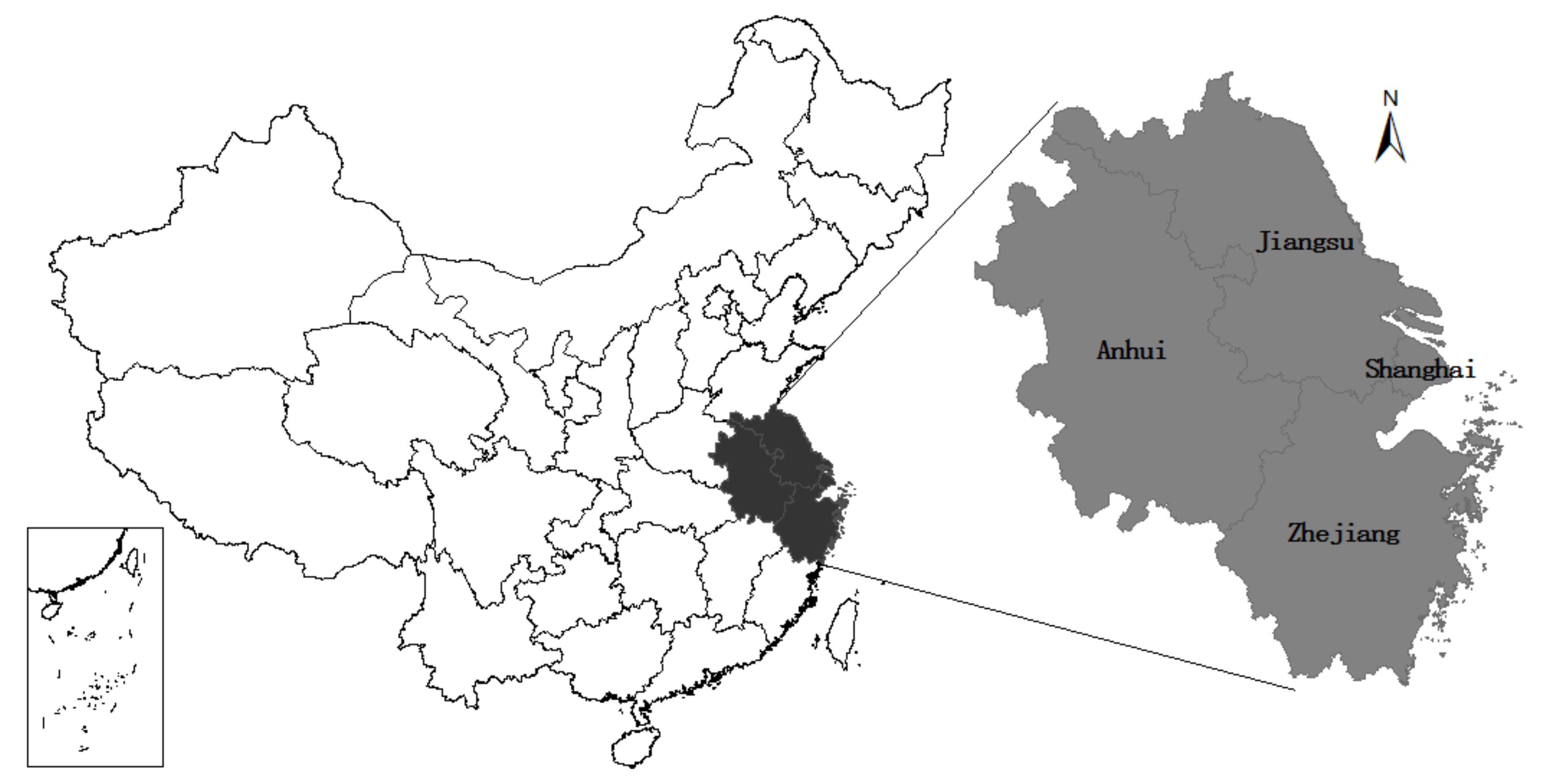
2.1. Research Area

The YRD region is situated on the eastern coast of mainland China, including Shanghai, Zhejiang, Jiangsu, and Anhui provinces, accounting for 3.5% of China’s area, as shown in Figure 1. The YRD region is the economic zone with the fastest economic development, the largest scale, and the greatest development potential in China. In 2012, the YRD region accounted for 16.1% of China’s population, created 24.3% of China’s GDP (Gross Domestic Product), and consumed 17.7% of China’s coal [35]. The rapid development of the economy and urbanization has also brought tremendous environmental pressures to the YRD region, severe haze pollution frequently occurs [36,37]. In December 2013, serious "haze" incidents occurred in central and eastern China. The air quality index of Anhui, Jiangsu, Zhejiang, and Shanghai reached six levels of serious pollution. The YRD has become a region with relatively serious haze after the Beijing–Tianjin–Hebei region, and formed a "continuous haze belt" with the Beijing–Tianjin–Hebei region [38]. To curb the increasingly serious situation of air pollution, the China’s State Council issued the Air Pollution Prevention and Control Action Plan (2013–2017) in September 2013, requiring that by 2017, the PM2.5 concentration in the YRD region should be reduced by about 20% compared with that in 2012. In January 2014, Shanghai, Zhejiang, Jiangsu, and Anhui provinces jointly issued the Rules for the Implementation of the Action Plan for the Prevention and Control of Air Pollution in the YRD Region, which calls for strengthening joint prevention and control of air pollution. Total pollutant discharge control is an important measure for environmental management, so reducing primary PM emissions will be an important means of preventing PM pollution. There is an urgent need to explore the influencing mechanism of socio-economic factors contributing to primary PM emissions for formulating effective policies to achieve the goal of the severely polluted air environment in YRD region.

2.2. Data Sources

The time series data used in this study from 1995 to 2014, namely GDP, total population, coal use, energy use, FDI, fixed assets investment (FAI), and the industrial added value, were all gained from China Statistical Yearbook and China Energy Statistical Yearbook, where GDP data is in 108 yuan by taking in constant prices of 1995 for elimination of inflation and the unit of energy use data is in 104 standard coal (tce) calculated by calorific value. Population is counted by 104 and technology level is measured by tce/104 × yuan. The FDI and FAI is measured by million dollars and billion Yuan, respectively. The unit of industrial structure and energy consumption structure is percent. We downloaded the provincial primary PM (PM2.5, PM10, TSP) emissions data during this period of 1995 to 2014 in the YRD region from the Multi-resolution Emission Inventory for China (MEIC: http://www.meicmodel.org), which was developed by Tsinghua University. MEIC is a bottom-up emissions inventory model that includes emissions estimates for more than 700 emitting source categories [39,40]. The anthropogenic PM emission sources are divided into six categories: fixed combustion sources, process sources, mobile sources, solvent sources, agricultural sources, and waste disposal sources. Each type of emission source is divided into four levels according to sector/industry, fuel/product, combustion/process technology, and terminal control technology, and a complete classification system of emission sources is established step by step from the first level to the fourth level. According to emission factors of different emission sources, taking the multiple sources and control technologies into account, a dynamic methodology, namely MEIC, was built to estimate the primary PM emissions.

3. Methodology

3.1. Time Variation Trend (Slope)

Simple linear regression model is the most commonly used method to detect the time changing trends of observed data. Su et al. analyzed the trend of CO2 emission in China by the method [41], and Lu et al. used it to explore the variation trend of soil water, temperature, and precipitation rate [42]. Its basic form is as follows:
S l o p e = n a = 1 n a P a a = 1 n a a = 1 n P a n a = 1 n a 2 a = 1 n a 2
where, n is equal to 20 and indicates the time interval, and Pa represents primary PM emissions in a year.

3.2. Theil Index

We chose the Theil index to analyze the regional differences of primary PM emissions in the YRD. The Theil index was originally used to calculate the difference and inequality of income [43,44]. In recent years, many scholars have also used the Theil index to study regional differences in carbon dioxide emissions and energy consumption. Su et al. applied the Theil index to analyze regional differences in carbon emissions of Chinese cities from 1992 to 2013 [45]. Liu et al. employed the Theil index to explore regional differences in urban household energy consumption of China from 2001 to 2013 [46]. Referring to the research of Su [45] and Liu [46], we constructed the formula for calculating the Theil index of primary PM emissions as follows:
T = i X i X ln X i X P i P
where, T is the Theil index of primary PM emissions in the YRD; X is the total population of the YRD; Xi is the population in the i province; P is the primary PM emissions in the YRD; Pi is the primary PM emissions in the i province. The smaller the Theil index, the smaller the regional difference of primary PM emissions in the YRD and vice versa.

3.3. STIRPAT Model

Ehrlich and Holden established an IPAT (Impact (I) = Population × (P) × Affluence (A) × Technology (T)) model to evaluate the effects of P, A, and T and their interactions on environmental stress in the 1970s [47,48].
I = P × A × T
However, the IPAT model does not take into account the individual impact of different changes in P, A, and T on environment stress. In 2003, on the basis of considering the individual impact of different changes in P, A, and T on environment stress, York et al. established a stochastic form model, namely STIRPAT model [49,50]. The basic form of the model is as follows:
I = a × Pb × Ac × Td × e
where the total population (P), affluence (A), and technology level (T) are regarded as the driving factors of the primary PM emissions (I); a represents the constant; b, c, and d express the coefficients; e indicates the error term.
Equation (4) is obtained from Equation (1) by taking logarithms:
lnI = lna + b × lnP + c × lnA+d × lnT + lne
As the STIRPAT model can take into account the individual impact of different changes in P, A, and T on environment stress and can be extended by incorporating other factors and appropriately decomposing each factor, this method has been widely used in the analysis of influencing factors of energy use or different pollutant discharge. For instance, Shi used a STIRPAT model for revealing the influence degree of population scale on carbon dioxide emissions in several countries [51]. Liddle applied a STIRPAT method for revealing the internal relationship between climate change and urban density [52]. Zhang et al. revealed the influence degree of ICT industry on carbon dioxide emissions from multiple scales by the STIRPAT model [53]. Abdallh et al. combined the STIRPAT model with semi-parametric regression model for revealing the urbanization and CO2 emissions nexus in the Middle East and North Africa (MENA) region [54]. Liu et al. combined the STIRPAT model with the system dynamics model for revealing the major driving force for China’s carbon emissions [55]. Wang et al. quantified the major driving factors for Xinjiang’s CO2 emissions from different development stages by the STIRPAT model [56]. Shuai et al. utilized data from 125 countries to quantify the factors affecting carbon dioxide emissions from different wage levels by the STIRPAT model [57]. Poumanyvong et al. explored the effect of urbanization on national transport and road energy use of 99 countries over the period 1975 to 2005 with consideration of the different development stages by the STIRPAT model [58]. Zhang and Lin applied the STIRPAT model to analyze the impact of urbanization on energy consumption from national and regional levels [59]. Salim and Shafiei utilized the STIRPAT model for exploring the impact of urbanization on renewable and non-renewable energy consumption in the Organization for Economic Co-operation and Development (OECD) countries from 1980 to 2011 [60]. Wang et al. adopted the STIRPAT model for investigating the impact of urbanization on energy consumption with consideration to provincial differences [61]. Liu et al. adopted an extended STIRPAT model to explore the effects of human activity on energy use, industrial exhaust gases, industrial wastewater, and industrial solid waste at the national and regional levels in China from 1990 to 2012 [62]. Guo et al. used the STIRPAT model to reveal the driving factors of industrial wastewater discharge in Guangdong province from 1990 to 2012 [63].
Therefore, some factors, namely, industrial mix (S), foreign direct investment (FDI), fixed assets investment (FAI) and Energy use mix (E), were incorporated to build the extended STIRPAT model. The final STIRPAT model is as follows.
lnI = lna + β1 × lnP + β2 × lnA + β3 × lnT + β4 × lnS+β5 × lnFDI + β6 × lnFAI + β7 × lnE + lne
where I is represented by primary PM emissions (ton); P indicates the total population (104 people). The per capita GDP (Yuan per capita) is used to explore the influence of affluence (A) on primary PM emissions. Energy use per GDP (tce/104 × yuan) is employed for revealing the impact of the technical level (T) on primary PM emissions. S (industrial mix) is expressed as the proportion of industrial increased value to GDP, which is employed to identify the dynamic effects of the industrial structure change on PM emissions. FDI (foreign direct investment) is measured by million dollars, which is applied to reveal the relationship between trade openness and primary PM emissions; FAI refers to the fixed assets investment that is counted by billion Yuan. E (energy use mix) means the ratio of coal use to total energy use, which was adopted for exploring the influences of the energy consumption structure change on PM emissions; β1, β2, β3, β4, β5, β6, β7 are all elastic coefficients.

3.4. Multicollinearity

Multicollinearity refers to the phenomenon that there is a linear correlation between independent variables. Multicollinearity can be divided into two categories: a set of explanatory variables X1, X2,… Xk, if there are some constants C0, C1,… Ck, resulting in C1 X1 + C2 X2 + … + Ck Xk = 0, this phenomenon is called perfect multicollinearity among independent variables and its correlation coefficient is 1. If there are some constants C0, C1,… Ck, resulting in C1 X1 + C2 X2 + … + Ck Xk + ε = 0, this phenomenon is called approximation multicollinearity. If there exists multicollinearity among explanatory variables in the linear regression model, it will lead to: (1) the variance of ordinary least square (OLS) estimator will increase and the estimation accuracy of parameters will be lower; (2) It is impossible to judge the individual influence of variables; (3) The significance test of variables is meaningless; (4) The regression model is invalid and lacks stability. The variance inflation factor (VIF) calculated based on the OLS regression method is the most commonly used method for diagnosing the existence of multicollinearity. The bigger the VIF, the more serious the multicollinearity. If 0 < VIF < 10, there is no multicollinearity; if 10≤VIF, there is strong multicollinearity.

3.5. Ridge Regression

In 1970, Hoerl and Kennard proposed the ridge regression method systematically [64]. The ridge regression is a biased estimation method based on the OLS regression. Furthermore, it is an improvement of the OLS regression method. The regression method is frequently used in the analysis of collinear data. For instance, Wang et al. applied ridge regression to eliminate multicollinearity for revealing the influence mechanism of socio-economic factors on energy-related carbon dioxide emissions in Guangdong Province, China [65]. Li et al. utilized ridge regression to avoid the multicollinearity of independent variables for understanding the driving factors of the air pollution (SO2, CO2) in Beijing, China [66].
If there is multicollinearity among independent variables, the value of determinant of XTX matrix is approximately 0. If XTX is added to the constant matrix KI (k ≥ 0, the sensitivity of (XTX + KI)−1 will be improved. The estimator of ridge regression is as follows:
β(K) = (XTX + KI)−1 × XTY
If K = 0, the estimator of ridge regression is the result of OLS regression; If K→∞, the estimator of ridge regression is approximate to 0, so K should not be too big.

4. Results

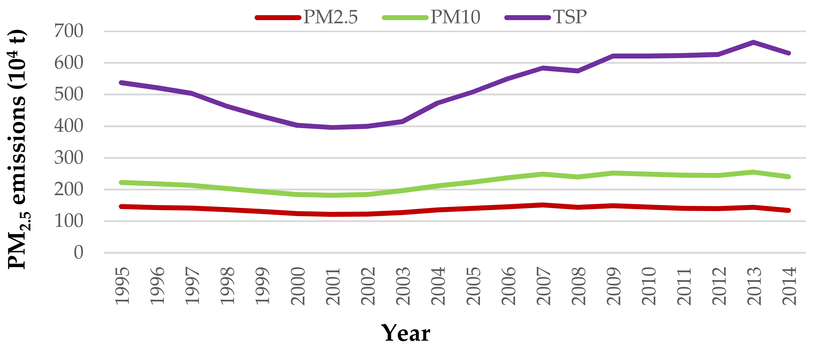
4.1. The Time Variation of Primary PM Emissions

The primary PM2.5, PM10, TSP emissions in the YRD region from 1995 to 2014 are displayed in Figure 2. During this period, the primary PM2.5, PM10, TSP emissions in the YRD region all showed an overall increasing trend, their Slope is 0.40, 3.08, and 11.16, respectively, which indicated that the primary TSP emission had the fastest growth. The growth rate of primary PM10 emission was second. Primary PM2.5 emission grew slowly and remained basically unchanged. However, there all existed large fluctuations during the period (Figure 3). From 1995 to 2001, the primary PM2.5, PM10, TSP emissions in the YRD region all presented a downward trend. However, there are obvious differences on the changes of primary PM2.5, PM10, TSP emissions from 2001 to 2014. Primary PM2.5, PM10, and TSP emissions all featured an uptrend during this period. This may be due to China’s accession to World Trade Organization (WTO) in 2001. After China’s accession to WTO, China’s economy has grown rapidly and energy consumption has increased, which leads to the increase of primary PM emissions.

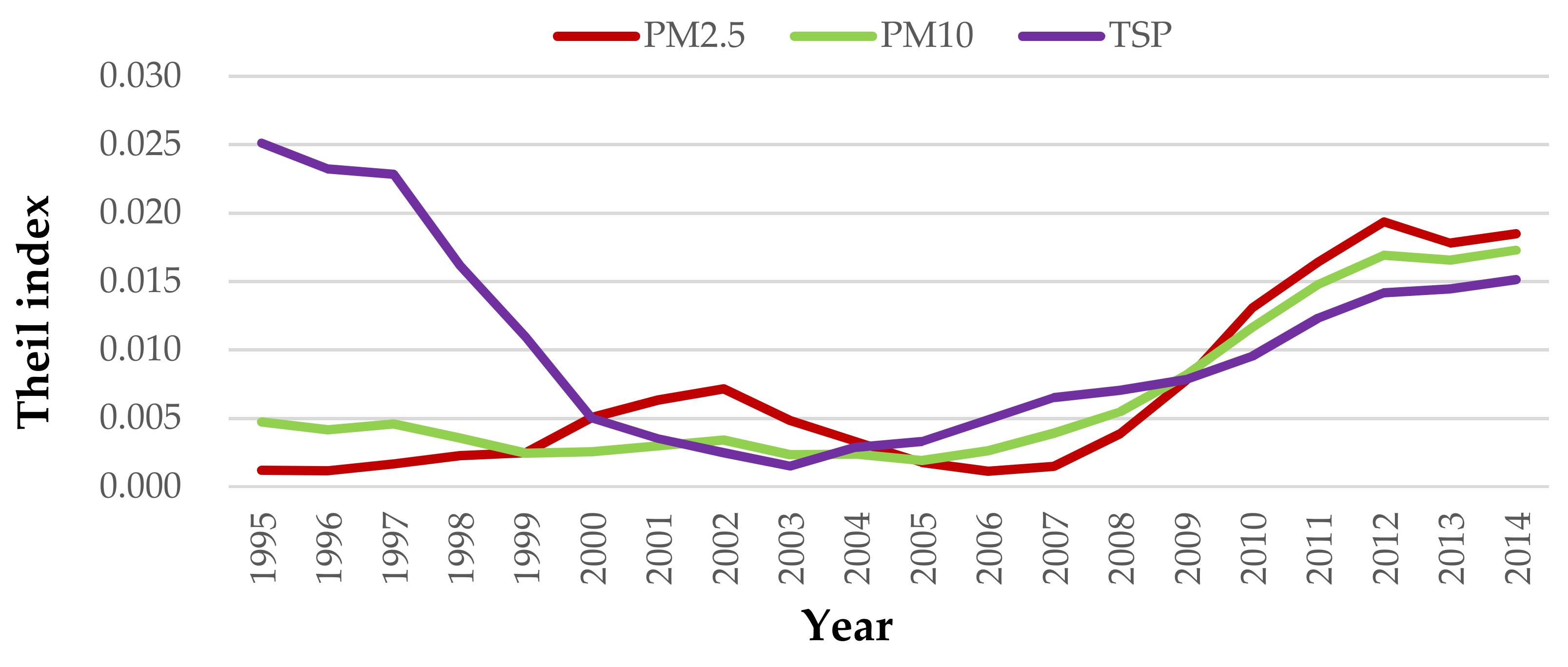
4.2. The Regional Differences in Primary PM Emissions

For the primary PM2.5 emissions, the regional differences in the YRD region increased from 1995 to 2014, and the changing trend of the Theil index was 0.009/10a, but there were large fluctuations during the period (Figure 3). During this period from 1995 to 2002, the regional differences tend showed an upward trend, and the Theil index increased from 0.0012 to 0.0072. The Chinese government was unaware of the harm of PM2.5 pollution during this period primary, and PM2.5 emissions were not restricted. The regional differences reduced from 2002 to 2006, and Theil index decreased from 0.0072 to 0.0011. China entered WTO in 2001, in the early stage of China’s accession to the WTO, the effect of improving emission efficiency was greater than that of economic growth on primary PM2.5 emissions. During this period from 2006 to 2012, the regional differences featured an uptrend, Theil index increased from 0.0011 to 0.0194. As the process of industrialization and urbanization has been expedited, the effect of economic growth was greater than that of improving emission efficiency on primary PM2.5 emissions. Theil index decreased to 0.0185 in 2014, which represents that the regional differences narrowed from 2012 to 2014. Since 2012, the Chinese government has promulgated a series of policies and measures for energy conservation and PM2.5 emission reduction.
For the primary PM10 emissions, the regional differences in the YRD region featured an increasing trend from 1995 to 2014, and the variation trend of Theil index was 0.007/10a, but there was large volatility during the period (Figure 3). From 1995 to 2005, the Theil index decreased by 0.0028, which indicated that the regional differences presented a downward trend. Since 1995, China government has shut down a large number of small enterprises with high energy consumption and pollution, and in the early stage of China’s accession to the WTO, the effect of improving emission efficiency was greater than that of economic growth on primary PM10 emissions. During this period from 2005 to 2014, the regional differences showed an uptrend, and Theil index increased to 0.0173 in 2014. As the process of industrialization and urbanization has been expedited, the effect of economic growth was greater than that of improving emission efficiency on primary PM10 emissions over the period.
For the primary TSP emissions, the regional differences in the YRD region generally showed a downward trend from 1995 to 2014, and the temporal trend of the Theil index was 0.005/10a, but there existed large volatility during the period (Figure 3). During this period from 1995 to 2003, the regional differences presented a decreasing trend, and Theil index decreased from 0.0251 to 0.0015. This may be due to the closure of a large number of energy-intensive and highly polluting small enterprises in China since 1995, and the effect of improving emission efficiency was greater than that of economic growth on primary TSP emissions from 2001 to 2003 because of China’s accession to the WTO. From 2003 to 2014, the Theil index increased from 0.0015 to 0.0151, which indicated that the regional differences featured an upward trend. With the acceleration of industrialization and urbanization after China’s accession to the WTO, the impact of economic growth on TSP emissions was greater than that of improving emission efficiency from 2003 to 2014.

4.3. Multicollinearity Test Results

The OLS results of primary PM2.5, PM10, TSP emissions in the YRD region from 1995 to 2014 are displayed in Table 1. From Table 1, we found that some VIFs are greater than 10, which indicated that the OLS results of primary PM2.5, PM10, TSP emissions are not reliable. Obviously, we must eliminate multicollinearity between independent variables for getting reliable regression results.

4.4. Empirical Analysis

The ridge regression method was adopted for reducing the impact of multicollinearity between independent variables, the simulation results are shown in Table 2. The coefficients of the ridge regression are selected according to the ridge trace. When K = 0.08 (PM2.5), K = 0.12 (PM10), K = 0.15 (TSP), the ridge trace is almost stable. The specific coefficients are shown in Table 2.
This paper examined the effects of different socio-economic factors on PM (PM2.5, PM10, TSP) emissions from energy consumption. Table 2 shows that population size had a significant positive effect on primary PM emission, similar to the viewpoints of Guan et al. [31] and Lyu et al. [34]. Generally speaking, the increase of population size can affect PM emission in the following two ways: one is the agglomeration effect, the other is the scale effect. Increasing population size often produces an agglomeration effect, which will improve technological level, public transport sharing efficiency, and energy efficiency to reduce PM emissions. On the other hand, the increase in population size will directly or indirectly lead to an increase in energy consumption, thus, increasing PM emissions. Estimated results showed that the scale effect of population size is significantly higher than that of the agglomeration effect. Therefore, the government should pay more attention to the effect of population agglomeration on primary PM emissions in the future. For example, advocating low-energy transportation will be a good measure to reduce primary PM emissions. That is, primary PM emissions in transportation can be effectively controlled by speeding up the transformation of transportation development mode and promoting the construction of energy-saving comprehensive transportation system. Furthermore, residents’ awareness of energy conservation and environmental protection should be improved by publicizing a low-energy life concept. The government should also guide residents to change their high-energy consumption habits by some economic incentives.
The negative effect of economic growth on energy PM emissions was significant, contrary to the viewpoints of Guan et al. [31] and Lyu et al. [34]. Generally speaking, economic growth can affect PM emissions through the following three aspects. (1) Scale effect. Economic growth needs to increase input, thereby, increasing energy use, and more output will inevitably lead to an increase in pollution emissions. (2) Technical effect. High-income level is closely related to better environmental protection technology and high -efficiency technology. In the course of economic growth, the increase of research and development (R&D) expenditure and the promotion of technological progress have two effects: One is that technological progress improves productivity, the efficiency of resource utilization, and reduces the input of elements per unit output; the other is that clean technology is continuously developed. It reduces the pollution emission per unit output. (3) Structural effects. In the early stage, the economic structure changed from agriculture to energy-intensive heavy industry, increasing pollution emissions. Subsequently, the economic structure shifted to low-polluting services and knowledge-intensive industries, with pollution emission per unit output declining and environmental quality improving. The simulation coefficients showed that the technological and scale effects of the economic growth in the YRD region won during the research period. Therefore, the government should adhere to green, sustainable development and achieve a win–win situation of stable economic growth and continuous decline in PM emissions.
The increase in the proportion of secondary industry had a significant positive effect on PM emission. This is consistent with the viewpoint of Lyu et al. [34] that economic activities from the secondary sector resulted in the growth of air pollutant emissions. With the high advancement of industrialization, secondary industry becomes the main driving force of economic development. The industrial structure dominated by secondary industry was also the main factor leading to primary PM emissions. The result of upgrading of industrial structure is that under the influence of technological progress, the industry continuously eliminates outdated capacity, and develops a technology-intensive industry with high technology content. Therefore, promoting the optimization, transformation, and upgrading of industrial structure and developing green industry will be effective measures to reduce PM emissions.
The increase of FDI had different effects on primary PM2.5, PM10, and TSP emissions. On the one hand, some scholars believe that FDI can improve energy efficiency by introducing more environmentally technologies, thereby, reducing pollution emissions from energy use; on the other hand, some scholars believe that the introduction of FDI will transfer pollution emissions to the host country through high energy consumption and high emission industries, thereby, increasing pollution emissions from energy use. The estimated coefficient of FDI is significantly positive for primary PM2.5 emissions under the level α = 0.1, whereas the impact of FDI on primary PM10 and TSP emissions were all statistically not significant even under the level α = 0.1. Therefore, when introducing FDI, the Chinese government needs to screen it, raises its environmental access threshold, and give full play to the role of FDI in improving environmental quality.
The estimated coefficient of FAI was significantly positive at the level of 1%, which indicated that the increase of FAI increased primary PM emissions. This is consistent with the viewpoint of Xu et al. [33] that investments featured a positive effect on primary air pollutant emissions. The swift growth of China’s economy is investment-driven. The investments in fixed assets in China are mainly concentrated in the secondary industry, resulting in the largest primary PM emissions compared with the first and third industries. The extensive investments in the secondary industry are not conducive to industrial restructuring and upgrading. These investments are mainly used to promote production technology progress rather than green technology progress, which leads to the expansion of production scale and has a positive effect on primary PM emissions. Therefore, the Chinese government needs to make low-energy screening for FAI, improve the environmental access threshold of investment, and use more investments to promote green technology progress for reducing primary PM emissions.
The estimated coefficient of energy structure was significantly positive at the level of 1%, which indicated that the increase in coal proportion increases primary PM emissions. Therefore, in the future, it is urgent to optimize the energy consumption structure, improve the utilization rate of clean energy, reduce the proportion of coal use, so as to reduce primary PM emissions from energy consumption. In addition, the influence of energy intensity on PM emission from energy consumption is mainly negative but not significant even under the level of 10%. Therefore, the government needs to increase investment in scientific research and develop PM emission reduction technologies.

5. Conclusions

Haze pollution in the YRD region is getting worse with the rapid development of the economy, which is harmful to human health. To understand and control haze pollution in the YRD region, the temporal trend of primary PM emission in the YRD from 1995 to 2014 was explored by the Slope method. Then, the regional differences of primary PM emissions in the YRD were analyzed by the Theil index from 1995 to 2014. Finally, an extended STIRPAT model was adopted for quantitatively revealing the effect of various socio-economic factors contributing to primary PM emissions in the YRD region during 1995–2014 and some conclusions have been drawn. Primary PM2.5, PM10, TSP emissions all featured an uptrend, which showed that haze pollution in the YRD region showed a deteriorating trend over the study period. The regional differences of primary TSP emissions in the YRD region were gradually shrinking, and the regional differences of primary PM2.5 and PM10 emissions in the YRD region presented a rising trend of fluctuation. The estimated coefficient of population size, energy structure, and FAI were all significantly positive at the level of 1%, which indicated that the increase of population, coal proportion, the proportion of secondary industry, and FAI increased primary PM emissions. The negative effect of economic growth on energy PM emissions was significant under the level of 1%. The increase of FDI had different effects on primary PM2.5, PM10 and TSP emissions. The estimated coefficient of FDI is significantly positive for primary PM2.5 emissions under the level α = 0.1, whereas the impact of FDI on primary PM10 and TSP emissions were all statistically not significant even under the level α = 0.1. Moreover, the influence of energy intensity on primary PM emission from energy consumption is mainly negative but not significant even under the level of 0.1. The above conclusions are of great policy significance for the realization of primary PM emissions reduction in the YRD region through socio-economic means. Therefore, to achieve the goal of primary PM emissions reduction, YRD region should continue to optimize its industrial structure, streamline extensive investment, rationally adjust its energy consumption structure, and increase its R&D intensity.

Author Contributions

H.X. and G.J. designed this study. H.W. contributed the data used in this study and analyzed the data. G.J. and H.X. participated in the analysis and presentation of results. H.X. contributed an original draft of the paper. G.J. and H.X. contributed writing—review & editing.

Funding

This work was supported by the project of the National Natural Science Foundation of China (grant number 41401657) and the National Key Research and Development Program of China (grant number 2017YFE0100700).

Conflicts of Interest

The authors declare no conflict of interest.

References

  1. Li, L.; Chen, C.; Huang, C.; Huang, H.; Li, Z.; Fu, J.S.; Jang, C.J.; Streets, D.G. Regional air pollution characteristics simulation of O3 and PM10 over Yangtze River Delta Region. Environ. Sci. 2008, 29, 237–245. (In Chinese) [Google Scholar]
  2. Geng, G.; Zhang, Q.; Martin, R.V.; Donkelaar, A.V.; Huo, H.; Che, H.; Lin, J.; He, K. Estimating long-term PM2.5 concentrations in China using satellite-based aerosol optical depth and a chemical transport model. Remote Sens. Environ. 2015, 166, 262–270. [Google Scholar] [CrossRef]
  3. Tian, S.; Pan, Y.; Liu, Z.; Wen, T.; Wang, Y. Size-resolved aerosol chemical analysis of extreme haze pollution events during early 2013 in urban Beijing, China. J. Hazard. Mater. 2014, 279, 452–460. [Google Scholar] [CrossRef] [PubMed]
  4. Feng, Y.; Chen, Y.; Guo, H.; Zhi, G.; Xiong, S.; Sheng, G.; Fu, J. Characteristics of organic and elemental carbon in PM2.5 samples in Shanghai, China. Atmos. Res. 2009, 92, 434–442. [Google Scholar] [CrossRef]
  5. Shen, G.F.; Yuan, S.Y.; Xie, Y.N.; Xia, S.J.; Li, L.; Yao, Y.K.; Qiao, Y.Z.; Zhang, J.; Zhao, Q.Y.; Ding, A.J.; et al. Ambient levels and temporal variations of PM2.5 and PM10 at a residential site in the mega-city, Nanjing, in the western Yangtze River Delta, China. J. Environ. Sci. Health A Toxic Hazard. Substain. Environ. Eng. 2014, 49, 171–178. [Google Scholar] [CrossRef]
  6. Wang, M.; Cao, C.; Li, G.; Singh, R.P. Analysis of a severe prolonged regional haze episode in the Yangtze River Delta, China. Atmos. Environ. 2015, 102, 112–121. [Google Scholar] [CrossRef]
  7. Xu, J.; Yan, F.; Xie, Y.; Wang, F.; Wu, J.; Fu, Q. Impact of meteorological conditions on a nine-day particulate matter pollution event observed in December 2013, Shanghai, China. Particuology 2015, 20, 69–79. [Google Scholar] [CrossRef]
  8. Lou, C.R.; Liu, H.Y.; Li, Y.F.; Li, Y.L. Socioeconomic Drivers of PM2.5 in the Accumulation Phase of Air Pollution Episodes in the Yangtze River Delta of China. Int. J. Environ. Res. Public Health 2016, 13, 928. [Google Scholar] [CrossRef]
  9. Dockery, D.W.; Pope, C.A.; Xu, X.; Spengler, J.D.; Ware, J.H.; Fay, M.E.; Ferris, B.G.; Speizer, F.E. An association between air pollution and mortality in six US cities. N. Engl. J. Med. 1993, 329, 1753–1759. [Google Scholar] [CrossRef]
  10. Pope, C.A., III. Review: Epidemiological basis for particulate air pollution health standards. Aerosol. Sci. Technol. 2000, 32, 4–14. [Google Scholar] [CrossRef]
  11. Pope, C.A., III; Burnett, R.T.; Thun, M.J.; Calle, E.E.; Krewski, D.; Ito, K.; Thurston, G.D. Lung cancer, cardiopulmonary mortality, and long-term exposure to fine particulate air pollution. JAMA 2002, 287, 1132–1141. [Google Scholar] [CrossRef]
  12. Franklin, M.; Koutrakis, P.; Schwartz, P. The role of particle composition on the association between PM 2.5 and mortality. Epidemiology 2008, 19, 680–689. [Google Scholar] [CrossRef]
  13. Delfino, R.J.; Sioutas, C.; Malik, S. Potential role of ultrafine particles in associations between airborne particle mass and cardiovascular health. Environ. Health Perspect. 2005, 113, 934–946. [Google Scholar] [CrossRef]
  14. Laden, F.; Neas, L.M.; Dockery, D.W.; Schwartz, J. Association of fine particulate matter from different sources with daily mortality in six US cities. Environ. Health Perspect. 2000, 108, 941–947. [Google Scholar] [CrossRef]
  15. Laden, F.; Schwartz, J.; Speizer, F.E.; Dockery, D.W. Reduction in fine particulate air pollution and mortality: Extended follow-up of the Harvard six cities study. Am. J. Respir. Crit. Care Med. 2006, 173, 667–672. [Google Scholar] [CrossRef]
  16. Samet, J.M.; Dominici, F.; Curriero, F.C.; Coursac, I.; Zeger, S.L. Fine particulate air pollution and mortality in 20 U.S. cities, 1987–1994. N. Engl. J. Med. 2000, 343, 1742–1749. [Google Scholar] [CrossRef]
  17. Wang, H.; Dwyer-Lindgren, L.; Lofgren, K.T.; Rajaratnam, J.K.; Marcus, J.R.; Levin-Rector, A.; Levitz, C.E.; Lopez, A.D.; Murray, C.J.L. Age specific and sex-specific mortality in 187 countries, 1970–2010: A systematic analysis for the global burden of disease study 2010. Lancet 2012, 380, 2071–2094. [Google Scholar] [CrossRef]
  18. Pope, C.A., 3rd; Thun, M.J.; Namboodiri, M.M.; Dockery, D.W.; Evans, J.S.; Speizer, F.E.; Heath, C.W. Particulate air pollution as a predictor of mortality in a prospective study of U.S. adults. Am. J. Respir. Crit. Care Med. 1995, 151, 669–674. [Google Scholar] [CrossRef]
  19. Du, X.; Kong, Q.; Ge, W.; Zhang, S.; Fu, L. Characterization of personal exposure concentration of fine particles for adults and children exposed to high ambient concentrations in Beijing, China. J. Environ. Sci. 2010, 22, 1757–1764. [Google Scholar] [CrossRef]
  20. Zhang, H.; Tripathi, N.K. Geospatial hot spot analysis of lung cancer patients correlated to fine particulate matter (PM2.5) and industrial wind in eastern Thailand. J. Clean. Prod. 2018, 170, 407–424. [Google Scholar] [CrossRef]
  21. Han, L.; Zhou, W.; Li, W. City as a major source area of fine particulate (PM2.5) in China. Environ. Pollut. 2015, 206, 183–187. [Google Scholar] [CrossRef]
  22. Tan, J.; Zhang, L.; Zhou, X.; Duan, J.; Li, Y.; Hu, J.; He, K. Chemical characteristics and source apportionment of PM2.5 in Lanzhou, China. Sci. Total Environ. 2017, 601–602, 1743–1752. [Google Scholar] [CrossRef]
  23. Qiao, X.; Ying, Q.; Li, X.; Zhang, H.; Hu, J.; Tang, Y.; Chen, X. Source apportionment of PM2.5 for 25 Chinese provincial capitals and municipalities using a source-oriented community multiscale air quality model. Sci. Total Environ. 2018, 612, 462–471. [Google Scholar] [CrossRef]
  24. Olvera, H.A.; Garcia, M.; Li, W.; Yang, H.; Amaya, M.A.; Myers, O.; Burrchiel, S.W.; Berwick, M.; Pingtore, N.E. Principal Component Analysis Optimization of a PM2.5 Land Use Regression Model with Small Monitoring Network. Sci. Total Environ. 2012, 425, 27–34. [Google Scholar] [CrossRef]
  25. Zou, B.; Luo, Y.; Wan, N.; Zheng, Z.; Sternberg, T.; Liao, Y. Performance comparison of LUR and OK in PM2.5 concentration mapping: A multidimensional perspective. Sci. Rep. 2015, 5, 8698. [Google Scholar] [CrossRef] [PubMed]
  26. Wang, S.; Zhou, C.; Wang, Z.; Feng, K.; Hubacek, K. Characteristics and drivers of fine particulate matter (PM2.5) distribution in China. J. Clean. Prod. 2017, 142, 1800–1809. [Google Scholar] [CrossRef]
  27. Yang, G.; Huang, J.; Li, X. Mining sequential patterns of PM2.5 pollution in three zones in China. J. Clean. Prod. 2018, 170, 388–398. [Google Scholar] [CrossRef]
  28. Li, G.; Fang, C.; Wang, S.; Sun, S. The effect of economic growth, urbanization, and industrialization on fine particulate matter (PM2.5) concentrations in China. Environ. Sci. Technol. 2016, 50, 11452–11459. [Google Scholar] [CrossRef] [PubMed]
  29. Hao, Y.; Liu, Y.M. The influential factors of urban PM2.5, concentrations in China: A spatial econometric analysis. J. Clean. Prod. 2016, 112, 1443–1453. [Google Scholar] [CrossRef]
  30. Jiang, P.; Yang, J.; Huang, C.; Liu, H. The contribution of socioeconomic factors to PM2.5 pollution in urban China. Environ. Pollut. 2018, 233, 977–985. [Google Scholar] [CrossRef]
  31. Guan, D.B.; Su, X.; Zhang, Q.; Peters, G.P.; Liu, Z.; Lei, Y.; He, K. The socioeconomic drivers of China’s primary PM2.5 emissions. Environ. Res. Lett. 2014, 9, 024010. [Google Scholar] [CrossRef]
  32. Meng, J.; Liu, J.; Guo, S.; Huang, Y.; Tao, S. The impact of domestic and foreign trade on energy-related pm emissions in Beijing. Appl. Energy 2016, 184, 853–862. [Google Scholar] [CrossRef]
  33. Lyu, W.; Li, Y.; Guan, D.; Zhao, H.; Zhang, Q.; Liu, Z. Driving forces of chinese primary air pollution emissions: An index decomposition analysis. J. Clean. Prod. 2016, 133, 136–144. [Google Scholar] [CrossRef]
  34. Xu, S.; Zhang, W.; Li, Q.; Zhao, B.; Wang, S.; Long, R. Decomposition analysis of the factors that influence energy-related air pollutant emission changes in China using the SDA method. Sustainability 2017, 9, 1742. [Google Scholar] [CrossRef]
  35. Li, L.; An, J.Y.; Lu, Q. Modeling Assessment of PM2.5 Concentrations Under Implementation of Clean Air Action Plan in the Yangtze River Delta Region. Res. Environ. Sci. 2015, 28, 1653–1661. [Google Scholar]
  36. Fu, Q.; Zhuang, G.; Wang, J.; Xu, C.; Huang, K.; Li, J.; Hou, B.; Lu, T.; Streets, D.G. Mechanism of formation of the heaviest pollution episode ever recorded in the Yangtze River Delta, China. Atmos. Environ. 2008, 42, 2023–2036. [Google Scholar] [CrossRef]
  37. Ming, L.; Jin, L.; Li, J.; Fu, P.; Yang, W.; Liu, D.; Zhang, G.; Wang, Z.; Li, X. PM2.5 in the Yangtze River Delta, China: Chemical compositions, seasonal variations, and regional pollution events. Environ. Pollut. 2017, 223, 200–212. [Google Scholar] [CrossRef]
  38. Mi, K.; Zhuang, R.; Liang, L.; Duan, Y.; Gao, J. Spatio-temporal evolution and characteristics of PM2.5 in the Yangtze River Delta based on real-time monitoring data during 2013–2016. Geogr. Res. 2018, 37, 1641–1654. (In Chinese) [Google Scholar]
  39. Zhang, Q.; Streets, D.G.; He, K.; Wang, Y.; Richter, A.; Burrows, J.P.; Uno, I.; Jang, C.J.; Chen, D.; Yao, Z.; et al. NOx emission trends for China, 1995–2004: The view from the ground and the view from space. J. Geophys. Res. 2007, 112. [Google Scholar] [CrossRef]
  40. Lei, Y.; Zhang, Q.; He, K.B.; Streets, D.G. Primary anthropogenic aerosol emission trends for China, 1990–2005. Atmos. Chem. Phys. 2011, 11, 931–954. [Google Scholar] [CrossRef] [Green Version]
  41. Su, Y.; Chen, X.; Li, Y.; Liao, J.; Ye, Y.; Zhang, H.; Huang, N.; Kuang, Y. China’s 19-year city-level carbon emissions of energy consumptions, driving forces and regionalized mitigation guidelines. Renew. Sustain. Energy Rev. 2014, 35, 231–243. [Google Scholar] [CrossRef]
  42. Lu, H.; Shi, J. Reconstruction and analysis of temporal and spatial variations in surface soil moisture in China using remote sensing. Chin. Sci. Bull. 2012, 57, 1412–1422. (In Chinese) [Google Scholar] [CrossRef]
  43. Theil, H. Economics and Information Theory; North Holland Publishing Company: Amsterdam, The Netherlands, 1967. [Google Scholar]
  44. Akita, T. Decomposing regional income inequality in China and Indonesia using two-stage nested Theil decomposition method. Ann. Reg. Sci. 2003, 33, 55–77. [Google Scholar] [CrossRef]
  45. Su, W.; Liu, Y.; Wand, S.; Zhao, Y.; Su, Y.; Li, S. Regional inequality, spatial spillover effects, and the factors influencing city-level energy-related carbon emissions in China. J. Geogr. Sci. 2018, 28, 495–513. [Google Scholar] [CrossRef]
  46. Liu, M.; Liu, X. Regional Difference of Urban Household Energy Consumption and Contribution Degree in China: A study based on the Theil Index method. J. Guizhou Univ. Financ. Econ. 2017, 2, 1–9. (In Chinese) [Google Scholar]
  47. Ehrlich, P.R.; Holdren, J.P. Impact of population growth. Science 1971, 171, 1212–1217. [Google Scholar] [CrossRef]
  48. Holdren, J.P.; Ehrlich, P.R. Human population and the global environment. Am. Sci. 1974, 62, 282. [Google Scholar]
  49. York, R.; Rosa, E.A.; Dietz, T. Footprints on the Earth: The environmental consequences of modernity. Am. Sociol. Rev 2003, 68, 279–300. [Google Scholar] [CrossRef]
  50. York, R.; Rosa, E.A.; Dietz, T. STIRPAT, IPAT and ImPACT: Analytic tools for unpacking the driving forces of environmental impacts. Ecol. Econ. 2003, 46, 351–365. [Google Scholar] [CrossRef]
  51. Shi, A. The impact of population pressure on global carbon dioxide emissions, 1975–1996: Evidence from pooled cross-country data. Ecol. Econ. 2003, 44, 24–42. [Google Scholar] [CrossRef]
  52. Liddle, B. Urban density and climate change: A STIRPAT analysis using city-level data. J. Transp. Geogr. 2013, 28, 22–29. [Google Scholar] [CrossRef]
  53. Zhang, C.; Liu, C. The impact of ICT industry on CO2 emissions: A regional analysis in China. Renew. Sustain. Energy Rev. 2015, 44, 12–19. [Google Scholar] [CrossRef]
  54. Abdallh, A.A.; Abugamos, H. A semi-parametric panel data analysis on the urbanisation-carbon emissions nexus for the MENA countries. Renew. Sustain. Energy Rev. 2017, 78, 1350–1356. [Google Scholar] [CrossRef]
  55. Liu, D.; Xiao, B. Can China achieve its carbon emission peaking? A scenario analysis based on stirpat and system dynamics model. Ecol. Indic. 2018, 93, 647–657. [Google Scholar] [CrossRef]
  56. Wang, C.; Wang, F.; Zhang, X.; Yang, Y.; Su, Y.; Ye, Y.; Zhang, H. Examining the driving factors of energy related carbon emissions using the extended STIRPAT model based on IPAT identity in Xinjiang. Renew. Sustain. Energy Rev. 2017, 67, 51–61. [Google Scholar] [CrossRef]
  57. Shuai, C.; Shen, L.; Jiao, L.; Wu, Y.; Tan, Y. Identifying key impact factors on carbon emission: Evidences from panel and time-series data of 125 countries from 1990 to 2011. Appl. Energy 2017, 187, 310–325. [Google Scholar] [CrossRef]
  58. Poumanyvong, P.; Kaneko, S.; Dhakal, S. Impacts of urbanization on national transport and road energy use: Evidence from low, middle and high income countries. Energy Policy 2012, 46, 268–277. [Google Scholar] [CrossRef]
  59. Zhang, C.; Lin, Y. Panel estimation for urbanization, energy consumption and CO2; emissions: A regional analysis in China. Energy Policy 2012, 49, 488–498. [Google Scholar] [CrossRef]
  60. Salim, R.A.; Shafiei, S. Urbanization and renewable and non-renewable energy consumption in OECD countries: An empirical analysis. Econ. Model. 2014, 38, 581–591. [Google Scholar] [CrossRef]
  61. Wang, Q.; Wu, S.; Zeng, Y.; Wu, B. Exploring the relationship between urbanization, energy consumption, and CO2 emissions in different provinces of China. Renew. Sustain. Energy Rev. 2016, 54, 1563–1579. [Google Scholar] [CrossRef]
  62. Liu, Y.; Zhou, Y.; Wu, W. Assessing the impact of population, income and technology on energy consumption and industrial pollutant emissions in China. Appl. Energy 2015, 155, 904–917. [Google Scholar] [CrossRef] [Green Version]
  63. Guo, W.; Zhou, Y.; Kan, X. Characteristics and Driving Factors of Wastewater Emissions in Guangdong Province from 1990 to 2012: A Study based on STIRPAT Model and Decoupling Index. J. Irrig. Drain. 2015, 34, 7–10. (In Chinese) [Google Scholar]
  64. Hoerl, A.; Kennard, R. Ridge regression: Biased estimation for nonorthogonal problems. Technometrics 1970, 12, 55–67. [Google Scholar] [CrossRef]
  65. Wang, P.; Wu, W.; Zhu, B.; Wei, Y. Examining the impact factors of energy-related CO2 emissions using the STIRPAT model in Guangdong Province, China. Appl. Energy 2013, 106, 65–71. [Google Scholar] [CrossRef]
  66. Li, W.; Sun, S. Air pollution driving factors analysis: Evidence from economically developed area in China. Environ. Prog. Sustain. Energy 2016, 35, 1231–1239. [Google Scholar] [CrossRef]
Figure 1. The spatial distribution of research area.
Sustainability 11 02269 g001
Figure 2. Time variations of primary particulate matter (PM) emissions in Yangtze River Delta (YRD) region.
Sustainability 11 02269 g002
Figure 3. Theil index of primary PM emissions in the YRD region.
Sustainability 11 02269 g003
Table 1. Ordinary least square (OLS) results.
PM2.5PM10TSP
Unstandardized CoefficientsVIFUnstandardized CoefficientsVIFUnstandardized CoefficientsVIF
lnP1.880121.1032.107121.1032.058121.103
lnA1.325658.8561.778658.8561.927658.856
lnT0.6829.6900.7759.6900.8049.690
lnS0.8141.9560.9071.9561.1071.956
lnFDI−0.09214.313−0.09114.313−0.09414.313
lnFAI–1.049683.597−1.372683.597−1.430683.597
lnE−0.22117.816−0.30117.816−0.23217.816
C−11.723 −15.789 −16.658
R20.988 0.983 0.947
F test853.465 590.062 183.261
Sig.0.000 0.000 0.000
Note: Sig. represents the statistical significance of the simulation formulas.
Table 2. Ridge regression results.
CoefficientPM2.5PM10TSP
lnP0.843 *** (33.469)0.779 *** (28.414)0.672 *** (19.719)
lnA−0.101 *** (−6.416)−0.075 *** (−4.762)−0.045 *** (−2.408)
lnT0.011 (0.156)−0.064 (−0.910)−0.085 (−1.000)
lnS0.620 *** (6.569)0.664 *** (6.061)0.807 *** (5.733)
lnFDI−0.027 * (−1.813)−0.006 (−0.433)0.007 (0.405)
lnFAI0.087 *** (5.887)0.095 *** (6.627)0.097 *** (5.798)
lnE0.608 *** (8.195)0.689 *** (8.752)0.713 * (7.456)
C4.348 *** (2.801)1.396 *** (2.606)2.095 ***(3.098)
R20.9730.9560.913
F test369.547227.404107.583
Sig.0.0000.0000.000
K0.080.120.15
Notes: *, ** and *** indicate statistical significance at the 1%, 5%, and 10% level. t-Statistics are in parentheses.

