Estimation of Gridded Population and GDP Scenarios with Spatially Explicit Statistical Downscaling


Abstract
:1. Introduction
2. Downscale Approach
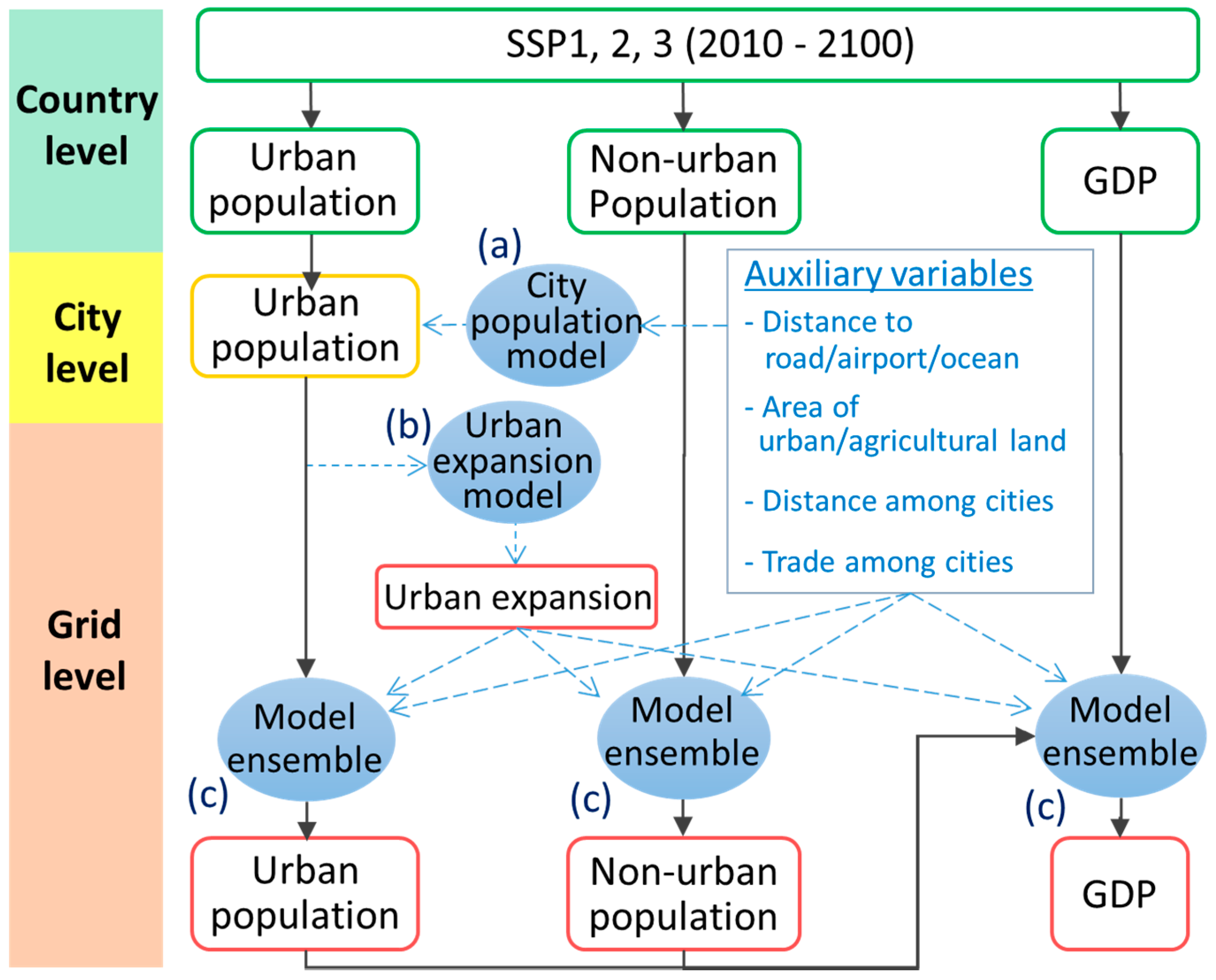
2.1. Overview
2.2. City Growth Model: Estimation with Current Data
2.3. Overview
2.4. Projection of Urban Area
2.5. Downscale Approach
3. Result
3.1. Parameter Estimation Result
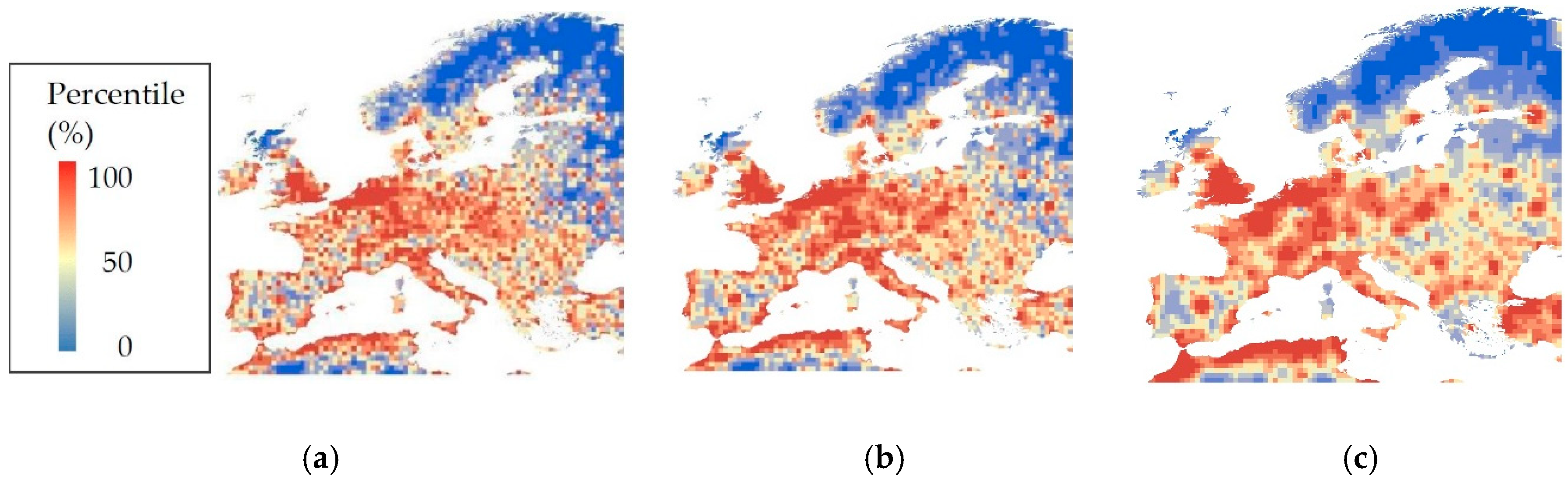
3.2. Downscaling Result
4. Concluding Remarks
Author Contributions
Funding
Conflicts of Interest
Appendix A. Details of the Downscaling Approach
A.1. Projection of Urban Population and Urban Expansion
City Growth Model: Model
City Growth Model: Estimation

| Estimate | t-value | |||
|---|---|---|---|---|
| Intercept | −6.19×10⁻⁴ | −8.12 | *** | |
| α | 1.87×10⁻³ | 8.98 | *** | |
| ρgeo | 9.56×10⁻¹ | 188.57 | *** | |
| ρe1 | 1.83×10⁻³ | 24.95 | *** | |
| ρe2 | 4.10×10⁻⁴ | 0.84 | ||
| βroad | 1.21×10⁻³ | 3.46 | *** | |
| βocean | 2.10×10⁻⁴ | 2.19 | *** | |
| βairport | −1.66×10⁻⁴ | −0.47 | ||
| r | 209 | |||
| Quasi-adjusted R2 | for Δpt+5 | 0.405 | ||
| for pt+5 | 0.998 | |||
City Growth Model: Application for City Population Projections
Projection of Urban Potentials
Projection of Urban Area
A.2. Downscale Approach
| Baseline Variables | Urban Area | Urban Pop | Urban Potential | ||||||||||||||
| Control Variables | 1 | Road | Air | Ocean | 1 | Road | Air | Ocean | 1 | Road | Air | Ocean | |||||
| Urban Population | SSP1 | 0.02 | 0.10 | 0.07 | 0.11 | 0.02 | 0.01 | 0.03 | 0.11 | 0.05 | 0.19 | 0.15 | 0.16 | ||||
| SSP2 | 0.09 | 0.05 | 0.05 | 0.10 | 0.02 | 0.02 | 0.03 | 0.11 | 0.03 | 0.13 | 0.12 | 0.26 | |||||
| SSP3 | 0.07 | 0.03 | 0.05 | 0.10 | 0.08 | 0.07 | 0.06 | 0.08 | 0.03 | 0.04 | 0.13 | 0.28 | |||||
| Baseline Variables | Agri Area | Urban Pop | Urban Potential | ||||||||||||||
| Control Variables | 1 | Road | Air | Ocean | 1 | Road | Air | Ocean | 1 | Road | Air | Ocean | |||||
| Nonurban Population | SSP1 | 0.03 | 0.04 | 0.07 | 0.03 | 0.02 | 0.03 | 0.03 | 0.06 | 0.08 | 0.41 | 0.13 | 0.07 | ||||
| SSP2 | 0.04 | 0.03 | 0.09 | 0.03 | 0.02 | 0.01 | 0.03 | 0.07 | 0.08 | 0.37 | 0.12 | 0.11 | |||||
| SSP3 | 0.07 | 0.02 | 0.10 | 0.04 | 0.01 | 0.01 | 0.03 | 0.09 | 0.05 | 0.17 | 0.19 | 0.23 | |||||
| Baseline Variables | Urban + Agri Area | Urban Pop | Urban Potential | SSP Pop | |||||||||||||
| Control Variables | 1 | Road | Air | Ocean | 1 | Road | Air | Ocean | 1 | Road | Air | Ocean | 1 | Road | Air | Ocean | |
| GDP | SSP1 | 0.07 | 0.01 | 0.04 | 0.05 | 0.18 | 0.10 | 0.14 | 0.04 | 0.06 | 0.03 | 0.03 | 0.04 | 0.02 | 0.06 | 0.09 | 0.04 |
| SSP2 | 0.10 | 0.02 | 0.03 | 0.05 | 0.14 | 0.09 | 0.08 | 0.03 | 0.08 | 0.08 | 0.05 | 0.06 | 0.08 | 0.03 | 0.07 | 0.03 | |
| SSP3 | 0.01 | 0.05 | 0.01 | 0.05 | 0.10 | 0.09 | 0.01 | 0.05 | 0.09 | 0.17 | 0.17 | 0.01 | 0.09 | 0.02 | 0.07 | 0.01 | |
References
- O’Neill, B.C.; Kriegler, E.; Riahi, K.; Ebi, K.L.; Hallegatte, S.; Carter, T.R.; Mathur, R.; van Vuuren, D.P. A new scenario framework for climate change research: The concept of shared socioeconomic pathways. Clim. Chang. 2014, 122, 387–400. [Google Scholar] [CrossRef]
- O’Neill, B.C.; Kriegler, E.; Ebi, K.L.; Kemp-Benedict, E.; Riahi, K.; Rothman, D.S.; van Ruijven, B.J.; van Vuuren, D.P.; Birkmann, J.; Kok, K.; et al. The roads ahead: Narratives for shared socioeconomic pathways describing world futures in the 21st century. Glob. Environ. Chang. 2015, 42, 169–180. [Google Scholar] [CrossRef]
- Gaffin, S.R.; Rosenzweig, C.; Xing, X.; Yetman, G. Downscaling and geo-spatial gridding of socio-economic projections from the IPCC special report one missions scenarios (SRES). Glob. Environ. Chang. 2004, 14, 105–123. [Google Scholar] [CrossRef]
- Van Vuuren, D.P.; Lucas, P.L.; Hilderink, H. Downscaling drivers of global environmental change. Glob. Environ. Chang. 2007, 17, 114–130. [Google Scholar] [CrossRef]
- Grübler, A.; O’Neill, B.; Riahi, K.; Chirkov, V.; Goujon, A.; Kolp, P.; Prommer, I.; Scherbov, S.; Slentoe, E. Regional, national, and spatially explicit scenarios of demographic and economic change based on SRES. Technol. Forecast. Soc. 2007, 74, 980–1029. [Google Scholar] [CrossRef]
- Bengtsson, M.; Shen, Y.; Oki, T. A SRES-based gridded global population dataset for1990–2100. Popul. Environ. 2006, 28, 113–131. [Google Scholar] [CrossRef]
- Hachadoorian, L.; Gaffin, S.; Engelman, R. Projecting a gridded population of the world using ratio methods of trend extrapolation. In Human Population; Cincotta, R., Gorenflo, L., Eds.; Springer: New York, NY, USA, 2011; pp. 13–25. [Google Scholar]
- Asadoorian, M.O. Simulating the spatial distribution of population and emissions to 2100. Environ. Res. Econ. 2007, 39, 199–221. [Google Scholar] [CrossRef] [Green Version]
- Nam, K.-M.; Reilly, J.M. City size distribution as a function of socioeconomic conditions: An eclectic approach to downscaling global population. Urban Stud. 2013, 50, 208–225. [Google Scholar] [CrossRef]
- Jones, B.; O’Neill, B.C. Spatially explicit global population scenarios consistent with the Shared Socioeconomic Pathways. Environ. Res. Lett. 2015, 11, 084003. [Google Scholar] [CrossRef]
- Fujimori, S.; Abe, M.; Kinoshita, T.; Hasegawa, T.; Kawase, H.; Kushida, K.; Masui, T.; Oka, K.; Shiogama, H.; Takahashi, K.; et al. Downscaling global emissions and its implications derived from climate model experiments. PLoS ONE 2017, 12, e0169733. [Google Scholar] [CrossRef]
- Jones, B.; O’Neill, B.C. Historically grounded spatial population projections for the continental united states. Environ. Res. Lett. 2013, 8, 044021. [Google Scholar] [CrossRef]
- McKee, J.J.; Rose, A.N.; Bright, E.A.; Huynh, T.; Bhaduri, B.L. Locally adaptive, spatially explicit projection of US population for 2030 and 2050. Proc. Natl. Acad. Sci. USA 2015, 112, 1344–1349. [Google Scholar] [CrossRef] [Green Version]
- Fang, Y.; Jawitz, J.W. High-resolution reconstruction of the United States human population distribution, 1790 to 2010. Sci. Data 2018, 5, 180067. [Google Scholar] [CrossRef] [Green Version]
- Yamagata, Y.; Murakami, D.; Seya, H. A comparison of grid-level residential electricity demand scenarios in Japan for 2050. Appl. Energy 2015, 158, 255–262. [Google Scholar] [CrossRef]
- Reimann, L.; Merkens, J.L.; Vafeidis, A.T. Regionalized Shared Socioeconomic Pathways: Narratives and spatial population projections for the Mediterranean coastal zone. Reg. Environ. Chang. 2018, 18, 235–245. [Google Scholar] [CrossRef]
- SSP Database. International Institute for Applied Systems Analysis (IIASA). Available online: https://tntcat.iiasa.ac.at/SspDb/dsd?Action=htmlpage&page=about (accessed on 8 April 2019).
- Jiang, L.; O’Neill, B.C. Global urbanization projections for the Shared Socioeconomic Pathways. Glob. Environ. Chang. 2015, 42, 193–199. [Google Scholar] [CrossRef]
- Balk, D.L.; Deichmann, U.; Yetman, G.; Pozzi, F.; Hay, S.I.; Nelson, A. Determining global population distribution: Methods, applications and data. Adv. Parasitol. 2006, 62, 119–156. [Google Scholar]
- Schneider, A.; Friedl, M.A.; Potere, D. A new map of global urban extent from MODIS satellite data. Environ. Res. Lett. 2009, 4, 044003. [Google Scholar] [CrossRef] [Green Version]
- Shiogama, H.; Emori, S.; Hanasaki, N.; Abe, M.; Masutomi, Y.; Takahashi, K.; Nozawa, T. Observational constraints indicate risk of drying in the Amazon basin. Nat. Commun. 2011, 2, 253. [Google Scholar] [CrossRef] [Green Version]
- History Database of the Global Environment (HYDE). PBL Netherlands Environmental Assessment Agency. Available online: https://themasites.pbl.nl/tridion/en/themasites/hyde/ (accessed on 8 April 2019).
- Raftery, A.E.; Li, N.; Ševčíková, H.; Gerland, P.; Heilig, G.K. Bayesian probabilistic population projections for all countries. Proc. Natl. Acad. Sci. USA 2012, 109, 13915–13921. [Google Scholar] [CrossRef] [Green Version]
- Stewart, I.D.; Oke, T.R. Local Climate Zones for urban temperature studies. Bull. Am. Meteorol. Soc. 2012, 93, 1879–1900. [Google Scholar] [CrossRef]
- Cressie, N. Statistics for Spatial Data; Wiley: New York, NY, USA, 1993. [Google Scholar]
- Kelejian, H.H.; Prucha, I.R. 2SLS and OLS in a spatial autoregressive model with equal spatial weights. Reg. Sci. Urban Econ. 2002, 32, 691–707. [Google Scholar] [CrossRef]
- LeSage, J.; Pace, K.P. Introduction to Spatial Econometrics; CRC Press: Boca Raton, FL, USA, 2009. [Google Scholar]
- Fisher, P.F.; Langford, M. Modelling the errors in areal interpolation between zonal systems by Monte Carlo simulation. Environ. Plan. A 1995, 27, 211–224. [Google Scholar] [CrossRef]
- Hawley, K.; Moellering, H. A comparative analysis of areal interpolation methods. Cartogr. Geogr. Inf. Sci. 2005, 32, 411–423. [Google Scholar] [CrossRef]


| Variables | Description | Unit | Source | Year |
|---|---|---|---|---|
| City pop | City population | 67,934 cities | GRUMP 1 | 1990, 1995, 2000 |
| Urban area | Urban area [km2] | 0.5-degree grids | Schneider et al., 2009 2 | 2001–2002 |
| Agri area | Agricultural area [km2] | |||
| Road dens | Total length [km] of principal roads | Natural Earth 3 | 2012 | |
| Airport dist | Distance [km] to the nearest airport | N.A. | ||
| Ocean dist | Distance [km] to the nearest ocean | 2010 | ||
| Trade amount | Amount of bilateral trade [current US dollars] | Country | CoW 4 | 2009 |
| Baseline | × | Control | ||
| Urban population | Nonurban population | GDP | (common) | |
| City popag | City popag | City popag | Constant | |
| Urban pot | Urban pot | Urban pot | Road dens | |
| Urban area | Agri area | UAgri Area | Airport dist | |
| SSP pop | Ocean dist | |||
© 2019 by the authors. Licensee MDPI, Basel, Switzerland. This article is an open access article distributed under the terms and conditions of the Creative Commons Attribution (CC BY) license (http://creativecommons.org/licenses/by/4.0/).
Share and Cite
Murakami, D.; Yamagata, Y. Estimation of Gridded Population and GDP Scenarios with Spatially Explicit Statistical Downscaling. Sustainability 2019, 11, 2106. https://doi.org/10.3390/su11072106
Murakami D, Yamagata Y. Estimation of Gridded Population and GDP Scenarios with Spatially Explicit Statistical Downscaling. Sustainability. 2019; 11(7):2106. https://doi.org/10.3390/su11072106
Chicago/Turabian StyleMurakami, Daisuke, and Yoshiki Yamagata. 2019. "Estimation of Gridded Population and GDP Scenarios with Spatially Explicit Statistical Downscaling" Sustainability 11, no. 7: 2106. https://doi.org/10.3390/su11072106
APA StyleMurakami, D., & Yamagata, Y. (2019). Estimation of Gridded Population and GDP Scenarios with Spatially Explicit Statistical Downscaling. Sustainability, 11(7), 2106. https://doi.org/10.3390/su11072106