The Effects of Co-Residence on the Subjective Well-Being of Older Chinese Parents

Abstract

The purpose of this study was to examine the effects of co-residence on the parental subjective well-being among older Chinese parents. Our analysis included 2968 elderly parents. Parental subjective well-being was stratified into positive well-being (PWB) and negative well-being (NWB). Positive well-being was assessed through questions about life satisfaction, optimism, and happiness and NWB was measured by questions about fear, loneliness, and feelings of uselessness. We found co-residence with adult children resulted in a significant average increase in PWB by 0.17 points relative to those who did not cohabitate. In rural China, co-residence with adult children significantly increased PWB by 0.19 points, and co-residence with a son significantly increased parental PWB by 0.18 points. Negative well-being fell significantly by 0.63 points if co-residence was with an adult daughter. Our findings imply that support from adult children significantly improved parental PWB, especially for the elderly in rural China. Public policies that facilitate the strengthening of cohabitation may help improve the well-being for older Chinese residents. Our study makes two main contributions to the international literature: first, we strengthened the causal inferences regarding the effects of co-residence with adult children on parental well-being through the use of a longitudinal study design; and second, we introduced a difference-in-differences propensity score matching (PSM-DID) approach to address potential selection bias that has previously been ignored in the literature.

1. Introduction

Co-residence status is an important indicator variable that is often used to assess intergenerational relationships and their effects [1]. Multigenerational living arrangements, which are mainly characterized by co-residence between parents and children, have dramatically increased over the last few decades, both in Western developed countries and developing countries [2,3,4,5,6,7,8,9]. The effects of co-residence with children on parental subjective well-being have been extensively studied, but the results differed across studies [3,6,8,10,11]. For example, research based on the Survey of Health, Aging and Retirement in Europe (SHARE) that took place during the Great Recession and the period of high unemployment showed that co-residence with adult children had positive effects on parents’ mental health and well-being without consideration of the direction of the co-residence transition (i.e., the adult children returned to co-reside with parents or that parents moved to co-reside with adult children) [3]. However, another study which emphasized the effect of children returning to the parental home on parents’ well-being reported that there was no association between co-residence with adult children and parents’ well-being from the analysis of the European SHARE dataset [6].

In contrast to Western countries, many empirical studies based on Chinese residents have reported that independent living arrangements among older adults has been on the rise for a few decades, along with the decline in inter-generational co-residence [12,13,14]. A decline in fertility, increasing life expectancy, population aging, birth control policies, economic mobility, and changes in family structure and social attitudes accounted for this change in living arrangements [14]. Along with this change in living arrangements, many studies found living independently was preferred, but was negatively associated with parents’ well-being potentially due to the factors such as differences in life attitudes and conflicts between older parents and adult children [10,11,15]. Opposite results, however, were presented by many other related studies, which showed that this change in living arrangements had a significant positive association with subjective well-being of older parents. For example, compared to living independently, co-residence with one adult child reduced negative subjective well-being and improved positive subjective well-being among older parents [16].

Both in China and other countries, there was an absence of a systematic effect of co-residence with adult children on parental subjective well-being. For example, according to Courtin et al.’s [3] study, co-residing with an adult child was not associated with parents’ depressive symptoms when ordinary least squares (OLS) models were used to estimate the effects; however, when instrumental variables (IVs) models were used to deal with potential endogeneity, co-residing with an adult child was found to significantly reduce depressive symptoms [3].

We found that there were two main research shortcomings that have contributed to the ambiguity in the effects of co-residence with adult children on parental well-being: one is the absence of a longitudinal study design, which has made it difficult to draw causal inferences; and the another problem is the potential for sample selection bias, as documented in Heckman (1979) [17], that has been overlooked in previous studies, which means that the observed improvement in performance may be driven by other reasons, rather than only by transferring to living with adult children. In this study, therefore, we are interested in estimating the differences in pre-transition and post-transition subjective well-being outcomes of the parents who experienced a transition to co-residence with adult children. These two research gaps are addressed in this study. Specifically, we designed a longitudinal study using panel data to strengthen causal inferences regarding co-residence with adult children on parental well-being [18], and we employed a difference-in-differences propensity score matching (PSM-DID) approach to address the potential problem of selection bias in observational data analysis [2,19,20,21].

The objectives of this study are: (1) to examine the causal effects of a transition to co-residence with adult children on parental subjective well-being after adjusting for various statistical challenges; and (2) to evaluate the potential differences in the effect of this transition due to the sex of the adult children and urban–rural status. The remainder of the paper is structured as follows. We introduce the data sources and econometric methods in Section 2. Subsequently, Section 3 reports the results of statistical analyses and key findings using the PSM-DID approach. Section 4 discusses the study findings in the context of the literature, and Section 5 briefly summaries our key findings and associated policy implications.

2. Materials and Methods

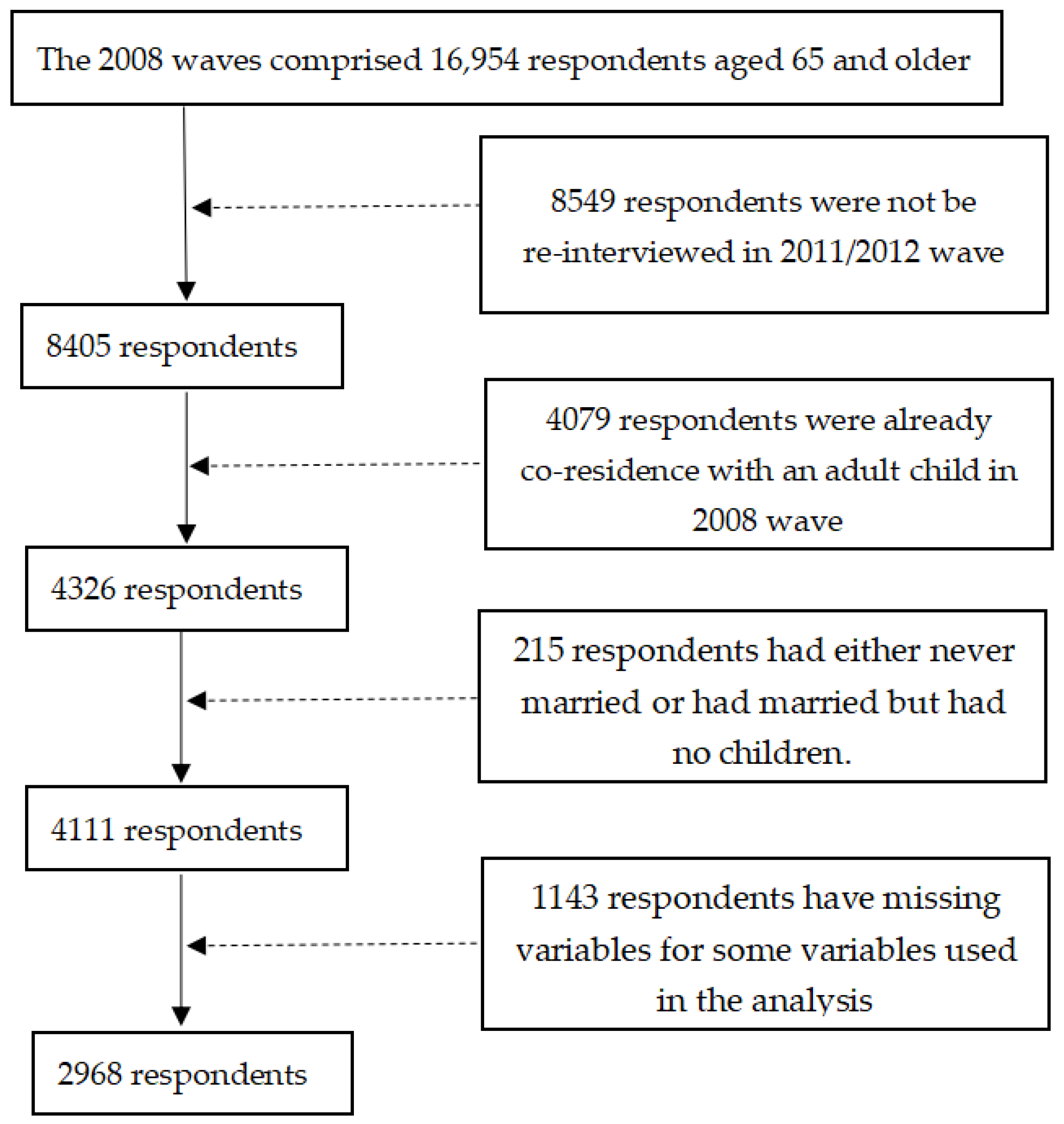
2.1. Data

In our study, the data were derived from the Chinese Longitudinal Healthy Longevity Survey (CLHLS) which was conducted by Peking University for Healthy Aging and Family Studies and the China National Research Center on Aging, with support from Duke University, the United Nations Population Fund (UNFPA), and the Max Planck Institute for Demographic Research [10,22]. The CLHLS collects information on health status and quality of life of the elderly aged 65 and older in 22 provinces of China [16,23]. The total population of the 22 provinces was 1.15 billion in 2010, accounting for about 85 percent of the total population in China. Six waves have taken place: 1998, 2000, 2002, 2005, 2008, and 2011/12, respectively. However, there were only 128 respondents who were followed-up with and re-surveyed in all six waves as many of the earlier respondents were quite old at the time of the first survey and either died by the time of later surveys or were lost to follow-up. In our study, we use the two most recent waves of the CLHLS, namely, 2008 and 2011/12, in order to ensure a high survey follow-up rate. Systematic data quality assessments concerning the reporting age and the reliability, validity, and consistency of series measures showed good quality for CLHLS datasets [10,24,25]. More details about the CLHLS can be found on the website: https://www.icpsr.umich.edu/icpsrweb/NACDA/studies/36179.

The 2008 and 2011/12 waves each comprised 16,954 and 9765 respondents aged 65 and older, respectively. In 2008, 9213 respondents (54.34%) reported co-residence with an adult child, with the majority (7817) co-resident with sons. In 2011/12, 4219 respondents (43.21%) were co-resident with an adult child, and again, the majority (3690) were co-resident with sons. In the 2011/12 survey, 3802 elderly males and 4603 elderly females (for a total of 8405) who were surveyed in 2008 were followed-up with and re-interviewed. The follow-up rate for the two waves was 49.6%.

In our study, among the respondents who were re-interviewed in 201/2012, only respondents who reported that they were not co-residence with an adult child in 2008, n = 4326, were included in order to employ the PSM-DID approach to estimate the causal effects of a transition to co-residence with adult children on the parental subjective well-being. There were 215 respondents who had either never married or did not have children in their marriage. We excluded all of these respondents from the analysis. The resulting sample was composed of 4111 individuals, but because of missing variables for some variables used in the analysis, the analysis sample was thus composed of 2968 elderly parents. Figure 1 shows the flow chart of the selection of the study participants. We compared preserved samples and deleted samples by conducting independent t-tests to test the differences in age between them and by conducting chi-square tests to test the differences in the distribution of gender and marital status. All the test results indicated that there were no significant differences in these demographic features across the two samples. Therefore, it was reasonable for us to delete samples with missing variables for this current analysis.

2.2. Measures

2.2.1. Outcome Variable: The Sustainability of Subjective Well-Being

Well-Being is a broad concept category that includes emotions (such as positive or negative psychological status), personality dispositions (such as extraversion, neuroticism, and self-esteem), depression, loneliness, happiness, and life-satisfaction [26,27,28,29,30]. The CLHLS has consistently included six questions for the elderly concerning self-rated personal status that closely relate to the main aspects of subjective well-being. These questions are as follows:

• How do you rate your life at present?
• Do you always look on the bright side of things?
• Are you as happy now as when you were younger?
• Do you often feel fearful or anxious?
• Do you often feel lonely and isolated?
• Do you feel the older you get the more useless you are?

The responses range from 1 (always or very good) to 5 (never or very bad). Following Chen’s (2008) guidance, we divided subjective well-being into two indices: positive well-being (PWB) (items 1–3); and negative well-being (NWB) (items 4–6) [10]. We rearranged the order of the responses so that for all the items, the 1 value suggested the weakest feeling and the 5 value presented the strongest feeling. We added items 1–3 to create an index of positive well-being, which ranged from 3 to 15, with the higher numbers indicating better well-being. The index of negative well-being was also an aggregation, but of items 4–6, with the resulting values ranging from 3 to 15, with higher values indicating worse well-being.

2.2.2. Treatment Variable: A Transition to Co-Residence with an Adult Child

Co-residence status in the CLHLS was measured by asking respondents about their living arrangements: “How many people are living with you?” and “Who are they?” In our study, the treatment variable was a transition to co-residence with one or more adult children, which is a binary variable assigned a value of one if the respondent did not live with their children in 2008, but changed the living arrangement to co-residence with one or more adult children in 2011/12, n = 677. The treatment variable was zero, this included those who did not live with their adult children in both the 2008 and 2011/12 survey waves, n = 2291.

2.3. Econometric Models

The research question of this study is whether there is a causal effect of transition to co-residence with an adult child on subjective well-being among Chinese old parents. Individual respondents were classified as either experiencing or not experiencing a transition to co-residence with an adult child from non-co-residence between the two survey waves irrespective of the sex of the adult child (e.g., son or daughter). As mentioned in the Background section, in our study, we designed a longitudinal study and employed a PSM-DID approach to overcome the potential selection bias problem in order to estimate unbiased causal effects.

Let $D_{it}$ = 1 denote respondent i who was non-co-resident with an adult child in 2008 but lived with an adult child at a time period t and $D_{it}$ = 0 denote respondent i who still does not live with an adult child at time period t, and let $y_{it+s}^1$ be subjective well-being at time $t+s$, s ≥ 0, following transition. Also denote $y_{it+s}^0$ as the subjective well-being if the respondent had not transferred. The causal effect of a transition to live with an adult child for respondent i at time period $t+s$ is then defined as:

$$y_{it+s}^1-y_{it+s}^0$$

(1)

Fundamentally, for the causal inference, the quantity $y_{it+s}^0$ is unobservable for a respondent that has transferred to co-residence with an adult child (i.e., for which we observe $y_{it+s}^1$) at the time period t + s [31]. In other words, the analysis could be seen as a challenge of the selection bias [31]. Following the literature [20,32,33,34], we defined the average treatment effect of transition (ATT) to co-residence with an adult child on the respondent as:

$$E\left\{y_{t+s}^1-y_{t+s}^0|D_{it}=1\right\}=E\left\{y_{t+s}^1|D_{it}=1\right\}-E\left\{y_{t+s}^0|D_{it}=1\right\}$$

(2)

where the causal inference depends on the counterfactual constructed in Equation (2), which is the outcome of the transferred respondents would have experienced, on average, had they not transferred. This is estimated by the average subjective well-being of the respondent that remained not living with an adult child,$E\left\{y_{it+s}^0|D_{it}=0\right\}$. However, readers should be cautioned that this average causal treatment effect of transferring to co-residence with adult children is only a valid approximation on the condition that there are not any contemporaneous effects that are associated with the treatment variable that are not controlled for [31].

To generate the counterfactual for the transferred respondent, we use propensity score matching (PSM) as proposed by Rosenbaum and Rubin [35]. Using this approach, we estimated the probability (or propensity score) of receiving treatment (transition to co-residence with an adult child) conditional on their characteristics and circumstances in order to reduce the dimensionality problem [35,36,37]. Accordingly, we first estimated the probability of transition using a probit model $P\left(D_{it}=1\right)=F\left(x_{it-1}\right)$, where $x_{it-1}$ constitutes a vector of observed pre-treatment individual characteristics [31,35].

Now let T and C represent the treatment (transition) group and the control group, let $p_i$ denote the predicted probability of transition for respondent i in the treatment (transition) group and let $p_j$ denote the predicted probability of transition for respondent j in the control group. Also, suppose there are $N^T$ numbers of observations in the treatment (transition) group. The average effect of treatment on the transferred (treated) can be estimated as:

$$\mathsf{\mu }=\frac{1}{N^T}{\displaystyle \sum }_{i\in T}(y_i-{\displaystyle \sum }_{j\in C}g\left(p_i,p_j\right)y_i)$$

(3)

where g(.) is a function assigning the weights to be placed on the comparison respondent j while constructing the counterfactual for transferring respondent i [31]. The Gaussian kernel function used in this study is defined as follows:

$$g\left(p_i,p_j\right)=\frac{K\left[\frac{p_i-p_j}{h}\right]}{{{\displaystyle \sum }}_{k\in C}K\left[\frac{p_i-p_k}{h}\right]}$$

(4)

where $\mathrm{K}\left(\mathrm{u}\right)\propto \exp \left(\frac{-{\mathrm{u}}^2}{2}\right)$ is the Gaussian normal function, and h is the bandwidth parameter [31,37].

Since we have longitudinal data, we use a PSM-DID estimator on the matched respondents. This was motivated by studies that argue that standard matching estimators are usually unsatisfactory because of the strong assumption of “selection on observables” [31,38], but in combination with difference-in-differences methodology can have the potential to improve the quality of non-experimental evaluation results significantly [39]. The PSM-DID estimator has the additional advantage of eliminating unobserved time-invariant differences in subjective well-being between co-residence and non-co-residence with an adult child group that standard matching estimators fail to eliminate [31,39].

Following Heckman [19], the PSM-DID estimator is defined as follows. Denote Δy [19] as the difference between the average subjective well-being before and after the transition to co-residence with an adult child. Then the DID estimator can be presented as:

$$\mathsf{\delta }=\frac{1}{N^T}{\displaystyle \sum }_{i\in T}(\Delta y_i-{\displaystyle \sum }_{j\in C}g\left(p_i,p_j\right)\Delta y_i)$$

(5)

We employ variants of this PSM-DID estimator for the empirical analysis below. As commonly done in the literature [19,40,41], bootstrapping (200 repetitions) is used to approximate standard errors. We follow the common convention in the literature of not considering sampling weights in the context of matching [42].

2.4. Matching Covariates

The consideration of “common support” is the foundation to choose covariates for propensity score matching (PSM) between treatment and control groups. According to Heckman et al. (1998, 1999), the implementation of PSM requires a set of variables that are unaffected by treatment which should be included in the matching model [19,20]. In order to satisfy the matching requirement, these variables need either to be fixed over time or to be measured before treated [20]. In terms of the accuracy of matching, Bryson et al. (2002), indicated that over-parameterized models should be avoided, which may lead to the exacerbated common support problem because extraneous variables are included in models, as well as lead to increased variance because too many non-significant variables are used for matching [43]. Therefore, in our study, based on the econometric models employed, and following Rubin et al. [35] and Bryson et al. [43], the probability or “propensity score” of co-residence with an adult child depends on a series of observables, which may illustrate themselves associated with the old parents’ subjective well-being. Following previous studies on the effects of co-residence on elderly parents’ subjective well-being, as well as the available data used in our study, such observables included: first, socio-demographic features such as age, sex, marital status, minority (Han or not); second, social-economic status (SES), such as income, old-age pension, financial distress, years of educated; third, health condition, such as activities of daily living (ADL), disabled, self-rated health; and fourth, additional covariates, such as the number of adult children, and retired status. In this study, we used the “kernel matching estimator (KME)” to match the transferred and non-transferred respondents as done by Heckman et al. and Smith et al. [19,20,39].

Table 1. Summary statistics of the main variables.

Variables.	Mean (SD)/PCT	Min	Max	N
Positive well-being (PWB)_08 (range = 3–15)	13.409 (1.599)	6	15	2968
Negative well-being (NWB)_08 (range = 3–15)	8.48 (2.417)	5	15	2968
Positive well-being (PWB)_11/12 (range = 3–15)	13.314 (1.64)	6	15	2968
Negative well-being (NWB)_11/12 (range = 3–15)	8.697 (2.323)	5	15	2968
Age (years)	78.101 (9.358)	61	110	2968
Female (vs. male)	46.3	0	1	2968
Married (vs. unmarried)	64.2	0	1	2968
Minority (vs. Han)	3.2	0	1	2968
Education (years)	2.648 (3.682)	0	22	2968
Urban (vs. rural)	37.4	0	1	2968
Had activities of daily living disabled (vs. no)	3.5	0	1	2968
Self-rated health (range = 1–5)	3.504 (0.935)	1	5	2968
Log (household income)	8.87 (1.323)	4.382	11.513	2968
Has financial distress (vs. no)	22.6	0	1	2968
Agriculture/fishery occupation (vs. no)	69.3	0	1	2968
Lives in own house (vs. no)	74	0	1	2968
Number of children	4.128 (1.808)	1	13	2968
Has old-age pension (vs. no)	20.07	0	1	2968
Has retired (vs. no)	21.66	0	1	2968

Notes: Means and standard deviations (in parentheses) are provided for the continuous variables and percentages (PCT) are provided for dichotomous variables. The unit of household income is Chinese Yuan per year. Except positive well-being and negative well-being, all of the variables measured were in the 2008 wave.

shows the summary statistics of the main variables used for evaluating matching.

3. Results

In this study, the analysis was divided into 3 sub-parts. To begin with, the PSM-DID approach was implemented in a pooled sample using the two waves of the CLHLS. In order to distinguish any possible macro-wide contextual factors which may lead to heterogeneity in the treatment effects, the sample was decomposed into two Chinese macro blocks, urban and rural China, respectively. Subsequently, considering the traditional culture and elderly living arrangement preference, we were also interested in examining the potential differences in the effect this transition had across the sexes in adult children.

3.1. Pooled Sample

Table 2. Difference-in-differences propensity score matching (PSM-DID) estimates of co-residence with an adult child (pooled sample).

Variable	Sample	Treated	Controls	Difference	S.E.	z-Value	p-Value	Number Treated	Number Control
								677	2291
△PWB	Pre-matching	0.06	−0.14	0.21	0.09	2.35 ***	0.019
	Post-matching	0.07	−0.11	0.17	0.09	1.89 *	0.059
△NWB	Pre-matching	0.01	0.28	−0.27	0.13	−2.01 **	0.045
	Post-matching	0.01	0.17	−0.16	0.14	−1.13	0.259

Note: “Pre-matching” refers to the sample without matching the treatment (transition) group with the control group and “Post-matching” refers to the groups after matching. “Treated” and “Controls” refer to respondents transferring to live with an adult child or not, respectively. ***, **, and * represent significance at the 1%, 5%, and 10% level, respectively. Standard errors were calculated using Bootstrap with 200 replications.

shows the PSM-DID estimates of the effect of co-residence with an adult child with the condition that the sample was pooled. The resulting estimates indicate that transferring to co-residence with an adult child between waves had a significant effect on improving parental positive well-being but did not have a significant effect on negative well-being. The effectiveness of our estimates is proved by the successful balancing test of the treatment and control groups.

Table 3. Balancing test of the treatment and control groups (pooled sample).

Sample	Pseudo R2	LR chi2	p-Value	Mean Bias	Med Bias	B	R
Pre-matching	0.03	104.05	0.00	14.60	15.70	45.0 *	1.11
Post-matching	0.00	0.79	1.00	1.30	1.10	4.80	1.04

Note: The pseudo R² from the probit of treatment on the matching covariates matched the samples before and after matching. The p-values are of the likelihood-ratio test of the joint insignificance of all of the matching covariates. The mean and median bias are the summary indicators of the distribution of the absolute value of bias. B is the absolute standardized difference of the means of the linear index of the propensity score in the treated and matched non-treated group and R is the ratio of treated to matched non-treated variances of the propensity score index. Rubin [44] (2001) recommends that B be less than 25 and that R be between 0.5 and 2 for the samples to be considered sufficiently balanced. An asterisk is displayed next to B and R values that fall outside those limits.

shows that matching reliably eliminates differences in observable and measurable features between the respondents receiving treatment and the controls. It demonstrates the standardized percentage bias of all the covariates used for the propensity score estimation [34]. The lower the standardized percentage bias, the higher the balance (or comparability) between treatment and control groups in terms of observable characteristics [2]. In our study, we are in line with existing empirical studies calculating the standardized percentage bias of all the covariates used for matching, due to the fact that the bias decline for individual covariates may be misleading [2,34,36]. The standardized percentage bias between the treatment and control groups were all under 3%. The pseudo R-squared that approached zero also effectively eliminated any explanatory power of the covariates used in the matching model.

Following Aranda’s [2] (2015) guidance, we graphed the propensity score histogram by treatment status. The “common support” is the foundation on which to choose covariates for propensity score matching between the treatment and control groups. The histograms plotted in Figure 2 shows the goodness of common support between the two groups, which indicates that there was a similar distribution of propensity scores between the two groups. In other words, in our study, we had enough and reasonable cases to serve as comparable counterparts for the treatment group.

3.2. Urban and Rural China

The estimates reported in

Table 4. PSM-DID estimates of co-residence with an adult child (urban and rural).

Variable	Sample	Treated	Controls	Difference	SE	z-Value	p-Value	Number Treated	Number Control
Urban								231	881
△PWB	Pre-matching	−0.14	−0.30	0.16	0.15	1.08	0.280
	Post-matching	−0.14	−0.28	0.14	0.15	0.90	0.368
△NWB	Pre-matching	0.10	0.37	−0.27	0.22	−1.19	0.234
	Post-matching	0.10	0.29	−0.19	0.23	−0.80	0.424
Rural								446	1410
△PWB	Pre-matching	0.17	−0.04	0.21	0.11	1.96 **	0.050
	Post-matching	0.18	−0.01	0.19	0.11	1.69 *	0.091
△NWB	Pre-matching	−0.04	0.23	−0.26	0.17	−1.56	0.119
	Post-matching	−0.04	0.07	−0.10	0.18	−0.59	0.555

Note: “Pre-matching” refers to the sample without matching the treatment (transition) group with the control group and “Post-matching” refers the groups after matching. “Treated” and “Controls” refer to respondents transferring to live with an adult child or not, respectively. ***, **, and * represent significance at the 1%, 5%, and 10% level, respectively. Standard errors were calculated using Bootstrap with 200 replications.

estimate the average impact of the 677 respondents (231 urban respondents and 446 rural respondents) transferring to co-residence with an adult child, and as such, may mask some interesting heterogeneity. Here we ask whether the positive well-being effects were the same in urban and rural parts of China under consideration. For the urban parts of China, 231 respondents transferring to co-residence with an adult child were observed in our sample. The estimates presented in Table 4 shed some light on this issue.

Table 4 reports that transferring to co-residence with an adult child between waves had a significant effect on improving parental positive well-being in rural China, but not in urban China. However, the transition did not have a significant effect on parental negative well-being both in urban and rural China. The balancing tests that followed (

Table 5. Balancing tests of the treatment and control groups (pooled sample).

Sample	Pseudo R2	LR chi2	p-Value	MeanBias	MedBias	B	R
Urban
Pre-matching	0.04	43.39	0.00	14.30	13.20	49.3 *	1.08
Post-matching	0.00	0.43	1.00	1.70	1.30	6.10	1.18
Rural
Pre-matching	0.04	71.51	0.00	15.70	12.70	46.0 *	1.18
Post-matching	0.00	0.42	1.00	1.40	1.20	4.30	1.20

Note: Pseudo R² from the probit of the treatment on the matching covariates matched samples before and after matching. The p-values are of the likelihood-ratio test of the joint insignificance of all of the matching covariates. The mean and median bias are the summary indicators of the distribution of the absolute value of bias. B is the absolute standardized difference of the means of the linear index of the propensity score in the treated and matched non-treated group and R is the ratio of treated to matched non-treated variances of the propensity score index. Rubin [44] (2001) recommends that B be less than 25 and that R be between 0.5 and 2 for the samples to be considered sufficiently balanced. An asterisk is displayed next to B and R values that fall outside those limits.

and Figure 3; Figure 4) assert the overall validity of our findings.

3.3. Son versus Daughter

Given the difference in effects between urban and rural China, it was also interesting to see if there was a difference in effect when co-residence was with a son or daughter, as that difference is stressed with the Chinese cultural tradition of Confucianism. One common Chinese proverb stresses the importance of “raising sons for old age” [45].

More respondents transferred to co-residence with a son than a daughter over the time period analyzed. In the 2011/2012 wave, 555 parents transferred to co-residence with a son and 122 parents transferred to co-residence with a daughter. The PSM-DID estimates reported in

Table 6. PSM-DID estimates of co-residence with an adult child (son and daughter).

Variable	Sample	Treated	Controls	Difference	S.E.	z-Value	p-Value	Number Treated	Number Control
Son								555	2289
△PWB	Pre-matching	0.08	−0.14	0.22	0.10	2.28 ***	0.023
	Post-matching	0.08	−0.11	0.18	0.10	1.89 *	0.059
△NWB	Pre-matching	0.07	0.28	−0.21	0.14	−1.42	0.156
	Post-matching	0.07	0.16	−0.09	0.15	−0.62	0.535
Daughter								122	2722
△PWB	Pre-matching	0.03	−0.14	0.17	0.20	0.85	0.395
	Post-matching	0.03	−0.13	0.16	0.20	0.81	0.418
△NWB	Pre-matching	−0.42	0.28	−0.70	0.30	−2.32 ***	0.020
	Post-matching	−0.42	0.21	−0.63	0.31	−2.05 ***	0.040

Note: “Pre-matching” refers to the sample without matching the treatment (transition) group with the control group and “Post-matching” refers the groups after matching. “Treated” and “Controls” refer to respondents transferring to live with an adult child or not, respectively. ***, **, and * represent significance at the 1%, 5%, and 10% level, respectively. Standard errors were calculated using Bootstrap with 200 replications.

revealed substantial differences between co-residence with a son and a daughter. A remarkable effect emerged: transferring to co-residence with a son significantly improved parental positive well-being, while no significant effect of co-residence with a son on negative well-being was observed. On the other hand, respondents transferring to co-residence with a daughter had significantly lower negative well-being, while no significant effect of co-residence with a daughter was observed on positive well-being.

According to the balancing tests (

Table 7. Balancing test of the treatment and control groups (son and daughter).

Sample	Pseudo R2	LR chi2	p-Value	MeanBias	MedBias	B	R
Son
Pre-matching	0.04	117.86	0.00	17.90	20.10	52.3 *	0.95
Post-matching	0.00	0.92	1.00	1.70	0.90	5.80	1.05
Daughter
Pre-matching	0.04	33.02	0.00	14.50	8.50	58.2 *	1.04
Post-matching	0.02	6.16	0.94	8.70	5.30	34.2 *	0.93

Note: Pseudo R² from the probit of the treatment on the matching covariates matched samples before and after matching. The p-values are of the likelihood-ratio test of the joint insignificance of all of the matching covariates. The mean and median bias are the summary indicators of the distribution of the absolute value of bias. B is the absolute standardized difference of the means of the linear index of the propensity score in the treated and matched non-treated group and R is the ratio of treated to matched non-treated variances of the propensity score index. Rubin [44] (2001) recommends that B be less than 25 and that R be between 0.5 and 2 for the samples to be considered sufficiently balanced. An asterisk is displayed next to B and R values that fall outside those limits.

and Figure 5 and Figure 6), caution is advised when interpreting the effect of transferring to co-residence with a daughter, given the relatively small post-matching bias reduction (37.6%). The comparability between treatment group and control group may be challenged in this sub-analysis due to the small sample size of that transition to co-residence with daughter. In order to check the sensitivity caused by the possible small sample bias, we undertook robustness tests for our model.

3.4. Robustness Tests

In this study, we used both nearest-neighbor matching and radius matching as robustness tests to reexamine the model [46]. Focusing on the pooled sample in Panel A of

Table 8. Estimation of effects using Nearest neighbor matching, Radius matching, Kernel matching.

Variable	A.Pooled			B.Urban			C.Rural			D.Son			E.Daughter
	ATT	z-Value	p-Value	ATT	z-Value	p-Value	ATT	z-Value	p-Value	ATT	z-Value	p-Value	ATT	z-Value	p-Value
Nearest-neighbor matching
△PWB	0.21	2.08 **	0.038	0.28	1.61	0.108	0.2	1.59	0.112	0.13	1.17	0.242	0.06	0.24	0.810
△NWB	−0.12	−0.75	0.453	−0.42	−1.57	0.117	0.01	0.05	0.960	−0.23	−1.31	0.190	−0.66	−1.841 *	0.066
Radius matching
△PWB	0.16	1.703 *	0.089	0.15	0.98	0.327	0.21	1.807 *	0.071	0.18	1.86 *	0.063	0.14	0.71	0.478
△NWB	−0.15	−1.06	0.289	−0.18	−0.76	0.447	−0.08	−0.45	0.653	−0.08	−0.53	0.596	−0.54	−1.724 *	0.085
Kernel matching
△PWB	0.17	1.894 *	0.058	0.14	0.9	0.368	0.19	1.69 *	0.091	0.18	1.89 *	0.059	0.16	0.81	0.418
△NWB	−0.16	−1.13	0.259	−0.19	−0.8	0.424	−0.1	−0.59	0.555	−0.1	−0.62	0.535	−0.63	−2.047 **	0.041

Note: ATT means average treatment effect on the treated. ***, **, and * represent significance at the 1%, 5%, and 10% level, respectively. Standard errors were calculated using Bootstrap with 200 replications.

, we found similar results by the neighbor matching and radius matching methods as those in Table 8. Hence, the resulting estimates confirm the robustness of our identification strategy, as conventional levels of statistical significance were reached irrespective of the method used. Focusing on the subgroups in Panels B–E, we also identified similar patterns when using these two approaches. Thus, the robustness of the results is demonstrated.

4. Discussion

The non-parametric PSM-DID approach was designed by Heckman et al. (1998, 1999, 2005) to overcome the problem of selection bias and to estimate unbiased causal effects [18,19,20]. In this study, we employed the PSM-DID approach to assess the causal effects of a transition to co-residence with adult children on parental well-being. Our study contributes to the international literature through its application of the PSM-DID methods to obtain unbiased estimates of the relationship between living arrangements and the well-being of elderly Chinese citizens in both urban and rural areas, as well as infer causal effects using a longitudinal design.

In the pooled sample, transferring to co-residence with an adult child had a significant effect on positive parental well-being, which is in line with some previous literature [11,16]. However, we found little statistically significant evidence of a casual effect of co-residence with adult children on negative parental well-being. These findings represent a challenge to some studies that indicated that co-residence with adult children reduced parental life-satisfaction and well-being [47,48]. One potential explanation for these findings is the role of Confucianism and the tradition of filial piety in the Chinese context, wherein co-residence with adult children may still be the preferred living arrangement for some Chinese elderly parents [49]. If the transition to co-residence with adult children conforms to the parents’ preferred living arrangements, then this form of co-residence will tend to have a positive effect on parental subjective well-being.

Given differences in the socio-economic and development status of rural and urban residents of China, the study assessed whether there were also differences in the causal effects of a transition to co-residence with adult children on parents’ well-being across these two regions. Indeed, some interesting and thought-provoking results emerged: compared to the pooled sample results, in rural China, co-residence with adult children significantly increased positive well-being, but it did not significantly influence negative well-being both in rural and urban China. One possible reason for this finding was alluded to in some previous studies. There has been a significant difference in the development of old-age insurance and social services for old adults between rural and urban regions that has differentially influenced the extent to which the elderly are dependent on their adult children in the two areas [50]. Moreover, the sense of “filial piety” and altruism that encouraged adult children to support their old parents still has a profound impact on the choice of living arrangements for rural communities [49,51]. For example, it is a shame for many rural older adults to live alone or live in a nursing home without daily care from their adult children.

Inspired by the observed differences across rural and urban areas, we also examined the effects of co-residence on parental subjective well-being by assessing the gender of the adult children. According to the PSM-DID estimates, we found that co-residence with a son significantly increased parental positive subjective well-being, and negative well-being fell if co-residence was with an adult daughter. In this current study, the estimation outcomes seem contradictory compared with some previous studies, which claimed that the conflicts and unhappy relationship between a daughter-in-law and parents-in-law may account for declines in parental well-being if co-residence was with a daughter-in-law [11,52,53]. However, our findings imply that, consistent with traditions to value “bringing up sons to support parents in their old age”, co-residence with an adult son was preferred among Chinese elderly parents and was associated with higher performance in parental well-being.

In this current study, our findings are reliable based on these following strengths. On one hand, we put our research question into a longitudinal design, which aimed to capture the differences in parental subjective well-being performance between the pre-transition and post-transition of co-residence with adult children. On the other hand, we employed a PSM-DID approach with the advantage to address the selection bias problem in the archive investigations to obtain an unbiased causal inference. Furthermore, our study was embedded in the Chinese social and traditional context, and we examined the potential differences in the effect of this transition due to the sex of the adult children and urban–rural status.

There are some limitations with our study. First, the sample size was relatively small. This was because many respondents died between the two study waves. However, we applied bootstrap methods to deal with the potential for small sample bias. Second, the accuracy of matching may have been influenced by the unobserved characteristics of respondents. Third, some characteristics of adult children that may influenced the decision to co-reside were not available in the CLHLS dataset. Fourth, some studies have reported that adult children who move back to the parental home due to the presence of economic stress may reduce parents’ well-being [2,6]. However, our study did not distinguish the direction of the co-residence transition, because the question asked in the CLHLS did not confirm whether the adult children moved to co-reside with the parents or whether the parents moved to co-reside with the adult children.

5. Conclusions

This study assessed the effects of a transition to co-residence with adult children on parental subjective well-being sustainability. In order to address the ambiguity in the international literature, potentially resulting from various statistical challenges, we applied the PSM-DID approach within the context of a longitudinal design that controlled for potential selection bias. Our key finding was that co-residence with adult children significantly improved the sustainability of parental PWB. This may imply that, in the Chinese context, old adults’ living arrangements and its change was associated with their well-being. Moreover, in our study, we found that a transition to co-residence with adult children causally improved parental well-being. Our findings provide insight for policy and decision-making concerning efforts to facilitate the strengthening of family support. Our findings suggest that by strengthening opportunities for co-residence, the well-being of older Chinese residents will be improved.

References

1. Brackbill, Y.; Kitch, D. Intergenerational relationships: A social exchange perspective on joint living arrangements among the elderly and their relatives. J. Aging Stud. 1991, 5, 77–97. [Google Scholar] [CrossRef]
2. Aranda, L. Doubling up: A gift or a shame? Intergenerational households and parental depression of older Europeans. Soc. Sci. Med. 2015, 134, 12–22. [Google Scholar]
3. Courtin, E.; Avendano, M. Under one roof: The effect of co-residing with adult children on depression in later life. Soc. Sci. Med. 2016, 168, 140–149. [Google Scholar] [CrossRef]
4. Ferguson, L.E. Examining Generational and Gender Differences in Parent-Young Adult Child Relationships During Co-Residence. Master’s Thesis, Portland State Uniersity, Portland, OR, USA, October 2016. [Google Scholar]
5. Taniguchi, H.; Kaufman, G. Filial Norms, Co-Residence, and Intergenerational Exchange in Japan. Soc. Sci. Q. 2017, 98, 1518–1535. [Google Scholar] [CrossRef]
6. Tosi, M.; Grundy, E. Returns home by children and changes in parents’ well-being in Europe. Soc. Sci. Med. 2018, 200, 99–106. [Google Scholar] [CrossRef] [PubMed]
7. Warner, C.; Houle, J.N. Precocious life course transitions, exits from, and returns to the parental home. Adv. Life Course Res. 2018, 35, 1–10. [Google Scholar] [CrossRef]
8. Zhou, Z.; Mao, F.; Ma, J.; Hao, F.; Qian, Z.; Elder, K.; Turner, J.S.; Fang, Y. A Longitudinal Analysis of the Association Between Living Arrangements and Health Among Older Adults in China. Res. Aging 2018, 40, 72–97. [Google Scholar] [CrossRef] [PubMed]
9. Muennig, P.; Jiao, B.; Singer, E. Living with parents or grandparents increases social capital and survival: 2014 General Social Survey-National Death Index. SSM Popul. Health 2018, 4, 71–75. [Google Scholar] [CrossRef]
10. Chen, F.; Short, S.E. Household Context and Subjective Well-Being Among the Oldest Old in China. J. Fam. Issues 2008, 29, 1379–1403. [Google Scholar] [CrossRef]
11. Zhang, L. Living Arrangements and Subjective Well-Being among the Chinese Elderly. Open J. Soc. Sci. 2015, 3, 150–161. [Google Scholar] [CrossRef]
12. Lei, X.; Strauss, J.; Tian, M.; Zhao, Y. Living arrangements of the elderly in china: evidence from charls. Iza Discussion Papers 2011, 8. [Google Scholar] [CrossRef]
13. Lei, X.; Strauss, J.; Tian, M.; Zhao, Y. Living arrangements of the elderly in China: Evidence from the CHARLS national baseline. Chin. Econ. J. 2015, 8, 191–214. [Google Scholar] [CrossRef]
14. Yi, Z.; Wang, Z. Dynamics of family and elderly living arrangements in China: New lessons learned from the 2000 Census. Chin. Rev. 2003, 3, 95–119. [Google Scholar]
15. Zhou, Y.; Zhou, L.; Fu, C.; Wang, Y.; Liu, Q.; Wu, H.; Zhang, R.; Zheng, L. Socio-economic factors related with the subjective well-being of the rural elderly people living independently in China. Int. J. Equity Health 2015, 14, 5. [Google Scholar] [CrossRef]
16. Wang, J.; Chen, T.; Han, B. Does co-residence with adult children associate with better psychological well-being among the oldest old in China? Aging Ment. Health 2014, 18, 232–239. [Google Scholar] [CrossRef]
17. Heckman, J.J. Sample Selection Bias as a Specification Error. Econometrica 1979, 47, 153–161. [Google Scholar] [CrossRef]
18. Wang, M.; Zhan, Y.; Liu, S.; Shultz, K.S. Antecedents of bridge employment: A longitudinal investigation. J. Appl. Psychol. 2008, 93, 818–830. [Google Scholar] [CrossRef]
19. Heckman, J.J.; Ichimura, H.; Todd, P.E. Matching as an econometric evaluation estimator: Evidence from evaluating a job training programme. Rev. Econ. Stud. 1998, 65, 261–294. [Google Scholar] [CrossRef]
20. Heckman, J.J.; Lalonde, R.J.; Smith, J.A. The Economics and Econometrics of Active Labor Market Programs. In Handbook of Labor Economics; Elsevier: Amsterdam, The Netherlands, 1999; Volume 3, pp. 1865–2097. [Google Scholar]
21. Heckman, J.J.; Vytlacil, E. Structural Equations, Treatment Effects, and Econometric Policy Evaluation 1. Econometrica 2005, 73, 669–738. [Google Scholar] [CrossRef]
22. Zeng, Y.; Feng, Q.; Hesketh, T.; Christensen, K.; Vaupel, J.W. Survival, disabilities in activities of daily living, and physical and cognitive functioning among the oldest-old in China: A cohort study. Lancet 2017, 389, 1619–1629. [Google Scholar] [CrossRef]
23. Zeng, Y.; Vaupel, J.; Xiao, Z.; Liu, Y.; Zhang, C. Chinese Longitudinal Healthy Longevity Survey (CLHLS), 1998–2012; ICPSR36179-v1; Inter-University Consortium for Political and Social Research: Ann Arbor, MI, USA, 2015; Volume 1. [Google Scholar] [CrossRef]
24. Zeng, Y.; Poston, D.L., Jr.; Ashbaugh Vlosky, D.; Gu, D. Healthy Longevity in China; Springer: Berlin, Germany, 2008; pp. 312–313. [Google Scholar]
25. Zeng, Y.I.; Wang, Z.; Jiang, L.; Gu, D. Future trend of family households and elderly living arrangement in China. Genus 2008, 64, 9–36. [Google Scholar]
26. Diener, E. Assessing subjective well-being: Progress and opportunities. Soc. Indic. Res. 1994, 31, 103–157. [Google Scholar] [CrossRef]
27. Diener, E.; Suh, E.M.; Lucas, R.E.; Smith, H.L. Subjective Well-Being: Three Decades of Progress. Psychol. Bull. 1999, 125, 276–302. [Google Scholar] [CrossRef]
28. Diener, E.; Oishi, S.; Lucas, R.E. Personality, culture, and subjective well-being: emotional and cognitive evaluations of life. Ann. Rev. Psychol. 2003, 54, 403–425. [Google Scholar] [CrossRef]
29. Hayes, N.; Joseph, S. Big 5 correlates of three measures of subjective well-being. Personal. Individ. Differ. 2003, 34, 723–727. [Google Scholar] [CrossRef]
30. Diener, E.; Larsen, R.J.; Emmons, R.A. Person × situation interactions: Choice of situations and congruence response models. J. Personal. Soc. Psychol. 1984, 47, 580–592. [Google Scholar] [CrossRef]
31. Girma, S.; Görg, H. Evaluating the foreign ownership wage premium using a difference-in-differences matching approach. J. Int. Econ. 2007, 72, 97–112. [Google Scholar] [CrossRef]
32. Dehejia, R.H.; Wahba, S. Propensity Score-Matching Methods for Nonexperimental Causal Studies. Rev. Econ. Stat. 2002, 84, 151–161. [Google Scholar] [CrossRef]
33. Dehejia, R.H. Program evaluation as a decision problem. J. Econ. 2005, 125, 141–173. [Google Scholar] [CrossRef]
34. Rosenbaum, P.R.; Rubin, D.B. The central role of the propensity score in observational studies for causal effects. Biometrika 1983, 70, 41–55. [Google Scholar] [CrossRef]
35. Rubin, D.B.; Thomas, N. Combining propensity score matching with additional adjustments for prognostic covariates. J. Am. Stat. Assoc. 2000, 95, 573–585. [Google Scholar] [CrossRef]
36. Rosenbaum, P.R.; Rubin, D.B. Constructing a Control Group Using Multivariate Matched Sampling Methods That Incorporate the Propensity Score. Am. Stat. 2012, 39, 33–38. [Google Scholar]
37. Babaud, J.; Witkin, A.P.; Baudin, M.; Duda, R.O. Uniqueness of the Gaussian kernel for scale-space filtering. IEEE Trans. Pattern Anal. Mach. Intell. 1986, 1, 26–33. [Google Scholar] [CrossRef]
38. Blundell, R.; Dias, M.C. Evaluation methods for non-experimental data. Fisc. Stud. 2000, 21, 427–468. [Google Scholar] [CrossRef]
39. Smith, J.A.; Todd, P.E. Does matching overcome LaLonde’s critique of nonexperimental estimators? J. Econom. 2005, 125, 305–353. [Google Scholar] [CrossRef]
40. Lechner, M. The Estimation of causal effects by difference-in-difference methodsestimation of spatial panels. Found. Trends Econom. 2010, 4, 165–224. [Google Scholar] [CrossRef]
41. Dan, A.B.; Smith, J.A. How robust is the evidence on the effects of college quality? Evidence from matching. J. Econom. 2004, 121, 99–124. [Google Scholar]
42. Leuven, E.; Sianesi, B. PSMATCH2: Stata Module to Perform Full Mahalanobis and Propensity Score Matching, Common Support Graphing, and Covariate Imbalance Testing, 2018. Available online: https://ideas.repec.org/c/boc/bocode/s432001.html (accessed on 3 February 2018).
43. Bryson, A.; Dorsett, R.; Purdon, S. The Use of Propensity Score Matching in the Evaluation of Active Labour Market Policies. Lse Research Online Documents on Economics, 2002. Available online: http://eprints.lse.ac.uk/4993/ (accessed on 3 February 2018).
44. Rubin, D.B. Using Propensity Scores to Help Design Observational Studies: Application to the Tobacco Litigation. Health Serv. Outcomes Res. Methodol. 2001, 2, 169–188. [Google Scholar] [CrossRef]
45. Zhang, Y.; Xiao, R. The relationship among raising sons for old age, more sons more happiness and pension tendency of rural elderly. Chongqing Soc. Sci. 2016, 3, 59–67. [Google Scholar]
46. Lian, Y.; Su, Z.; Gu, Y. Evaluating the effects of equity incentives using PSM: Evidence from China. Front. Bus. Res. Chin. 2011, 5, 266–290. [Google Scholar] [CrossRef]
47. Ren, Q.; Treiman, D.J. Living arrangements of the elderly in china and consequences for their emotional well-being. Chin. Soc. Rev. 2015, 47, 255–286. [Google Scholar] [CrossRef]
48. Jin, Q.; Pearce, P.; Hu, H. The study on the satisfaction of the elderly people living with their children. Soc. Indic. Res. 2017, 140, 1159–1172. [Google Scholar] [CrossRef]
49. Sereny, M.D. Family Ties, Economic Resources, and the Well-Being of Older Adults Across Communities in China. Ph.D. Thesis, Duke University, Durham, NC, USA, 2013. [Google Scholar]
50. Cheng, L.; Liu, H.; Zhang, Y.; Zhang, Z. The heterogeneous impact of pension income on elderly living arrangements: evidence from China’s new rural pension scheme. J. Popul. Econ. 2017, 31, 155–192. [Google Scholar] [CrossRef]
51. Frankenberg, E.; Lillard, L.; Willis, R.J. Patterns of intergenerational transfers in Southeast Asia. J. Marriage Fam. 2002, 64, 627–641. [Google Scholar] [CrossRef]
52. Kim, H.S.; Sherman, D.K.; Ko, D.; Taylor, S.E. Pursuit of comfort and pursuit of harmony: Culture, relationships, and social support seeking. Personal. Soc. Psychol. Bull. 2006, 32, 595–607. [Google Scholar] [CrossRef]
53. Ikels, C. The impact of housing policy on China’s urban elderly. Urban Anthropol. Stud. Cult. Syst. World Econ. Dev. 2004, 33, 321–355. [Google Scholar]
Figure 1. Low chart of the selection of the study participants.
Sustainability 11 02090 g001
Figure 2. Propensity score histogram for the treatment and control groups (pooled sample). Note: The graph of the propensity score histogram by treatment status was done by commander “psgraph” in Stata 14. “On support” means the propensity score of the observation on the region of the common support or overlap between the treatment and control groups. “Off support” means the observation off the common support. The propensity score was obtained using matching covariates.
Sustainability 11 02090 g002
Figure 3. Propensity score histogram for the treatment and control groups (urban). Note: The graph of the propensity score histogram by treatment status was done by commander “psgraph” in Stata 14. “On support” means the propensity score of the observation on the region of the common support or overlap between the treatment and control groups. “Off support” means the observation off the common support. The propensity score was obtained using matching covariates.
Sustainability 11 02090 g003
Figure 4. Propensity score histogram for the treatment and control groups (rural). Note: The graph of the propensity score histogram by treatment status was done by commander “psgraph” in Stata 14. “On support” means the propensity score of the observation on the region of the common support or overlap between the treatment and control groups. “Off support” means the observation off the common support. The propensity score was obtained using matching covariates.
Sustainability 11 02090 g004
Figure 5. Propensity score histogram for the treatment and control groups (son). Note: Graph the propensity score histogram by treatment status by commander “psgraph” in Stata 14; “On support” means the propensity score of the observation on the region of the common support or overlap between treatment and control groups. “Off support” means the observation off the common support; The propensity score obtained using matching covariates.
Sustainability 11 02090 g005
Figure 6. Propensity score histogram for the treatment and control groups (daughter). Note: The graph of the propensity score histogram by treatment status was done by commander “psgraph” in Stata 14. “On support” means the propensity score of the observation on the region of the common support or overlap between the treatment and control groups. “Off support” means the observation off the common support. The propensity score was obtained using matching covariates.
Sustainability 11 02090 g006