Prioritizing Green Spaces for Biodiversity Conservation in Beijing Based on Habitat Network Connectivity

Abstract

Rapid urbanization results in changes in land use, biogeochemical cycles, climate, hydrosystems, and biodiversity. Policy-makers have formulated ecological protection measures to facilitate sustainable development. However, traditional conservation planning mainly focuses on protecting specific green spaces, with limited consideration of the connectivity among green spaces from a habitat network perspective. Using citizen science data and occupancy modelling, we predicted habitat suitability, built habitat networks and identified key habitat patches based on their contribution to the functional connectivity of the habitat network for three focal water, forest, and open-habitat bird species. Based on the habitat requirement, small waterbodies and intermediate forest and open-habitat cover facilitate preserving water, forest and open-habitat birds. In regards to the network analysis, we found that key habitat patches with a high conservation priority were generally characterized by a relatively large patch size and/or located at critical positions in the habitat network (at central positions in the habitat network, or near large patches). We suggest that key habitat patches in restricted built-up areas are converted to protected areas or are kept as cropland under future urban planning. We emphasize the usefulness of the focal species concept in urban biodiversity conservation. Our study offers conservation recommendations from a habitat network perspective for urban planners to safeguard urban biodiversity and ecosystem health.

1. Introduction

The world has experienced widespread urbanization, especially since 1950, with around 55% of the current human population living in urban areas [1]. In China, the urbanization rate was 18% in 1978, and reached 56% by 2015, due to the program of economic reform starting in 1978 [2]. Rapid urbanization results in changes in land use, biogeochemical cycles, climate, hydrosystems, and biodiversity, from local to regional scales [3]. Furthermore, the conversion of urban green spaces and suburban land into built-up land results in a fragmented landscape and isolated habitat patches for flora and fauna [4]. Such changes negatively affect species’ survival, leading to both functional homogenization of bird communities [5] and a reduction of species richness in biotic communities [3,6]. This alters ecosystem structure and function, and ultimately influences ecosystem services and human well-being [7].

To both conserve urban biodiversity and achieve sustainable development, action is needed to restore the fragmented natural environment into an integrated system [8]. As space is limited in urban areas, large-scale restoration is impractical [9]. In the past, the island biogeography theory was primarily used to target areas for protection [10]. It suggests targeting bigger reserves, positioned closer to each other and approaching a circular shape, and connected by habitat corridors [11,12]. In reality, due to the constrains in cost and land use history, conservation planners can often only protect large reserves or a series of smaller ones that possess a relatively high biodiversity [13]. In this case, how critical these reserves in facilitating the overall habitat connectivity is not clear. To account for all potential habitat patches, the concept of habitat network connectivity was developed to evaluate the overall landscape conditions [8,14,15,16].

Habitat network connectivity reflects the functional connection among habitat patches across the landscape, so the degree to which the landscape allows or impedes the movement of organisms among habitat patches [14]. Habitat network connectivity reflects the degree of habitat availability for an organism located at any specific point on the landscape. Increased habitat network connectivity positively affects species’ abundance [17], persistence and diversity [18]. The loss of a specific habitat patch might influence network connectivity in different ways [19] and crucial habitat patches could be identified based on their contribution to overall connectivity and allocated conservation priority [20].

Habitat network connectivity analysis has been used before to guide both rural and urban conservation. For example, Kang et al. [21] examined how local habitat patch area, vegetation complexity, human disturbance, and habitat connectivity influenced the diversity of forest bird communities in forest patches embedded in an urbanized landscape and confirmed the positive influence of high habitat connectivity on the survival and diversity of forest birds. Fajardo et al. [22] combined habitat suitability and connectivity analysis to reveal gaps in conservation for mammal, bird, amphibian, reptile, butterfly, and plant species in Peru. Gao et al. [23] constructed habitat networks based on habitat quality assessment by the InVEST (Integrated Valuation of Ecosystem Services and Trade-offs) model, focusing on ecosystem services for mammals, and identified important areas for conservation priority in Changzhou, China. Dondina et al. [24] proposed a method to identify an ecological network based on species specific perception of the landscape [25] and to prioritize areas for implementing or restoring corridors to enhance landscape connectivity [26].

Most urban studies simply consider green spaces to represent habitat patches for animals in general, whereas few studies actually quantify the suitability of these green spaces for specific species [27,28]. The main limitation in habitat suitability estimation is that observation data of target species are frequently unavailable, or collected under imperfect detection (species go undetected by the observer but actually occur there) [29]. Big citizen science data are considered a valuable resource to model species’ distribution [30]. In combination with occupancy modelling, which specifically takes sampling bias into account [31], suitable habitat could be accurately mapped [30,32], providing the foundation for a habitat network. Birds are sensitive to habitat quality and are considered suitable bio-indicators for environmental quality and ecosystem health [33]. For example, water birds are often used as bio-indicators for the health of wetland ecosystems [34,35]. Furthermore, birds are easy to observe in most habitat within urban, suburban and rural landscapes.

Beijing municipality experiences rapid urbanization [36]. The Beijing Urban Master Plan (2016–2035), released in September 2017, delineates the boundary of ecological control areas (protected areas). The remaining land surface is classified as restricted built-up areas and intense built-up areas (Figure 1b). Restricted built-up areas are transition areas, which could be converted into either intense built-up areas or ecological control areas by the end of 2035. Green spaces located in areas of restricted built-up are potentially important for conserving biodiversity for conserving bird [37] diversity and that of several other taxa of vertebrates [38,39] and invertebrates [40,41]. It is vital to identify those green spaces that are crucial for habitat network connectivity, to prevent them from being transformed into intense built-up areas. Using Beijing as an example, this study aims to (1) construct habitat networks of three focal species considered representative for water, forest and open-habitat bird communities, based on citizen science data and occupancy modelling, and (2) prioritize habitat patches for conservation based on their contribution to habitat network connectivity.

2. Materials and Methods

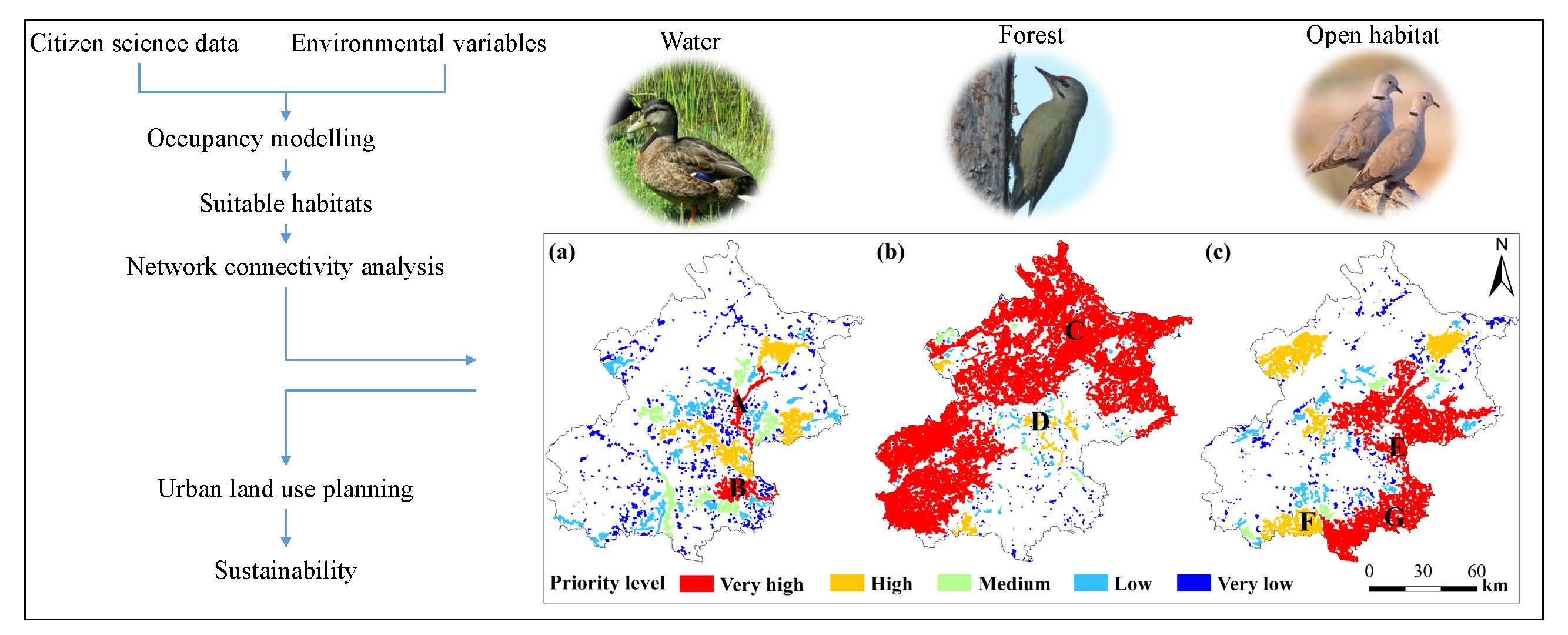
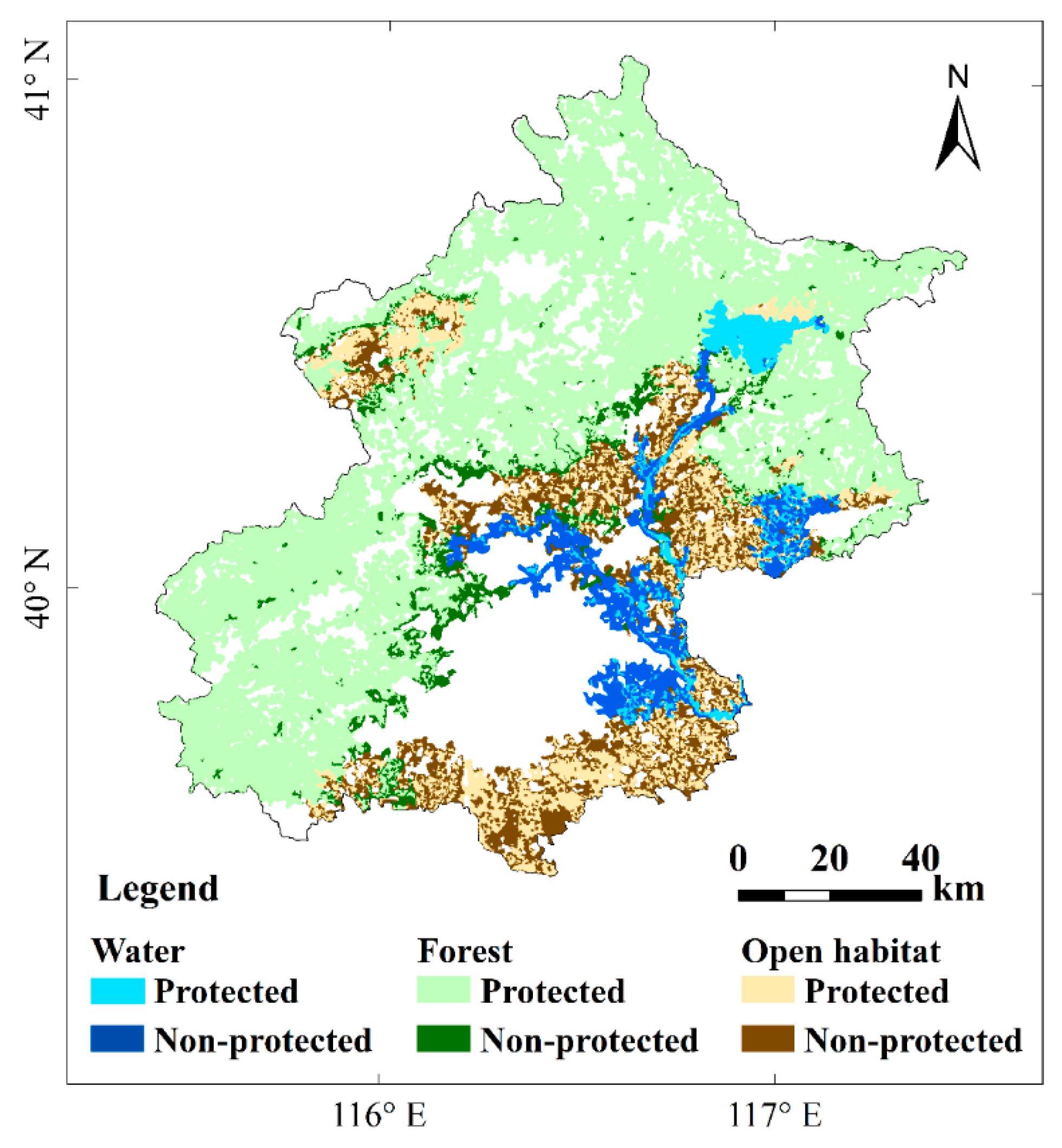
2.1. Study Area

Beijing is the capital of China, located in the northern part of the North China Plain (39.4°–41.6° N, 115.7°–117.4° E). Beijing municipality covers 16,808 km² and is characterized by distinct landforms, with mountains located in the northwest and plains located in the southeast (Figure 1a). Mountainous area occupies 61.3% of the municipality and is mainly covered with shrubs and trees. The plain covers the remaining 38.7% and is the main area of urban sprawl [42]. The diverse habitat types produced by the combination of landforms support a rich flora and fauna.

2.2. Bird Data and Focal Species Selection

We downloaded bird observation data from the online gateway China Bird Report Center [43], which as metadata includes the species name, observation time, observation site (place name), species count and the username of the observer. We used relatively recent bird observation records for the 2008—2017 decade. We checked the location of each site based on 2015 Google Earth images and obtained the longitude and latitude of the site center following Li et al. [44].

In total, we obtained observation records for 545 bird species at 150 observation sites, including 81 resident, 179 migratory, 91 breeding, 42 wintering and 152 vagrant bird species [45,46]. We focus on resident birds (14 generalists were excluded) with observation records available throughout the year. We then categorized them into water, forest, and open-habitat bird communities, according to their main habitat requirement [45,46]. Water, forest, and open-habitat birds refer to groups of birds that use water, forest, or open areas (such as farmland and grassland), as their main habitat.

The focal species concept is defined as a species or group of species for which their spatial and functional requirements encapsulate those of many other species [47]. For each of the three bird communities we chose one focal species. We used three criteria for selection: the habitat “barycenter” $B_s$ [48], the observation frequency (OF), and the variance of $B_s$ confidence intervals (VBCI). Habitat “barycenter” $B_s$ quantifies the habitat requirement (here referring to the habitat coverage) of a species. VBCI quantifies the variance of the habitat requirement (difference between the upper and lower limit of 95% confidence intervals of habitat coverage at each site). Species with a relatively narrow variance is more selective. Observation frequency (OF) was calculated as the number of sites in which a species was observed, divided by the total number of observation sites. It indicates the sample size of the presence data for each species.

Habitat “barycenter” $B_s$ is calculated by Equation (1):

$$B_s=\frac{{\displaystyle \sum }{n}_i\times x_i}{N}$$

(1)

where $B_s$ is the habitat barycenter of species $s$, $n_i$ is the number of individuals at the $i$th observation site, $x_i$ is the value of environmental variables (water, forest, or open-habitat coverage) at the $i$th observation site and $N$ is the total number of individuals recorded at all sites.

Since the median area of the observation sites is 1.2 km², which equals the size of a 600 m-radius buffer, we used a 600 m-radius buffer from the center location of the observation site to calculate the habitat composition for each observation site, $B_s$ and VBCI. All analyses were carried out using the raster package version 2.8-19 (University of California Davis, Davis, CA, USA) [49] in the R statistical software version 3.5.0 (R Foundation for Statistical Computing, Vienna, Austria) [50].

Species with both high $B_s$ (>0.3) [48] and OF (>0.2, equals to being observed at more than 30 sites) values were pre-selected as candidate focal species (

Table A1. Summary of 14 studied resident water bird species observed from 2008–2017 in Beijing municipality. $B_s$: the weighted mean of water coverage at all site of presence; OF: observation frequency calculated as the number of sites in which a species was observed, divided by the total number of observation sites; LCI: lower limit of 95% confidence interval for the water coverage at all site of presence; UCL: upper limit of 95% Confidence Interval for the water coverage at all site of presence; VBCI: variance the water coverage at all site of presence (UCL − LCL). Species with both high $B_s$ (>0.3) and OF (>0.2) values are pre-selected candidate focal species (Id 1–3). Score is calculated as $B_s$ × 0.3 + OF × 0.3 + (1 − VBCI) × 0.4. Species with the highest score were selected as the focal species.

Id	English Name	Scientific Name	${\mathit{B}}_{\mathit{s}}$	OF	LCI	UCI	VBCI	Score
1	Mallard	Anas platyrhynchos	0.313	0.453	0.073	0.183	0.111	0.586
2	Little Grebe	Tachybaptus ruficollis	0.317	0.373	0.082	0.214	0.132	0.555
3	Eastern spot-billed Duck	Anas zonorhyncha	0.354	0.213	0.114	0.326	0.212	0.485
4	Black-crowned Night Heron	Nycticorax nycticorax	0.278	0.340	0.055	0.186	0.132	0.533
5	White wagtail	Motacilla alba	0.214	0.367	0.054	0.187	0.133	0.521
6	Eurasian teal	Anas crecca	0.538	0.173	0.101	0.358	0.257	0.510
7	Ruddy shelduck	Tadorna ferruginea	0.517	0.167	0.106	0.372	0.265	0.499
8	Common kingfisher	Alcedo atthis	0.139	0.333	0.051	0.192	0.140	0.485
9	Grey heron	Ardea cinerea	0.240	0.240	0.066	0.262	0.196	0.465
10	Mandarin duck	Aix galericulata	0.142	0.213	0.077	0.288	0.211	0.422
11	Ibisbill	Ibidorhyncha struthersii	0.019	0.047	0.009	0.036	0.027	0.409
12	Brown dipper	Cinclus pallasii	0.020	0.040	0.007	0.034	0.026	0.407
13	Crested kingfisher	Megaceryle lugubris	0.152	0.173	0.040	0.268	0.228	0.406
14	Plumbeous water redstart	Rhyacornis fuliginosa	0.051	0.073	−0.065	0.283	0.348	0.298

,

Table A2. Summary of 35 studied resident forest bird species observed from 2008–2017 in Beijing municipality. $B_s$: the weighted mean of forest coverage at all site of presence; OF: observation frequency calculated as the number of sites in which a species was observed, divided by the total number of observation sites; LCI: lower limit of 95% confidence interval for the forest coverage at all site of presence; UCL: upper limit of 95% Confidence Interval for the forest coverage at all site of presence; VBCI: variance the forest coverage at all site of presence (UCL − LCL). Species with both high $B_s$ (>0.3) and OF (>0.2) values are pre-selected candidate focal species (Id 1–16). Score is calculated as $B_s$ × 0.3 + OF × 0.3 + (1 − VBCI) × 0.4. Species with the highest score were selected as the focal species.

Id	English Name	Scientific Name	${\mathit{B}}_{\mathit{s}}$	OF	LCI	UCI	VBCI	Score
1	Grey-headed woodpecker	Picus canus	0.554	0.433	0.389	0.518	0.130	0.644
2	Great tit	Parus major	0.575	0.440	0.419	0.576	0.157	0.642
3	Great spotted woodpecker	Dendrocopos major	0.400	0.553	0.327	0.454	0.127	0.635
4	Light-vented bulbul	Pycnonotus sinensis	0.399	0.547	0.301	0.428	0.127	0.633
5	Grey-capped greenfinch	Chloris sinica	0.526	0.407	0.356	0.512	0.155	0.618
6	Marsh tit	Poecile palustris	0.490	0.420	0.354	0.508	0.154	0.611
7	Plain laughingthrush	Garrulax davidi	0.706	0.253	0.492	0.709	0.217	0.601
8	Vinous-throated parrotbill	Sinosuthora webbiana	0.529	0.360	0.430	0.603	0.174	0.597
9	Red-billed blue magpie	Urocissa erythroryncha	0.578	0.320	0.430	0.620	0.190	0.593
10	Meadow bunting	Emberiza cioides	0.615	0.260	0.471	0.674	0.203	0.581
11	Godlewski’s bunting	Emberiza godlewskii	0.703	0.227	0.517	0.763	0.245	0.581
12	Yellow-bellied tit	Pardaliparus venustulus	0.595	0.280	0.360	0.572	0.212	0.578
13	Grey-capped pygmy woodpecker	Dendrocopos canicapillus	0.423	0.373	0.331	0.485	0.154	0.577
14	Silver-throated bushtit	Aegithalos glaucogularis	0.628	0.253	0.427	0.655	0.228	0.573
15	Chinese hill warbler	Rhopophilus pekinensis	0.642	0.240	0.468	0.697	0.228	0.573
16	Common pheasant	Phasianus colchicus	0.518	0.300	0.458	0.656	0.198	0.566
17	Koklass pheasant	Pucrasia macrolopha	0.959	0.027	0.866	1.030	0.164	0.630
18	Collared scops owl	Otus lettia	0.794	0.013	0.738	0.850	0.112	0.597
19	Tawny owl	Strix aluco	0.808	0.033	0.699	0.968	0.269	0.545
20	Eurasian wren	Troglodytes troglodytes	0.654	0.167	0.417	0.675	0.258	0.543
21	Willow tit	Poecile montanus	0.825	0.093	0.467	0.803	0.335	0.541
22	Eurasian jay	Garrulus glandarius	0.880	0.053	0.568	0.918	0.350	0.540
23	Spotted nutcracker	Nucifraga caryocatactes	0.826	0.040	0.583	0.891	0.308	0.536
24	Grey-sided thrush	Turdus feae	0.818	0.060	0.424	0.831	0.408	0.500
25	Crested myna	AcridStraggleres cristatellus	0.292	0.267	0.274	0.446	0.172	0.499
26	Coal tit	Periparus ater	0.546	0.120	0.398	0.748	0.350	0.460
27	Little owl	Athene noctua	0.326	0.113	0.171	0.456	0.285	0.418
28	Chinese thrush	Turdus mupinensis	0.468	0.087	0.246	0.618	0.372	0.418
29	Eurasian eagle-owl	Bubo bubo	0.312	0.087	0.143	0.481	0.337	0.385
30	Eurasian treecreeper	Certhia familiaris	0.474	0.027	0.235	0.713	0.478	0.359
31	Chinese beautiful rosefinch	Carpodacus davidianus	0.552	0.040	0.402	0.998	0.595	0.340
32	Japanese tit	Parus minor	0.480	0.020	0.074	0.759	0.684	0.276

and

Table A3. Summary of 14 studied resident open-habitat bird species observed from 2008–2017 in Beijing municipality. $B_s$: the weighted mean of open habitat coverage at all site of presence; OF: observation frequency calculated as the number of sites in which a species was observed, divided by the total number of observation sites; LCI: lower limit of 95% confidence interval for the open habitat coverage at all site of presence; UCL: upper limit of 95% Confidence Interval for the open habitat coverage at all site of presence; VBCI: variance the open habitat coverage at all site of presence (UCL − LCL). Species with both high $B_s$ (>0.3) and OF (>0.2) values is the pre-selected candidate focal species (Id 1). Score is calculated as $B_s$ × 0.3 + OF × 0.3 + (1 − VBCI) × 0.4. Species with the highest score were selected as the focal species.

Id	English Name	Scientific Name	${\mathit{B}}_{\mathit{s}}$	OF	LCI	UCI	VBCI	Score
1	Eurasian collared dove	Streptopelia decaocto	0.344	0.207	0.123	0.279	0.156	0.503
2	Spotted Dove	Spilopelia chinensis	0.130	0.553	0.088	0.168	0.080	0.573
3	Common Kestrel	Falco tinnunculus	0.194	0.407	0.113	0.215	0.103	0.539
4	Eurasian Hoopoe	Upupa epops	0.203	0.327	0.113	0.227	0.114	0.513
5	Oriental Turtle Dove	Streptopelia orientalis	0.196	0.267	0.121	0.257	0.137	0.484
6	Hill Pigeon	Columba rupestris	0.165	0.167	0.103	0.269	0.166	0.433
7	Red-billed Starling	Spodiopsar sericeus	0.057	0.140	0.021	0.134	0.113	0.414
8	Golden Eagle	Aquila chrysaetos	0.121	0.100	0.071	0.220	0.148	0.407
9	Daurian Partridge	Perdix dauurica	0.321	0.020	0.075	0.352	0.277	0.391
10	Asian Short-toed Lark	Calandrella cheleensis	0.319	0.060	0.071	0.390	0.319	0.386
11	White-bellied Redstart	Hodgsonius phoenicuroides	0.051	0.027	0.041	0.176	0.135	0.369
12	Long-tailed Shrike	Lanius schach	0.096	0.040	0.005	0.217	0.212	0.356
13	Chukar Partridge	Alectoris chukar	0.099	0.027	0.010	0.291	0.281	0.325
14	Crested Lark	Galerida cristata	0.525	0.020	−0.004	0.780	0.784	0.250

, Appendix A). We then calculated the weighted overall score ($B_s$ × 0.3 + OF × 0.3 + (1 − VBCI) × 0.4) for these preselected species and rank them accordingly. Species with the highest overall score were selected as the focal species, namely mallard (Anas platyrhynchos), grey-headed woodpecker (Picus canus), and Eurasian collared dove (Streptopelia decaocto), as the focal species for water, forest, and open-habitat bird communities.

2.3. Environmental Variables

Environmental variables used to predict the habitat suitability for focal water, forest, and open-habitat bird species are summarized in

Table 1. Site-level and observation-level environmental variables used in the occupancy model to predict bird habitat suitability in Beijing municipality.

	Variables	Data Source	Data Resolution
Site-level	Percentage of land cover types & distance to the nearest water body (Dis2water)	2015 land cover map [51]	30 m
	Elevation (Elev)	Advanced Spaceborne Thermal Emission and Reflection Radiometer Global Digital Elevation Model (ASTER GDEM) data [52]	30 m
	Distance to the nearest major road (Dis2road)	Vector data of major roads [53]	30 m
	Nightlight index (Light)	Operational Linescan System (OLS) by the U.S. Air Force Defense Meteorological Satellite Program (DMSP) [54]	1 km
Observation-level	Date	2008–2017 Bird observation data from China Bird Report Center [43]	daily
	Land surface temperature	Land Surface Temperature/Emissivity Monthly L3 Global 0.05Deg CMG (the NASA Land Processes Distributed Active Archive Center [55])	0.05 degree
	Precipitation	European Centre for Medium-Range Weather Forecasts (ECMWF) ERA-Interim, Monthly means of Daily Forecast Accumulations [56]	0.75 degree

. Six site-level environmental variables that are ecologically related to habitat suitability were used to predict the occupancy probability. Three observation-level environmental variables were used to quantify observation bias.

Land-use composition determines the availability of food and roosting areas [21,57]. We used the best available land cover map, produced in 2015 and with an overall classification accuracy of 88% [51]. Land cover types include water, built-up land, bareland, tree/shrub (forest), grass and cropland. Bareland refers to areas that vegetation is hardly observable but dominated by exposed soil, sand, gravel, and rock backgrounds. We then calculated the percentage of land cover type within a buffer of 600 m around the observation location to extract habitat composition using FRAGSTATS software Version 4 (University of Massachusetts, Amherst, USA) [58].

Additionally, the distance to the nearest water body indicates the accessibility to water resources, another important factor for bird habitat selection [59,60]. Distance to road positively affects bird species richness [61] and traffic volume on roads positively correlated with woodland bird mortality [62]. We then adopted distance to the nearest major road and nightlight index as proxies of human disturbance [61,63,64]. Considering multi-collinearity problems among variables, we kept one variable if two were correlated (a Pearson correlation coefficient >0.5 [65]) and retained the one that was more relevant to bird presence based on expert knowledge. As time of year (date), temperature and precipitation during observations influence detection probability [31], we extracted monthly average temperature and monthly total precipitation for each observation site for the period 2008—2017. All the calculations were conducted in ArcGIS software Version 10.3.1 (ESRI Inc., Redlands, CA, USA) [66].

2.4. Habitat Suitability Modelling

Citizen science data are often collected without a standardized field protocol and explicit sampling design [30]. To cope with potential sampling bias, we used occupancy modelling, which takes imperfect detection of species into account and separates detection processes and species’ occupancy in a hierarchical way [30,31]. If a species was recorded in a specific month, the detection record was assigned a value of 1 for that month and if not it was assigned a value of 0. In addition, a site not visited at a specific month was considered as a “missing observation”. The probability for the observed detection history (0/1) of a species at a specific site $P_{observed}$ is the combination of the occupancy probability $\psi$ and the detection probability (p, Equation (2)):

$$P_{observed}\left(0/1\right)=\mathit{Occupancy} \left(\psi \right)\times \mathit{Detectability} \left(p\right)$$

(2)

where $\psi$ and $p$ are functions of site-level and observation-level variables, respectively (Equations (3) and (4)).

$$Logit\left({\psi }_i\right)=A_0+A_1{x}_{i1}+A_2{x}_{i2}+\cdots +A_n{x}_{in}$$

(3)

$$Logit\left(p_{ij}\right)=B_0+B_1{y}_{j1}+B_2{y}_{j2}+\cdots +B_n{y}_{jn}$$

(4)

where $x_{i1}\dots x_{in}$ are site-level variables (Table 1) for site $i$, and $y_{j1}\dots y_{jn}$ are observation-level variables (Table 1) for survey $j$.

We built occupancy models for the three focal water, forest and open-habitat bird species using the R package Unmarked version 0.12.3 (North Carolina State University, Raleigh, NC, USA) [67] in the R statistical software version 3.5.0 (R Foundation for Statistical Computing, Vienna, Austria) [50]. We performed model selection on both occupancy and detection probability submodels simultaneously using the R package MuMIn version 1.42.1 (Institute of Nature Conservation Polish Academy of Sciences, Krakow, Poland) [68] in the R statistical software version 3.5.0 (R Foundation for Statistical Computing, Vienna, Austria) [50]. We used Akaike’s Information Criterion adjusted for small sample size (AICc) to rank the models (△ AICc < 2) [69]. We examined the goodness of fit of selected models using a chi-square (${\chi }^2$) test with 1000 bootstraps replicates and excluded models with a p-value larger than 0.05 [70]. Considering some top models might have a lower Akaike weight, we adopted a model-averaging approach [69] by starting with the model with the highest Akaike weight and including the model with the second highest weight until ${\displaystyle \sum }{w}_m=0.95$. Then the coefficient of each variable in the final model was estimated by the weighted mean of the selected models (according to the Akaike weight of the model) [71]. The response curve of the most important environmental factors for each focal species was generated by plotting the response value (and the 95% confidence intervals) at the range of the variable of interest, based on the prediction of the final occupancy submodel.

To define suitable and unsuitable area based on the predicted occupancy probability (0–1), we used the sample frequency instead of an arbitrary number as a threshold [72]. Sample frequency was calculated as the proportion of species’ occurrences across all sites [72]. Hence, areas with an occupancy probability above 0.55, 0.57, and 0.79 were defined as suitable habitat to build the habitat network for water, forest and open-habitat focal bird species. Generating habitat suitability maps and extracting suitable habitat patches were conducted in ArcGIS software [66].

2.5. Habitat Network Connectivity Analysis

The suitable habitat patches, as stepping-stone nodes, are crucial connections to maintain habitat network connectivity. We employed the probability of connectivity (PC), which is considered a robust metric to evaluate the functional connectivity of a habitat network [15,20]. If there is a set of habitat patches and connections among them, PC is defined as the probability that two animals are randomly placed within the landscape and fall into habitat areas that are mutually reachable [15], and is calculated with Equation (5):

$$PC=\frac{{{\displaystyle \sum }}_{i=1}^n{{\displaystyle \sum }}_{j=1}^n{a}_i{a}_j{p}_{ij}^{*}}{A_L^2}$$

(5)

where $n$ is the total number of habitat patches, $a_i$ and $a_j$ represent the area of suitable habitat patch $i$ and $j$, $p_{ij}^{*}$ is the maximum product probability of all the possible paths between patches $i$ and $j$, and $A_L$ stands for the total study area.

We quantified the importance of patches by removing each single patch from the network to determine the change in network connectivity [15,20]. The importance of each patch is assessed by the absolute difference in the probability connectivity (dPC) before and after the removal, and is calculated as a percentage from Equation (6):

$$dP{C}_k(\%)=\frac{PC-P{C}_{remove,k}}{PC}\times 100$$

(6)

where $P{C}_k$ is the overall connectivity value when all existing patches are present in the landscape and $P{C}_{remove,k}$ is the connectivity value after the removal of a specific patch $k$. A patch with a greater $dPC$ has a higher contribution to the network connectivity.

Different bird species vary in their dispersal abilities. Hence, we performed connectivity analysis over a range of dispersal distances from 1–50 km (1, 3, 5, 10, 20, 30, 40, 50 km), and adopted the mean of the eight dPC values to make the results applicable to birds with different dispersal distances. The habitat network connectivity analyses were performed using the Conefor Inputs extension in ArcGIS software [66] and Conefor Sensinode software Version 2.2 (University of Lleida, Lleida, Spain) [73]. Based on their contribution to habitat network connectivity (dPC), we classified habitat patches into five levels of conservation priority (very high, high, medium, low, and very low) using the natural break (Jenks) method [74] in ArcGIS (grouping similar dPC values into one class and maximizing differences between classes). Patches assigned with a high or very high level of conservation priority were defined as key habitat patches. We then identified whether key patches are protected or not, or whether they fall into the restricted build-up areas, based on the boundary of the ecological control area outlined in the Beijing Urban Master Plan (Figure 1b).

3. Results

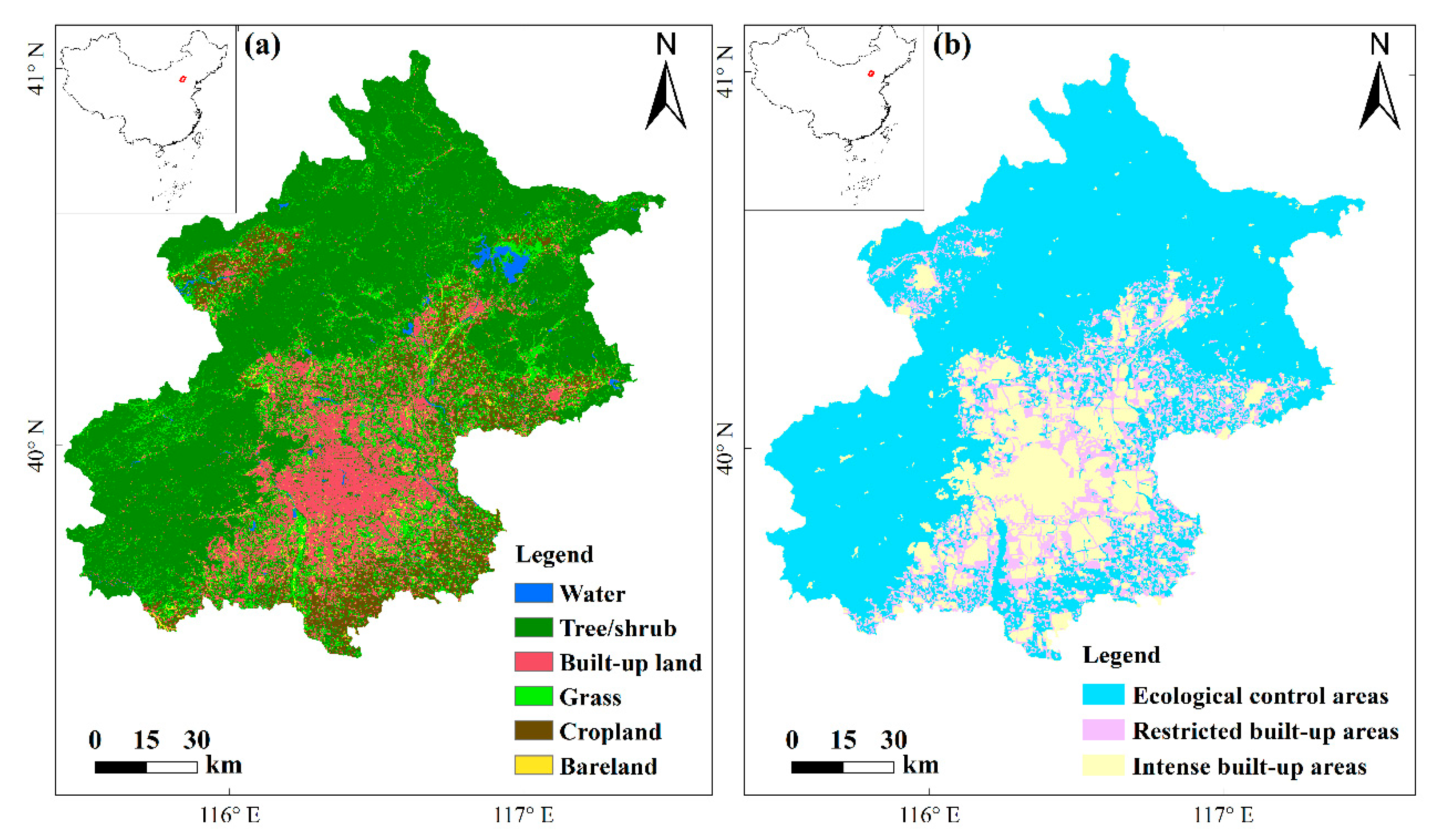
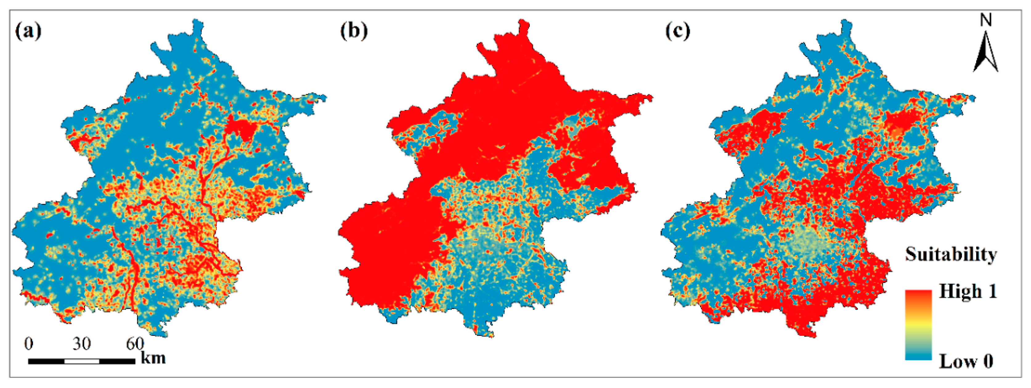
3.1. Habitat Suitability for Focal Species

The final models for the three focal species are shown in

Table 2. Final models for estimating the occupancy (ψ) and detection (p) probability for focal water bird mallard, forest bird grey-headed woodpecker and open-habitat bird Eurasian collared dove in Beijing.

Birds	Models
Water	ψ(water + bareland + grass + dis2water + dis2road)p(date + temperature + precipitation)
Forest	ψ(water + bareland + forest + grass + cropland)p(date + temperature + precipitation)
Open-habitat	ψ(water + bareland + forest + grass/cropland + dis2water)p(date + temperature + precipitation)

Notes: water, bareland, forest, grass, cropland: the percentage of each land cover type within a 600 m-buffer; grass/cropland: grass and cropland; dis2water: distance to the nearest water body. dis2road: distance to the nearest major road.

. Mean detection probability of the mallard (water bird) was the highest ($0.56$), followed by the grey-headed woodpecker (forest bird) ($0.40$), and then the Eurasian collared dove (open habitat bird) ($0.20$).

For mallard, the percentages of water and grass were positively correlated with occupancy probability (

Table 3. The coefficient, standard error and p-value of each variable in the occupancy submodels for the water bird mallard, the forest bird grey-headed woodpecker and the open-habitat bird Eurasian collared dove in Beijing.

Birds	Models	Intercept	Water	Bareland	Forest	Grass	Cropland	Dis2water	Dis2road
Water	Coefficient	11.63	31.39	0.81	-	0.81	-	−0.82	0.25
	SE	5.19	13.56	0.57	-	0.36	-	0.65	0.34
	p-value	0.03	0.02	0.15	-	0.02	-	0.21	0.46
Forest	Coefficient	2.68	0.07	−0.40	3.89	0.05	−0.21	-	-
	SE	0.88	0.29	0.61	1.09	0.32	0.42	-	-
	p-value	0.00	0.81	0.52	0.00	0.89	0.62	-	-
Open habitat	Coefficient	−0.09	0.22	−2.52	−0.36	4.13 *		−1.37	-
	SE	0.59	0.34	1.42	0.48	1.55 *		0.84	-
	p-value	0.88	0.53	0.08	0.45	0.01 *		0.10	-

Notes: Water, bareland, forest, grass, and cropland: the percentage of each land cover type within a 600 m-buffer. Dis2water: distance to the nearest water body; Dis2road: distance to the nearest major road; *: grass and cropland are grouped into one type.

). The most important variable was water and mallard only required relatively low coverage of water (Figure 2a). Suitable habitats for water birds mainly appeared around reservoirs, wetlands, lakes, and rivers (Figure 3a), such as Miyun reservoir in Northeast Beijing, Guanting reservoir and Wild Duck Lake national wetland park in the northwest, as well as wetlands and green spaces along the Chaobai and Wenyu rivers in urban areas (Figure 3a).

For grey-headed woodpecker, the percentage of forest positively influenced occupancy probability and was also the most important variable (Table 3). The occurrence probability of this species sharply increased when the forest cover reached 30% (Figure 2b). Highly suitable areas were concentrated in the northern and southwestern suburban mountain forest and forest in urban green spaces (Figure 3b).

For Eurasian collared dove, the percentage of open habitat (grass and cropland) positively influence occupancy probability (Table 3). The probability of presence increased considerably when the cover of grass and cropland reached 25% (Figure 2c). Suitable habitats for open habitat birds were mainly positioned in Eastern and Southern Beijing in the Fangshan, Daxing, Tongzhou, Shunyi, Pinggu, and Yanqing districts (Figure 3c).

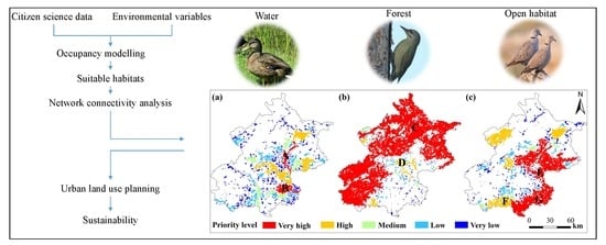
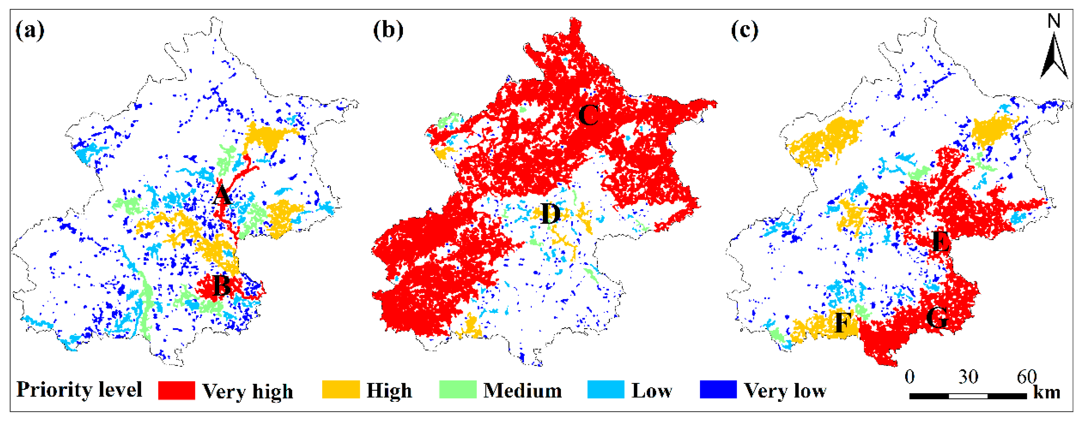
3.2. The Habitat Network Connectivity and Conservation Priority

For the focal water bird species, key habitat patches were mainly distributed in east and central Beijing (the Chaobai river in Shunyi district, the Liangshui and Xiaotaihou rivers in Tongzhou district, the Wenyu and Ba rivers in Chaoyang district, Miyun reservoir in Miyun district, the North Canal and Yunchaojian rivers in Tongzhou district, the Ju and Ru rivers in Pinggu district, the Sha and Wenyu rivers in Changping district, the Qing river in Haidian district and Olympic Park in Chaoayng district) (Figure 4a,

Table A4. Summary of key habitat patches for priority conservation for focal water, forest, and open-habitat bird species in Beijing municipality. Id code refers to the id of the habitat patch. dPC value represents the contribution of the habitat patch to the overall network connectivity. Key patches with over 50% area fall into the restricted built-up areas are marked with an asterisk.

Birds	Id	Patch Name	Area/km2	dPC/%	Situation in Network	Location/(E°, N°)
Water	467 *	Chaobai River in Shunyi district	159.9	34.2	Center of the habitat network	116.741	40.206
	499 *	Liangshui & Xiaotaihou Rivers, wetlands and grass in Tongzhou district	234.1	24.8	Large patch	116.729	39.807
	71 *	Wenyu and Ba Rivers in Chaoyang district	122.0	18.6	Large patch and close to key patches 502, 503	116.605	39.990
	446	Miyun Reservoir	205.8	18.6	Large patch	116.943	40.502
	502 *	North Canal and Yunchaojian Rivers in Tongzhou district	56.3	18.3	Close to large patch 71, 499	116.717	39.908
	464 *	Ju and Ru Rivers in Pinggu district	190.4	15.8	Large patch	117.038	40.129
	504 *	Sha and Wenyu Rivers in Changping district	120.5	14.7	Center of the habitat network	116.348	40.115
	503 *	Qing River and Olympic Park in Chaoyang district	80.4	13.6	Close to key patch 71, 504 and center of the habitat network	116.447	40.045
	501 *	Yueya & Zhongba Rivers and Bojue golf club in Tongzhou district	22.3	12.8	Close to large patch 71	116.714	40.000
Forest	1	Mountains in Yanqing, Huairou and Miyun districts	5289.2	86.1	Large patch	116.661	40.492
	280	Mountains in Fangshan and Shijingshan districts	1821.0	39.3	Large patch	115.934	39.852
	281	Mountains in Mentougou district	1011.7	34.8	Large patch and close to large patch 280, 1	115.773	40.045
	68 *	Forest along the Wenyu River and 6th north ring road in Shunyi district	62.4	1.1	Center of the habitat network	116.496	40.158
	244 *	Forest along the Dashi River in Liulihe town	66.0	0.9	Close to large patch 279	116.015	39.628
	127 *	Forest along the Wenyu River in Chaoyang district	41.7	0.7	Center of the habitat network	116.574	40.018
	34	Forest around Guanting Reservoir and Guishui River in Yanqing district	35.7	0.7	Close to large patch 1	115.854	40.429
	70 *	Forest along the Chaobai River in Shunyi district	45.3	0.6	Center of the habitat network	116.698	40.129
Open habitat	206	Grass/cropland in Daxing and Tongzhou districts	1090.6	53.8	Large patch	116.575	39.693
	78 *	Grass/cropland in Changping, Shunyi and Huairou districts	613.0	39.8	Large patch	116.558	40.263
	324 *	Grass/cropland in Shunyi and Pinggu districts	795.4	36.1	Large patch	116.953	40.189
	307 *	Grass/cropland between Tong zhou, Chaoyang and Shunyi districts	193.7	34.1	Closed to large patches 206, 78,324	116.642	40.014
	310 *	Grass/cropland in Fangshan district	312.5	16.5	Large patch and close to large patch 206	116.012	39.634
	48	Grass/cropland around Miyun Reservoir	222.7	9.4	Large patch	117.025	40.543
	54	Grass/cropland in Yanqing district	455.9	6.9	Large patch	116.005	40.480
	319 *	Grass/cropland around Yangfang town	117.9	6.9	Close to large patch 78 and center of the habitat network	116.168	40.137

, Appendix A). For the focal forest bird species, key patches are found in north and southwest Beijing (Yanqing, Huairou, Miyun, Fangshan, Shijingshan, and Mentougou districts), and central Beijing (the Wenyu river in Shunyi and Chaoyang districts, and the Chaobai river in Shunyi district) (Figure 4b, Table A4, Appendix A). For the focal open-habitat bird species, most of key patches are located in northeast and southeast Beijing (Daxing, Tongzhou, Shunyi, and Yanqing districts) (Figure 4c, Table A4, Appendix A).

Most of the key habitat patches for forest birds (92%) were located in ecological control areas, whereas a small percentage fell into restricted built-up areas (Figure 5). For water and open-area birds, only 37% and 52% of key habitat patches were in ecological control areas (Figure 5). Key habitat patches for water birds in restricted built-up areas, with a total surface area of 321.3 km², were mainly distributed in Northeast Beijing (along the Chaobai, Ru, and Ju rivers), Central Beijing (surroundings of Shahe reservoir and the Wenyu river), and Southwest Beijing (along the Liangshui river in Yizhuang). For forest birds, only 272.9 km² of key habitat patches were located in restricted built-up areas, and mainly located at the foot of the mountains and in the Xiaotangshan modern agricultural park in Changping district. A total of 1036.5 km² of key habitat patches for open-habitat birds occurred in restricted built-up areas, and were mainly distributed in the Daxing, Tongzhou, and Shunyi districts.

4. Discussion

Our study proposes an approach in prioritizing urban green space protection from a focal species habitat network perspective. Using occupancy modelling and citizen science bird observation data, we predicted habitat suitability for three focal water, forest, and open-habitat bird species, presumed to encapsulate the needs of wider species communities. Since different communities show distinct habitat preference, our approach could more accurately quantify habitat patches for targeting communities, compared to simply using green space to delineate the habitat in general. The identified core habitat patches in the habitat networks could guide urban green space management and provide the scientific basis for urban planners to target areas for protection priority in the future development plan. By using focal species of three bird communities as bio-indicators, our study provides evidence-based measures to help maintain urban habitat connectivity and preserve biodiversity.

The quantified habitat requirements, suitable habitat maps and identified core habitat patches for the focal water, forest and open-habitat bird species could guide green space management and urban planning. The focal water bird mallard requires only a relatively low surface area of water, suggesting maintaining or restoring small waterbodies in urban green areas would be an efficient way of maintaining water birds. An alternative explanation would be that most waterbodies in urban areas are relatively small and water birds have adapted to this kind of landscape. On the other hand, frost birds and open-habitat birds need a moderate level of forest and open-habitat cover to survive. This implies that the composition of forest and open-habitat should be taken into account when designing city parks, restoring habitats or setting up conservation plans.

We found that large habitat patches are important in facilitating habitat network connectivity. For example, patch ‘B’, ‘C’, and ‘G’ (Figure 4) are the largest patches in the habitat network of the focal species and are also some of the most important patches in facilitating habitat connectivity. Patch ‘B’ is located in an area composed of rivers (e.g., the Liangshui and Xiaotaihou rivers), wetlands, parks and grassland. Patch ‘C’ is covered by continuous forest and ‘G’ is grass/farmland. Larger patch size contributes to a greater intra-patch and inter-patch connectivity in a habitat network [16,19]. They not only offer a larger area of habitat, but also increase the amount of area-weighted dispersal flux [19] and, hence, should to be protected.

In addition to the size of patches, we found that habitat patches positioned at a critical spatial position in the habitat network are also important for maintaining habitat connectivity. By acting as stepping-stones, patches located in the center of the network and/or near large patches, tend to have a higher contribution to the habitat connectivity. For example, for the representative water bird species, patch ‘A’ (Figure 4a) along the Chaobai River connects surrounding habitat patches. For the representative forest bird species, patch ‘D’ (Figure 4b) along the Wenyu River, acted as a key stepping stone connecting the urban and suburban areas. For the focal open-habitat bird species, patch ‘E’ (Figure 4c) connects the northern and southern key patches. Moreover, patches near large patches (e.g., patch ‘F’ in Figure 4c) not only facilitates species dispersal, but also acts as a barrier against human disturbance [16]. Loss of such key stepping-stone patches might rapidly reduce the overall connectivity and increase the chance of network collapse [75,76]. It is, therefore, important to evaluate sites for conservation priority from a network perspective, instead of only at the site level. Hence, such stepping-stone patches should be prioritized in urban biodiversity conservation [16,37].

We suggest conservation planning takes into account both habitat suitability and habitat network connectivity. As the designation for restricted built-up areas in Beijing is not yet fixed, we suggest that the identified key habitat patches within restricted built-up areas for water and forest birds should be converted into ecological control areas and those for open-habitat communities should be preserved as cropland under future urban planning (Table A4, Appendix A).

We selected focal water, forest and open-habitat birds with distinct habitat preferences. The spatial and functional requirement of these focal species could help define the environmental limits and help protect other species [33]. A rigid selection procedure is critical, given that focal species need to reflect the overall biodiversity of the territory under investigation. Besides the commonly used criteria habitat barycenter [33,48], we also considered the variance of the habitat barycenter. Smaller variance indicates that the species is more selective toward one specific habitat type and uses alternative habitats less. In consequence, by protecting the habitat of selected focal species, other taxonomic groups could also be protected, including those with less observation data available. We underline the usefulness of applying the focal species concept in urban biodiversity conservation.

Our study highlights the combination of occupancy modelling of focal species with network connectivity analysis to identify key habitat patches for conservation prioritization. Species distribution modelling (SDM) has been frequently used to quantify environment-species relationships and generate suitability habitat maps [77] to guide urban wildlife protection and biodiversity conservation (e.g., [32,78]). The habitat network connectivity has hardly been investigated after suitable habitat has been delineated using SDM (except for [22,48,79]). In real world conservation, not all suitable habitat can be protected, especially under ongoing urbanization. The quantification of the core habitat patches from a habitat network connectivity perspective offers an efficient way to target the most important areas for protection priority. In addition, we built the occupancy model based on 10-year bird observation data and the 2015 land cover map, mainly due to the limited number of bird records. We recommend promoting the collection of citizen science data, as more observations and observation sites would improve the prediction of suitable habitat patches. Nevertheless, our approach of coupling focal specie occupancy modelling with network analysis to guide conservation efforts could be applied to other cities, where fine resolution land cover map and bird observation data are available.

5. Conclusions

Since habitat fragmentation causes biodiversity loss, it is necessary to protect urban biodiversity based on habitat suitability and the functional connectivity of the habitat network. We select three focal species presuming their habitat requirements encapsulate many other species and underline their usefulness in urban biodiversity conservation. Based on the habitat requirement, small waterbodies and intermediate forest and open-habitat cover facilitate preserving water, forest, and open-habitat bird communities, respectively. In light of the network analysis, key habitat patches with a high conservation priority are generally characterized by having a large surface area and/or being located at critical positions in the habitat network (i.e., at central positions in the habitat network and/or near large patches). We suggest that urban planners preserve such key patches in restricted built-up areas (Table A4, Appendix A) in future urban development plans. We consider that the evaluation of individual habitat patches in terms of conservation priority, based on the contribution of these patches to habitat network connectivity, is an effective method to optimize decision-making in future urban conservation planning. Our findings provide guidelines for the conservation of local biodiversity and sustainable urban development.

References

1. United Nations: Department of Economic and Social Affairs. World Urbanization Prospects: The 2018 Revision; United Nations: Department of Economic and Social Affairs: New York, NY, USA, 2018. [Google Scholar]
2. China Statistical Press. China Statistical Yearbook in 2018; China Statistical Press: Beijing, China, 2018. (In Chinese) [Google Scholar]
3. Grimm, N.B.; Faeth, S.H.; Golubiewski, N.E.; Redman, C.L.; Wu, J.; Bai, X.; Briggs, J.M. Global Change and the Ecology of Cities. Science 2008, 319, 756–760. [Google Scholar] [CrossRef]
4. Xun, B.; Yu, D.; Liu, Y.; Hao, R.; Sun, Y. Quantifying isolation effect of urban growth on key ecological areas. Ecol. Eng. 2014, 69, 46–54. [Google Scholar] [CrossRef]
5. Ortega-Álvarez, R.; MacGregor-Fors, I. Living in the big city: Effects of urban land-use on bird community structure, diversity, and composition. Landsc. Urban Plan. 2009, 90, 189–195. [Google Scholar] [CrossRef]
6. Canedoli, C.; Orioli, V.; Padoa-Schioppa, E.; Bani, L.; Dondina, O. Temporal Variation of Ecological Factors Affecting Bird Species Richness in Urban and Peri-Urban Forests in a Changing Environment: A Case Study from Milan (Northern Italy). Forests 2017, 8, 507. [Google Scholar] [CrossRef]
7. Alberti, M. The Effects of Urban Patterns on Ecosystem Function. Int. Reg. Sci. Rev. 2005, 28, 168–192. [Google Scholar] [CrossRef]
8. Opdam, P.; Steingröver, E.; Rooij, S.V. Ecological networks: A spatial concept for multi-actor planning of sustainable landscapes. Landsc. Urban Plan. 2006, 75, 322–332. [Google Scholar] [CrossRef]
9. Defries, R.S.; Foley, J.A.; Asner, G.P. Land-use choices: Balancing human needs and ecosystem function. Front. Ecol. Environ. 2004, 2, 249–257. [Google Scholar] [CrossRef]
10. Wilson, E.; MacArthur, R. The Theory of Island Biogeography; Princeton University Press: Princeton, NJ, USA, 2001. [Google Scholar]
11. Diamond, J.M. The island dilemma: Lessons of modern biogeographic studies for the design of natural reserves. Biol. Conserv. 1975, 7, 129–146. [Google Scholar] [CrossRef]
12. Cody, M.L.; Diamond, J.M. Ecology and Evolution of Communities. Nature 1976, 260, 204. [Google Scholar] [CrossRef]
13. Margules, C.R.; Pressey, R.L. Systematic conservation planning. Nature 2000, 405, 243–253. [Google Scholar] [CrossRef]
14. Taylor, P.D.; Fahrig, L.; Henein, K.; Merriam, G. Connectivity is a vital element of landscape structure. Oikos 1993, 68, 571–573. [Google Scholar] [CrossRef]
15. Saura, S.; Pascual-Hortal, L. A new habitat availability index to integrate connectivity in landscape conservation planning: Comparison with existing indices and application to a case study. Landsc. Urban Plan. 2007, 83, 91–103. [Google Scholar] [CrossRef]
16. Xun, B.; Yu, D.; Wang, X. Prioritizing habitat conservation outside protected areas in rapidly urbanizing landscapes: A patch network approach. Landsc. Urban Plan. 2017, 157, 532–541. [Google Scholar] [CrossRef]
17. Uezu, A.; Metzger, J.P.; Vielliard, J.M.E. Effects of structural and functional connectivity and patch size on the abundance of seven Atlantic Forest bird species. Biol. Conserv. 2005, 123, 507–519. [Google Scholar] [CrossRef]
18. Hüse, B.; Szabó, S.; Deák, B.; Tóthmérész, B. Mapping an ecological network of green habitat patches and their role in maintaining urban biodiversity in and around Debrecen city (Eastern Hungary). Land Use Policy 2016, 57, 574–581. [Google Scholar] [CrossRef]
19. Saura, S.; Rubio, L. A common currency for the different ways in which patches and links can contribute to habitat availability and connectivity in the landscape. Ecography 2010, 33, 523–537. [Google Scholar] [CrossRef]
20. Pascual-Hortal, L.; Saura, S. Impact of spatial scale on the identification of critical habitat patches for the maintenance of landscape connectivity. Landsc. Urban Plan. 2007, 83, 176–186. [Google Scholar] [CrossRef]
21. Kang, W.; Minor, E.S.; Park, C.R.; Lee, D. Effects of habitat structure, human disturbance, and habitat connectivity on urban forest bird communities. Urban Ecosyst. 2015, 18, 857–870. [Google Scholar] [CrossRef]
22. Fajardo, J.; Lessmann, J.; Bonaccorso, E.; Devenish, C.; Muñoz, J. Combined use of systematic conservation planning, species distribution modelling, and connectivity analysis reveals severe conservation gaps in a megadiverse country (Peru). PLoS ONE 2014, 9, e114367. [Google Scholar] [CrossRef]
23. Gao, Y.; Ma, L.; Liu, J.; Zhuang, Z.; Huang, Q.; Li, M. Constructing Ecological Networks Based on Habitat Quality Assessment: A Case Study of Changzhou, China. Sci. Rep. 2017, 7, 46073. [Google Scholar] [CrossRef]
24. Dondina, O.; Orioli, V.; Colli, L.; Luppi, M.; Bani, L. Ecological network design from occurrence data by simulating species perception of the landscape. Landsc. Ecol. 2018, 33, 275–287. [Google Scholar] [CrossRef]
25. Dondina, O.; Orioli, V.; Chiatante, G.; Alberto, M.; Bani, L. Species Specialization Limits Movement Ability and Shapes Ecological Networks: The Case Study of two Forest Mammals. Curr. Zool. 2018. [Google Scholar] [CrossRef]
26. Dondina, O.; Saura, S.; Bani, L.; Mateo-Sánchez, M.C. Enhancing connectivity in agroecosystems: Focus on the best existing corridors or on new pathways? Landsc. Ecol. 2018, 33, 1741–1756. [Google Scholar] [CrossRef]
27. Li, F.; Wang, R.; Paulussen, J.; Liu, X. Comprehensive concept planning of urban greening based on ecological principles: A case study in Beijing, China. Landsc. Urban Plan. 2005, 72, 325–336. [Google Scholar] [CrossRef]
28. Kong, F.; Yin, H.; Nakagoshi, N.; Zong, Y. Urban green space network development for biodiversity conservation: Identification based on graph theory and gravity modeling. Landsc. Urban Plan. 2010, 95, 16–27. [Google Scholar] [CrossRef]
29. Dickinson, J.L.; Zuckerberg, B.; Bonter, D.N. Citizen Science as an Ecol. Res. Tool: Challenges and Benefits. Annu. Rev. Ecol. Syst. 2010, 41, 149–172. [Google Scholar] [CrossRef]
30. Strien, A.J.; Swaay, C.A.M.; Termaat, T.; Devictor, V. Opportunistic citizen science data of animal species produce reliable estimates of distribution trends if analysed with occupancy models. J. Appl. Ecol. 2013, 50, 1450–1458. [Google Scholar] [CrossRef]
31. Mackenzie, D.I. Occupancy Estimation and Modeling; Elsevier: Amsterdam, The Netherlands, 2006. [Google Scholar]
32. De Wan, A.A.; Sullivan, P.J.; Lembo, A.J.; Smith, C.R.; Maerz, J.C.; Lassoie, J.P.; Richmond, M.E. Using occupancy models of forest breeding birds to prioritize conservation planning. Biol. Conserv. 2009, 142, 982–991. [Google Scholar] [CrossRef]
33. Padoa-Schioppa, E.; Baietto, M.; Massa, R.; Bottoni, L. Bird communities as bioindicators: The focal species concept in agricultural landscapes. Ecol. Indic. 2006, 6, 83–93. [Google Scholar] [CrossRef]
34. Ogden, J.C.; Baldwin, J.D.; Bass, O.L.; Browder, J.A.; Cook, M.I.; Frederick, P.C.; Frezza, P.E.; Galvez, R.A.; Hodgson, A.B.; Meyer, K.D.; et al. Waterbirds as indicators of ecosystem health in the coastal marine habitats of southern Florida: 1. Selection and justification for a suite of indicator species. Ecol. Indic. 2014, 44, 148–163. [Google Scholar] [CrossRef]
35. Rahman, F.; Ismail, A. Waterbirds: An important bio-indicators of ecosystem. Pertanika J. Schol. Res. Rev. 2018, 4, 81–90. [Google Scholar]
36. Li, X.; Gong, P.; Liang, L. A 30-year (1984–2013) record of annual urban dynamics of Beijing City derived from Landsat data. Remote Sens. Environ. 2015, 166, 78–90. [Google Scholar] [CrossRef]
37. Strohbach, M.W.; Lerman, S.B.; Warren, P.S. Are small greening areas enhancing bird diversity? Insights from community-driven greening projects in Boston. Landsc. Urban Plan. 2013, 114, 69–79. [Google Scholar] [CrossRef]
38. Silva de Araújo, M.L.V.; Bernard, E. Green remnants are hotspots for bat activity in a large Brazilian urban area. Urban Ecosyst. 2016, 19, 287–296. [Google Scholar] [CrossRef]
39. Fuyuki, A.; Yamaura, Y.; Nakajima, Y.; Ishiyama, N.; Akasaka, T.; Nakamura, F. Pond area and distance from continuous forests affect amphibian egg distributions in urban green spaces: A case study in Sapporo, Japan. Urban For. Urban Green. 2014, 13, 397–402. [Google Scholar] [CrossRef]
40. Threlfall, C.G.; Walker, K.; Williams, N.S.G.; Hahs, A.K.; Mata, L.; Stork, N.; Livesley, S.J. The conservation value of urban green space habitats for Australian native bee communities. Biol. Conserv. 2015, 187, 240–248. [Google Scholar] [CrossRef]
41. Luppi, M.; Dondina, O.; Orioli, V.; Bani, L. Local and landscape drivers of butterfly richness and abundance in a human-dominated area. Agric. Ecosyst. Environ. 2018, 254, 138–148. [Google Scholar] [CrossRef]
42. Hu, W.; Wang, S.; Li, D. Biological conservation security patterns plan in Beijing based on the focal species approach (in Chinese). Acta Ecol. Sin. 2010, 30, 4266–4276. [Google Scholar]
43. China Bird Report Center. Available online: http://www.birdreport.cn (accessed on 21 December 2017).
44. Li, X.; Liang, L.; Gong, P.; Liu, Y.; Liang, F. Bird watching in China reveals bird distribution changes. Chin. Sci. Bull. 2013, 58, 649–656. [Google Scholar] [CrossRef]
45. Hamish, W.; Jonathan, B.; Jennifer, S.; Carolina, D.L.R.; Rivadeneira, M.; Walter, J. EltonTraits 1.0: Species-level foraging attributes of the world’s birds and mammals. Ecology 2014, 95, 2027. [Google Scholar] [CrossRef]
46. Brazil, M. Birds of East Asia; Christopher Helm: London, UK, 2009. [Google Scholar]
47. Lambeck, R.J. Focal Species: A multi-species umbrella for nature conservation. Conserv. Biol. 1997, 11, 849–856. [Google Scholar] [CrossRef]
48. Bani, L.; Baietto, M.; Bottoni, L.; Massa, R. The use of focal species in designing a habitat network for a lowland area of Lombardy, Italy. Conserv. Biol. 2002, 16, 826–831. [Google Scholar] [CrossRef]
49. Hijmans, R.J. Raster: Geographic Data Analysis and Modeling. R Package Version 2.8-19. Available online: https://cran.r-project.org/web/packages/raster/index.html (accessed on 25 March 2017).
50. R Core Team. R: A Language and Environment for Statistical Computing; R Foundation for Statistical Computing: Vienna, Austria, 2015. [Google Scholar]
51. Huang, C.; Yang, J.; Lu, H.; Huang, H.; Yu, L. Green Spaces as an Indicator of Urban Health: Evaluating Its Changes in 28 Mega-Cities. Remote Sens. 2017, 9, 1266. [Google Scholar] [CrossRef]
52. Advanced Spaceborne Thermal Emission and Reflection Radiometer Global Digital Elevation Model. Available online: http://reverb.echo.nasa.gov/reverb/ (accessed on 27 May 2018).
53. Vector Data of Major Roads. Available online: http://www.bjdata.gov.cn/zyml/ajg/sgtj/5173.htm (accessed on 15 August 2018).
54. Operational Linescan System (OLS) by the U.S. Air Force Defense Meteorological Satellite Program (DMSP)/Version 4 DMSP-OLS Nighttime Lights Time Series. Available online: https://ngdc.noaa.gov/eog/dmsp/downloadV4composites.html (accessed on 18 August 2018).
55. Land Surface Temperature/Emissivity Monthly L3 Global 0.05Deg CMG. Available online: https://e4ftl01.cr.usgs.gov/MOLT/ (accessed on 5 August 2018).
56. European Centre for Medium-Range Weather Forecasts (ECMWF) ERA-Interim, Monthly means of Daily Forecast Accumulations. Available online: http://apps.ecmwf.int/datasets/data/interim-mdfa/levtype=sfc/ (accessed on 6 August 2018).
57. Huang, Y.; Zhao, Y.; Li, S.; von Gadow, K. The Effects of habitat area, vegetation structure and insect richness on breeding bird populations in Beijing urban parks. Urban For. Urban Green. 2015, 14, 1027–1039. [Google Scholar] [CrossRef]
58. McGarigal, K.; Cushman, S.A.; Ene, E. FRAGSTATS v4: Spatial Pattern Analysis Program for Categorical Maps; Computer software program produced by the authors at the University of Massachusetts: Amherst, MA, USA, 2012; Available online: http://www.umass.edu/landeco/research/fragstats/fragstats.html (accessed on 13 April 2017).
59. Li, X.; Si, Y.; Ji, L.; Gong, P. Dynamic response of East Asian Greater White-fronted Geese to changes of environment during migration: Use of multi-temporal species distribution model. Ecol. Model. 2017, 360, 70–79. [Google Scholar] [CrossRef]
60. Rosin, Z.M.; Piotr, S.; Paweł, S.; Marcin, T.; Andrzej, L.; Piotr, T. Constant and seasonal drivers of bird communities in a wind farm: Implications for conservation. PeerJ 2016, 4, e2105. [Google Scholar] [CrossRef]
61. Summers, P.D.; Cunnington, G.M.; Fahrig, L. Are the negative effects of roads on breeding birds caused by traffic noise? J. Appl. Ecol. 2011, 48, 1527–1534. [Google Scholar] [CrossRef]
62. Orłowski, G. Roadside hedgerows and trees as factors increasing road mortality of birds: Implications for management of roadside vegetation in rural landscapes. Landsc. Urban Plan. 2008, 86, 153–161. [Google Scholar] [CrossRef]
63. Ghosh, T.; Anderson, S.J.; Elvidge, C.D.; Sutton, P.C. Using nighttime satellite imagery as a proxy measure of human well-being. Sustainability 2013, 5, 4988–5019. [Google Scholar] [CrossRef]
64. Strittholt, J.R.; Dellasala, D.A. Importance of Roadless Areas in Biodiversity Conservation in Forested Ecosystems: Case Study of the Klamath-Siskiyou Ecoregion of the United States. Conserv. Biol. 2001, 15, 1742–1754. [Google Scholar] [CrossRef]
65. Dormann, C.F.; Elith, J.; Bacher, S.; Buchmann, C.; Carl, G.; Carré, G.; Marquéz, J.R.G.; Gruber, B.; Lafourcade, B.; Leitão, P.J.; et al. Collinearity: A review of methods to deal with it and a simulation study evaluating their performance. Ecography 2013, 36, 27–46. [Google Scholar] [CrossRef]
66. ESRI. ArcGIS Desktop: Release 10.3.1; Environmental Systems Research Institute: Redlands, CA, USA, 2015. [Google Scholar]
67. Fiske, I.J.; Chandler, R.B. Unmarked: An R package for fitting hierarchical models of wildlife occurrence and abundance. J. Stat. Softw. 2011, 43, 1–23. [Google Scholar] [CrossRef]
68. Bartoń, K. MuMIn: Multi-Model Inference, R Package Version 1.42.1; Available online: https://cran.rstudio.com/web/packages/MuMIn/ (accessed on 23 November 2017).
69. Burnham, K.P.; Anderson, D.R. Model Selection and Multimodel Inference: A Practical Information-Theoretic Approach, 2nd ed.; Springer: New York, NY, USA, 2002. [Google Scholar]
70. MacKenzie, D.I.; Bailey, L.L. Assessing the fit of site-occupancy models. J. Agric. Biol. Environ. Stat. 2004, 9, 300–318. [Google Scholar] [CrossRef]
71. Symonds, M.R.E.; Moussalli, A. A brief guide to model selection, multimodel inference and model averaging in behavioural ecology using Akaike’s information criterion. Behav. Ecol. Sociobiol. 2011, 65, 13–21. [Google Scholar] [CrossRef]
72. Liu, C.; Berry, P.M.; Dawson, T.P.; Richard, G. Pearson Selecting thresholds of occurrence in the prediction of species distributions. Ecography 2005, 28, 385–393. [Google Scholar] [CrossRef]
73. Saura, S.; Torné, J. Conefor Sensinode 2.2: A software package for quantifying the importance of habitat patches for landscape connectivity. Environ. Model. Softw. 2009, 24, 135–139. [Google Scholar] [CrossRef]
74. Jenks, G.F. The Data Model Concept in Statistical Mapping. Int. Yearb. Cartogr. 1967, 7, 186–190. [Google Scholar]
75. Shimazaki, H.; Tamura, M.; Darman, Y.; Andronov, V.; Parilov, M.P.; Nagendran, M.; Higuchi, H. Network analysis of potential migration routes for Oriental White Storks (Ciconia boyciana). Ecol. Res. 2004, 19, 683–698. [Google Scholar] [CrossRef]
76. Saura, S.; Bodin, Ö.; Fortin, M.-J. Editor’s choice: Stepping stones are crucial for species’ long-distance dispersal and range expansion through habitat networks. J. Appl. Ecol. 2014, 51, 171–182. [Google Scholar] [CrossRef]
77. Li, X.; Wang, Y. Applying various algorithms for species distribution modelling. Integr. Zool. 2013, 8, 124–135. [Google Scholar] [CrossRef]
78. Tiwary, N.K.; Urfi, A.J. Spatial variations of bird occupancy in Delhi: The significance of woodland habitat patches in urban centres. Urban For. Urban Green. 2016, 20, 338–347. [Google Scholar] [CrossRef]
79. Merken, R.; Deboelpaep, E.; Teunen, J.; Saura, S.; Koedam, N. Wetland Suitability and Connectivity for Trans-Saharan Migratory Waterbirds. PLoS ONE 2015, 10, e0135445. [Google Scholar] [CrossRef]
Figure 1. Map of the study area. (a) The 2015 land cover map of Beijing municipality, and (b) the layout of the ecological control areas, restricted built-up areas and intense built-up areas in the Beijing Urban Master Plan (2016–2035).
Sustainability 11 02042 g001
Figure 2. Response curves illustrating the relationship between the environmental factors (only the most important variables were presented) and the occupancy probability of the water bird mallard (a), the forest bird grey-headed woodpecker (b), and the open-habitat bird Eurasian collared dove (c). Open habitat refers to grassland and cropland. The grey areas indicate the 95% confidence interval.
Sustainability 11 02042 g002
Figure 3. The habitat suitability map for water bird mallard (a), forest bird grey-headed woodpecker (b), and open-habitat bird Eurasian collared dove (c) in Beijing municipality.
Sustainability 11 02042 g003
Figure 4. Rank of habitat patches with conservation priority based on their contribution to the habitat network connectivity for the water bird mallard (a), the forest bird grey-headed woodpecker (b), and the open-habitat bird Eurasian collared dove (c) in Beijing municipality. White area represents unsuitable habitat. A: Chaobai river in Shunyi district; B: Liangshui and Xiaotaihou rivers in Tongzhou district; C: forest in Yanqing, Huairou and Miyun districts; D: Wenyu river in Shunyi district; E: grass and cropland in Tong zhou, Chaoyang and Shunyi districts; F: grass and cropland in Fangshan district; G: grass and cropland in Daxing and Tongzhou districts.
Sustainability 11 02042 g004
Figure 5. The distribution of key habitat patches with high conservation priority (high or very high levels) inside (protected) and outside (non-protected) of the current ecological control areas for focal water, forest, and open-habitat bird species in Beijing municipality.
Sustainability 11 02042 g005