A Hybrid GA with Variable Quay Crane Assignment for Solving Berth Allocation Problem and Quay Crane Assignment Problem Simultaneously

Abstract

Container terminals help countries to sustain their economic development. Improving the operational efficiency in a container terminal is important. In past research, genetic algorithms (GAs) have been widely used to cope with seaside operational problems, including the berth allocation problem (BAP) and quay crane assignment problem (QCAP) individually or simultaneously. However, most GA approaches in past studies were dedicated to generate time-invariant QC assignment that does not adjust QCs assigned to a ship. This may underutilize available QC capacity. In this research, three hybrid GAs (HGAs) have been proposed to deal with the dynamic and discrete BAP (DDBAP) and the dynamic QCAP (DQCAP) simultaneously. The three HGAs supports variable QC assignment in which QCs assigned to a ship can be further adjusted. The three HGAs employ the same crossover operator but a different mutation operator and a two-stage procedure is used. In the first stage, these HGAs can generate a BAP solution and a QCAP solution that is time-invariant. The time-invariant QC assignment solution is then further transformed into a variable one in the second stage. Experiments have been conducted to investigate the effects of the three HGA and the results showed that these HGAs outperformed traditional GAs in terms of fitness value. In particular, the HGA3 with Thoros mutation operator had the best performance.

1. Introduction

Maritime transport is essential to a country as it plays a major role for international trading that can sustain economic development. It is noted that about 60% of the maritime transports employed containers, with a growth rate of 6.4% each year [1]. This shows that container terminals are important infrastructure sustaining global economic development. How to improve the operational efficiency in a container terminal is definitely an important issue.

Being an integrated part of the global transportation network, container terminals help deliver various products to consumers. Due to its importance, improving the operational efficiency of a container terminal is necessary. In a container terminal there are three operational areas: seaside, yard and landside [2]. Among them, the operations in the seaside area are considered critical as they depend on the berth and quay crane, which are two rare resources that can affect the performance of a container terminal considerably. This has motivated us to focus on improving the operations in the seaside area.

There are three famous seaside operational problems in a container terminal. They are the berth allocation problem (BAP), quay cranes assignment problem (QCAP), and quay cranes scheduling problem (QCSP). In this research, both BAP and QCAP are simultaneously focused. The BAP is a problem of allocating berths to ships while the QCAP is a problem of assigning QCs to ships. In the past, various approaches have been proposed to cope with the BAP and QCAP simultaneously or individually, and these approaches can be exact or approximate. The exact approaches aim to solve problems to optimality. This kind of approaches, however, is fond likely to become computationally intractable when dealing with a problem of practical size, due to non-deterministic polynomial (NP)-hard [3]. Consequently, approximate approaches have been popular, especially heuristics/metaheuristics have become increasingly used. One of the metaheuristics, the genetic algorithm (GA) approaches have been playing the major role in dealing with seaside operational problems [3].

Before dealing with a BAP, understanding its types is necessary. It is found that a BAP usually features two main factors: the arrival time of ship and the configuration of a quay used to accommodate calling ships. When taking the factor of arrival time of ship into consideration, a BAP is featured as a static or dynamic one. In the static BAP, this only considers arrived ships while in the dynamic BAP (DBAP) it also takes incoming ships into account. Due to the fact that ships continue to come during BAP planning, the DBAP is thus focused in this research. When taking the factor of quay configuration, a BAP can be featured as a discrete or continuous one. The discrete BAP separates a quay into fixed sections to accommodate calling ships while the continuous BAP treats the quay entirely as a continuous line so as to accommodate ships as much as possible at one time. Both types of quay configuration exist in the world. However, this research only focuses on the dynamic and discrete BAP (DDBAP). Accordingly, the version of dynamic QCAP (DQCAP) is focused in this research to align with the dynamic BAP that also considers incoming ships [2].

The BAP and QCAP were often solved separately [4,5,6,7]. One disadvantage of a separate study is that it tends to result in poor overall system performance due to the lack of considering interrelationships among different levels of seaside operational problems simultaneously [8]. Another disadvantage found for a BAP-only study is that it often needs to assume fixed handling times for ships because these handling times cannot be estimated based on their assigned number of QCs [6]. For improvement, it has been suggested to solve the seaside operational problems in an integrated way [8]. With respect to the approaches for dealing with the seaside operational problems, it is found that GAs have been widely used [4]. Relevant studies include [9,10,11,12,13]. However, when dealing with the QCAP, these GA approaches have been mostly used to yield time-invariant QC assignment based on a planning framework with fixed time intervals. One disadvantage found for the time-invariant QC assignment is that it cannot best utilize available QCs that have been released by leaving ships. As a result, overall QC capacity will not be best utilized. The disadvantage found for the planning framework that employs fixed time intervals is that it may waste some QC capacity as a QC has to be assigned to a fixed time interval fully. For example, a QC is assigned to a 1 h-interval planning framework to work for a ship but in fact that ship only requires a QC capability of 45 min. As a result this, planning will lead to 15 min of spare time for this QC. For improvement, in this research the variable QC assignment and the variable-interval planning framework are introduced. The variable QC assignment allows QC adjustment to a ship to best utilize released QCs while the variable-interval planning framework only allocates necessary QC capacity to a ship.

To overcome the disadvantages mentioned above, in this research three hybrid GAs (HGAs) have been developed to cope with the DDBAP together with the DQCAP. Based on a variable-time planning framework, each of the HGAs hybrids a specific GA with an event-based heuristic to generate variable QC assignment. These HGAs have a same crossover operator (Two-Point Crossover, TPX) but a different mutation operator. Specifically, HGA1 uses Swap mutation; HGA2 adopts Thoras mutation; HGA3 employs Thoros mutation. A variable QC assignment is derived through a two-stage procedure. Our experiments showed the HGAs with variable QC assignment outperformed a traditional GA with time-invariant QC assignment. Among the three HGAs, the HGA3 with Thoros mutation has the best performance in terms of fitness value (FV).

The other part of this paper is organized as follows. Section 2 provides a literature review. Section 3 mainly focuses on defining and formulating the simultaneous DDBAP and DQCAP. Section 4 formulates the simultaneous DDBAP and DQCAP. Section 4 introduces GA models and the HGAs developed in this research. Section 5 reports experimental methods and discusses experimental results. Finally, Section 6 gives a conclusion and highlights directions of future research.

2. Literature Review

2.1. Berth Allocation Problem (BAP)-Only Studies

BAP-only studies are reviewed as follows. Brown et al. [14] is one early study focusing solving the static BAP. In that study, the authors used an integer programming model (IPM) to find optimal ship-to-berth assignments. However, that study was based on a naval port that has different situations and conditions from a commercial port. Focusing on the commercial ports in Japan, Imai et al. [15] moved to deal with the DBAP study, taking into ship priority into consideration. Finally, the authors concluded the First Come First Served (FCFS) rule is unsuitable to find an optimal ship-to-berth assignment in terms of throughput. It is found that to be more practical recent studies have increasingly focused on the dynamic BAP (DBAP) due to the fact that ships continue to call when BAP planning. For example, Imai et al. [16] dealt with the DBAP by using a subgradient approach. In Reference [17], the authors further proposed a GA approach to solve the same problem as they found the solution procedure of the subgradient approach was still too complicated. In Reference [18], the authors proposed a variable neighborhood search (VNS) to solve the DBAP. The objective of this research was to find the solution with minimum cost that includes sub-costs of waiting, handling and earliness or tardiness of completion. Golias et al. [19] treated the discrete and dynamic berth allocation problem as a multi-objective combinatorial optimization problem in which vessel service is differentiated based on priority agreements. Then, a GA-based heuristic was developed to solve the problem. The results showed that the heuristic had the capability to solve large and real-life instances. Saharidis et al. [20] proposed a hierarchical optimization framework to deal with the discrete and dynamic BAP in a container teminal. A two-level hierarchy was employed. It differentiates between two conflicting objectives that terminal operators face when assigning ships to berths. Based on the k-th best algorithm, an interactive algorithm was developed for the case where multi-objective functions were considered in the upper level. Computational examples in that study showed that the proposed algorithm was capable of finding the optimal/near optimal solution. Xu et al. [21] proposed a heuristic to solve the DBAP, taking factors such as water depth and tidal effects into consideration. They found that a better decision can be achieved if these factors have been taken into account. Lalla-Ruiz et al. [22] proposed a set-partitioning-based model for BAP under time-dependent limitations. Ursavas et al. [23] proposed optimal policies for the BAP under a stochastic nature. Dulebenets [24] used a novel memetic algorithm with a deterministic parameter control for efficient berth scheduling at marine container terminals. Umang et al. [25] proposed real-time management of berth allocation with stochastic arrival and handling times. Zhen et al. [26] examined daily berth planning in a tidal port with channel flow control. Dulebenets [27] applied evolutionary computation for berth scheduling at marine container terminals. Dulebenets et al. [28] proposed a self-adaptive evolutionary algorithm for the berth scheduling problem.

2.2. Simultaneous BAP and Quay Crane Assignment Problem (QCAP) Studies

The DBAP and QCAP have been increasingly solved at the same time. In [9] the authors first formulated the DBAP and the QCAP as an integer programming model (IPM). The objective was to minimize total service time. Then, the two problems were solved by using a GA-based heuristic. A crane transfer scheduling algorithm, based on the maximum flow problem, was used to find the QCAP solution. The GA-based heuristic was found to be capable of finding an approximate solution for the two problems. However, the QCAP solution is time-invariant. Zhou et al. [10] also employed a GA approach to cope with the DBAP and QCAP simultaneously. They also formulated the two problems as a 0–1 non-linear programming model. In that study, the arrival times and handling times of calling ships were treated as stochastic variables. However, that GA approach can only yield time-invariant QC assignment. Liang et al. [5] proposed a HGA to cope with the DBAP and QCAP at the same time. An IPM was formulated in that study with the aim to find the minimized cost solution that considers sub-costs of waiting, handling and delay. That HGA was able to find an approximate solution for both problems. However, the QCAP solution is still a time-invariant one. In addition, it did not consider the costs of QC setups and movements. In [13] the authors further improved the HGA by considering the factors including QC movements and ship priority. However, that HGA still can only perform time-invariant QC assignment. Han et al. [12] also employed a GA to cope with the DBAP and QCAP simultaneously. Similar to Zhou et al. [10], the authors treated the arrival times and handling times of calling ships as stochastic variables and solve the two problems by using the GA approach. The objective of the GA was aimed to find the solution minimizing the expected value plus standard deviation of total service time and weighted tardiness time for all calling ships. The solutions obtained were further evaluated by the simulation approach. Giallombardo et al. [29] dealt with the BAP (TBAP) and QCAP at the tactical level. A two-level approach was employed. At the upper level, a Tabu search method was used to allocate berths; at the lower level, mathematical programming was used to update QCs profile. The two-level approach was able to support variable QC assignment. However, it did not use GA. Li et al. [30] solved the berth and quay crane coordinated scheduling using a multi-objective chaos cloud particle swarm optimization algorithm. Xiang et al. [31] used a reactive strategy for discrete berth allocation and quay crane assignment problems under uncertainty.

The above literature showed that the simultaneous DBAP and DQCAP have been mostly solved by GA approaches. However, these GA-based approaches can only support time-invariant QC assignment.

3. The Definition and Formulation of the Simultaneous Dynamic and Discrete BAP (DDBAP) and Dynamic QCAP (DQCAP)

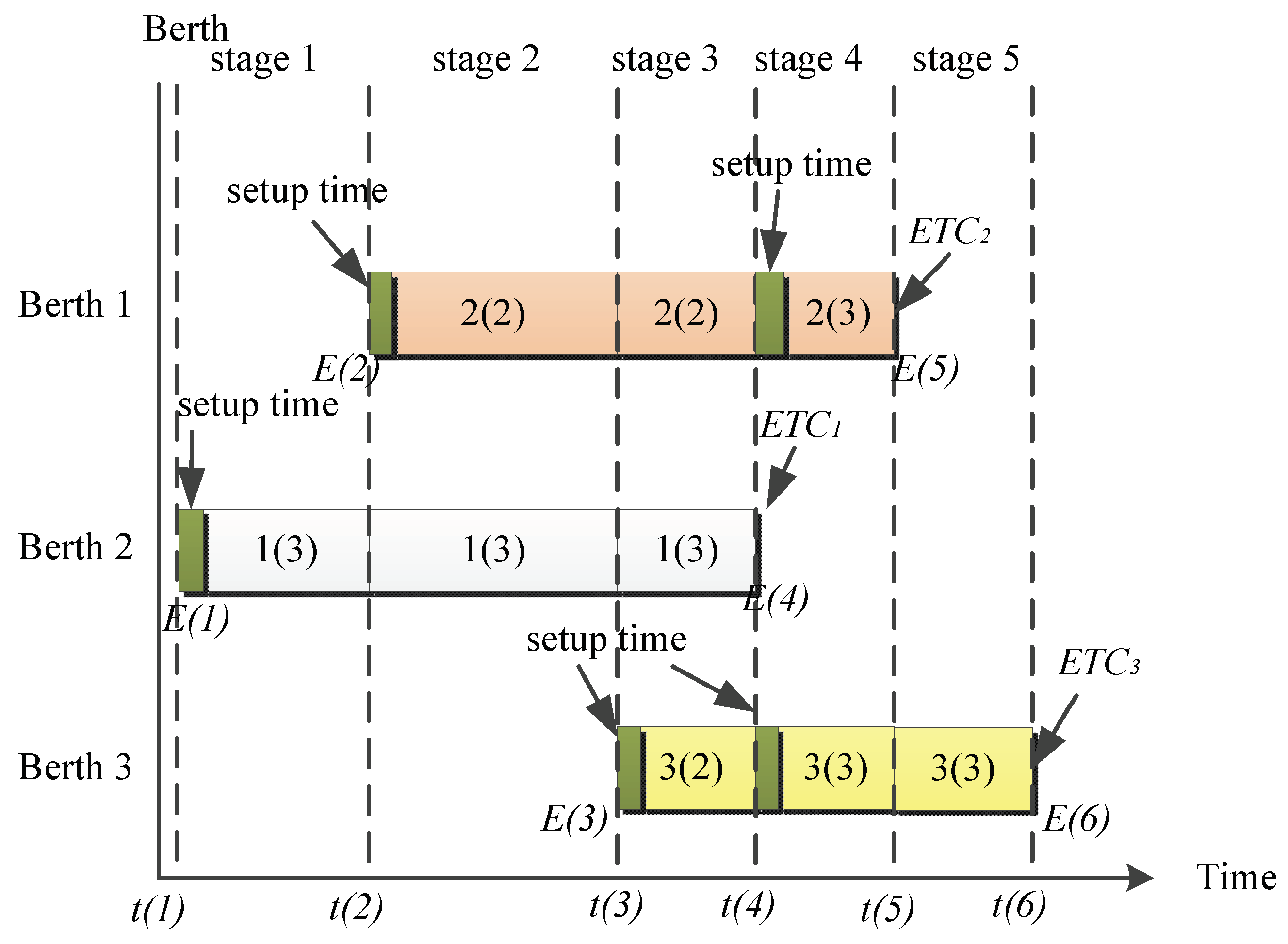
3.1. Berth Plans with Different QC Assignment

A berth plan has been usually used to represent a solution to the simultaneous DDBAP and DQCAP. Figure 1a illustrates a berth plan with time-invariant QC assignment in which each rectangle represents a ship. For example, the rectangle with the denotation “1(3)” indicates that ship 1 is assigned with 3 QCs. With the time-invariant QC assignment, each ship has one time of QC setups and movements for assigned QCs with these QCs not to be further changed during the whole service.

Figure 1b shows a berth plan with variable QC assignment, in which a ship has more than one times of QC setups and movements due to QC reassignments. For instance, ship 2 has two times of QC setups and movements, one at t(2) and another at t(3). Obviously, the variable QC assignment is more flexible at the costs of more QC setups and movements. But the gain and cost should be justified.

3.2. The Cost Factors to be Considered in an Objective Function

An objective function can be used to evaluate a berth plan and the objective function can include multiple costs. In this research, the costs of waiting, delay and handling times are considered in the objective function. These costs correspond to the service quality and operational efficiency. Specifically, the waiting and delay costs indicate the service quality while the handling cost indicates the operational efficiency [32]. In addition, to justify the gain and the cost when using the variable QC assignment, the cost of QC setups and movements has to be taken into account in the objective function.

3.3. The Estimation of Handling Time for a Ship

To estimate the handling time for a ship, Equation (1) is proposed in [29]:

$$d_j^{min}=\left[\frac{\left(1+\beta ·∆b_j\right)·m_j}{{\left(r^{max}\right)}^{\alpha }}\right]$$

(1)

where

• $\alpha$: the interference exponent of QCs. (0 $\le \alpha <1)$
• $\beta$: the berth deviation factor, which indicates the QC capacity additionally required per one berth deviation. ($\beta \ge 0).$
• $m_j$: the demand of crane capacity for ship j in the unit of QC-hours.
• $∆b_j$: a location deviation from the desired berth of ship j.
• $r^{min}$: the minimum number of QCs assignable to a ship.
• $r^{max}$: the maximum number of QCs assignable to a ship.

This equation, however, does not take the times of QC setups and movements into account, thus we expand that equation as Equation (2) to estimate the actual operational time for a ship j at a time period t (denoted as $O{T}_{tj}$). In addition, it is assumed that QCs can be sequentially repositioned by a pushing-in and pulling-out procedure to another berth, but cannot cross over each other.

$$O{T}_{tj}= \mathrm{QCs} \mathrm{setup} \mathrm{and} \mathrm{movement} \mathrm{time} + \mathrm{working} \mathrm{time} = T_{sm}^j\left(t\right)+\left[\frac{\left(1+\beta ·∆b_j\right)·{\theta }_{tj}}{{\left(r_{tj}\right)}^{\alpha }\rho }\right]$$

(2)

The $T_{sm}^j$ (t) is the total time required for QC setup and movement for the ship j at the time period t and is further defined in Equation (3).

$$T_{sm}^j\left(t\right)= \left[\left(r_{tj}-r_{\left(t-1\right)j}\right)·(t_s+t_m∆d_{tj}\right)]$$

(3)

where,

• $t_s$: the fixed time requires for setting up a QC.
• $t_m$: the average time required for moving a QC to the next berth.
• $∆d_{tj}$: the total moving distance (in units of berths) for additional QCs assigned to ship j at time period t.
• ${\theta }_{tj}$: the total number of containers to be processed for the ship j at the time period t.
• $\rho$: QC working rate (containers/hour).
• $r_{tj}$: the number of QCs assigned to the ship j at the time period t.
• $r_{\left(t-1\right)j}$: the number of QCs assigned to the ship j at the time period $t-1$.

Given the $B{T}_j$ as the beginning berthing time of ship j then the expected completion time of the ship j ($EC{T}_j$) can be determined by Equation (4).

$$EC{T}_j=B{T}_j+TO{T}_j, \forall j\in J$$

(4)

3.4. The Definition of the DDBAP and DQCAP

Definition 1.

The problem P of the simultaneous DDBAP and DQCAP is defined as 7-tupple.

$$\mathbf{P} = \left\{I,J,Q,C,f, \left\{X_{ijt}\right\},\left\{Y_{iqt}\right\}\right\}\forall i\in S, j\in B, q\in Q, t\in T$$

where

• J: a set of ships; J = {$1$, …, $n$}; n the total number of ships
• I: a set of berths; I = {1, …, m}; m is the total number of berths
• Q: a set of quay crane; Q = {1, …, TQ}; TQ is the total number of QCs
• T: the planning horizon T = {1, …, H} in unit of hours; H is the total number of time periods within the planning horizon
• i: a berth number (i$\in I)$
• j: a ship number (j$\in J)$
• q: a quay crane number (q$\in Q)$
• t: a time interval (t$\in T)$
• $C$: a set of constraints
• $\vartheta$: a collection of sets of assignments of ship-to-berth (variable $X_{ij}^t$) and QC-to-ship (variable $Y_{jq}^t$) at each time interval t.
• f: an objective function that maps ${\vartheta }_g \mathrm{or} {\vartheta }^{\ast }, \forall {\vartheta }_{g, } {\vartheta }^{\ast }\in \vartheta$ to a time/cost value

The objective of P is to find a ${\vartheta }_g$ or ${\vartheta }^{\ast }$ (${\vartheta }_g, {\vartheta }^{\ast }\in \rho$), where ${\vartheta }_g$. is a feasible solution and ${\vartheta }^{\ast }$ is the optimal solution. Both ${\vartheta }_g$ and ${\vartheta }^{\ast }$ subject to C. In ${\vartheta }_g$ and ${\vartheta }^{\ast }$ a ship j is assigned to berth i and a QC q is assigned to the ship j at time t. The set C includes constraints for the simultaneous DDBAP and DQCAP.

3.5. The Mathematical Formulation of the DDBAP and DQCAP

Before formulating the simultaneous DDBAP and DQCAP, we first define some notion used.

Notion

$a_j$	the estimated time of arrival (ETA) of ship j
$d_j$.	the actual departure time of ship j
$b_j$	the desired berth number for ship j ($b_j\in I$)
$r^{min}$	the minimum number of QCs assignable to a ship
$r^{max}$	the maximum number of QCs assignable to a ship
$c1$	the cost rate of waiting time
$c2$	the cost rate of delay time
$c3$	the cost rate of handling time (including times of QC setups and movements)

Decision variables

$$X_{ijt}=\{\begin{array}{c}1, \mathrm{if} \mathrm{the} \mathrm{ship} j \mathrm{is} \mathrm{assigned} \mathrm{to} \mathrm{the} \mathrm{berth} i \mathrm{at} \mathrm{time} \mathrm{period} t \\ 0, \mathrm{otherwise}\end{array}$$

$$Y_{jqt} = \{\begin{array}{c}1, \mathrm{if} \mathrm{QC} q \mathrm{is} \mathrm{assigned} \mathrm{to} \mathrm{ship} j \mathrm{at} \mathrm{the} \mathrm{time} \mathrm{period} t \\ 0, \mathrm{otherwise}\end{array}$$

$B{T}_j$: The berthing time of the ship j$(j\in J$).

Now, the mathematical model for the simultaneous DDBAP and DQCAP is formulated as follows:

$$Z={{\displaystyle \sum }}_{j\in J}{{\displaystyle \sum }}_{i\in I}{{\displaystyle \sum }}_{t\in T}c1\left(B{T}_j-a_j\right)X_{ijt}+{{\displaystyle \sum }}_{j\in J}{{\displaystyle \sum }}_{i\in I}{{\displaystyle \sum }}_{t\in T}c2\left(EC{T}_j-d_j\right)X_{ijt}+{{\displaystyle \sum }}_{j\in J}{{\displaystyle \sum }}_{i\in I}{{\displaystyle \sum }}_{t\in T}c3\left(TO{T}_j\right)X_{ijt}$$

(5)

s.t.

$${{\displaystyle \sum }}_{i\in I}{{\displaystyle \sum }}_{t\in T}{X}_{ijt}=1 \forall j\in J$$

(6)

$${{\displaystyle \sum }}_{j\in I}{{\displaystyle \sum }}_{t\in T}{X}_{ijt}=1 \forall i\in J$$

(7)

$${{\displaystyle \sum }}_{j\in J}{Y}_{jqt}\le 1 \forall q\in Q \forall t\in T$$

(8)

$$r^{min}\le {{\displaystyle \sum }}_{q\in Q}{Y}_{jqt}\le r^{max} \forall t\in T, \forall j\in J$$

(9)

$${{\displaystyle \sum }}_{q\in Q}{{\displaystyle \sum }}_{j\in J}{Y}_{jqt}\le TQ \forall t\in T$$

(10)

$$B{T}_j\ge 0 \forall j\in J$$

(11)

$$X_{ijt}, Y_{jqt}\in \left\{0,1\right\} \forall i\in I,j\in T,q\in Q, t\in T$$

(12)

Equation (5) is the objective function that aims to minimize the summation of total cost that includes three terms. The first term is waiting cost; the second term is departure delay cost; the third term is handling cost that also includes QC setups and movements. Equation (6) stipulates that one ship can only occupy one berth at one time period and this also indicates that one ship is continuously processed until completed. Constraint (7) stipulates that a berth can only be occupied by one ship for one period. Constraint (8) stipulates that a QC can only be assigned to one time period for one ship. Constraint (9) limits the range the total number of QCs that can be assigned to a ship. Constraint (10) stipulates that the total number of QCs assigned to ships at a given time period t cannot exceed the total number of QCs available (TQ). Constraints (9) and (10) ensure that the assigned number of QCs to a ship is feasible. Constraint (11) is a requirement for the decision variable $B{T}_j$. Constraint (12) is a binary value requirement for the decision variables $X_{ijt} \mathrm{and} Y_{jqt}$. Due to NP-complete, we proposed HGAs in Section 4 to deal with the two problems simultaneously.

4. The Hybrid Genetic Algorithm (HGA) Approach

To solve the simultaneous DDBAP and DQCAP, three HGAs are developed in this section. Figure 2 illustrates the solution process of a HGA that hybridizes a GA with an event-based heuristic. First, a HGA employs a GA used to generate a BAP solution and a time-invariant QCAP solution. Secondly, it transforms the time-invariant QCAP solution into a variable one using the event-based heuristic. The GA model and the event-based heuristic are detailed in Section 4.1 and Section 4.2, respectively.

4.1. The Genetic Algorithm (GA) Model

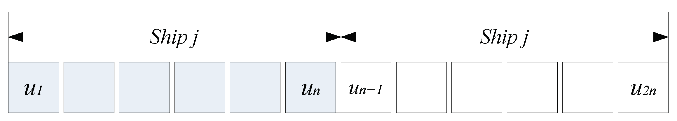
4.1.1. Chromosome Representation

Figure 3 illustrates the chromosome for a GA approach. The chromosome includes two segments, each containing n genes, where n is the total number of ships to call within the planning horizon. In the left segment, the jth gene is an integer indicating the berth number assigned to the ship j; in the right segment the jth is an integer representing the number of QCs assigned to the ship j. The two segments together indicate a total solution to the simultaneous DDBAP and DQCAP.

4.1.2. Population Initialization

Given a total number of chromosomes, the GA generates integers within [1,m] for the left segment as well as integers within [$r^{min},r^{max}$] for the right segment of a chromosome iteratively in these chromosomes.

4.1.3. Population Reproduction

The proposed GA employs roulette wheel selection (RWS) for population reproduction. Equation (13) is the formula used to calculate the selection probability for each chromosome, in which $F{V}_i$ indicates the fitness value of the chromosome i. In addition, Equation (14) shows the calculation of cumulative probability for each chromosome. The RWS sampling allows the best chromosomes with a higher opportunity to be selected as parents for generating offspring.

$$p_i=\frac{F{V}_i}{{{\displaystyle \sum }}_{i=1}^{n}F{V}_i}$$

(13)

$$C{p}_n={{\displaystyle \sum }}_{i=1}^n{p}_i, n = 1, \dots , P$$

(14)

4.1.4. Crossover Operation

The crossover operator is used to generate offspring chromosomes. It works as follows. As shown in Figure 4a, it selects two points (p1 and p2) as a matching section from two parent chromosomes (A and B). Then, it switches all the elements in the matching section between the two parent chromosomes. After crossover operation, it results in two offspring chromosomes (A₁ and B₁) as shown in Figure 4b.

4.1.5. Mutation Operation

Mutation operation can be used to diversify a population to prevent a solution from being trapped in local optima. A mutation is bound by a specified mutation rate (Rm); if a selected random number from the range [0,1] is equal or smaller than the Rm then the mutation triggers. In this research, three kinds of mutation operators are focused and they are detailed below.

(1)

Swap mutation (SWM): as shown in Figure 5a, two genes located at the positions p1 and p2 of a same segment are select and swapped. Thus, the chromosome A mutates to A2 as shown in Figure 5b.

(2)

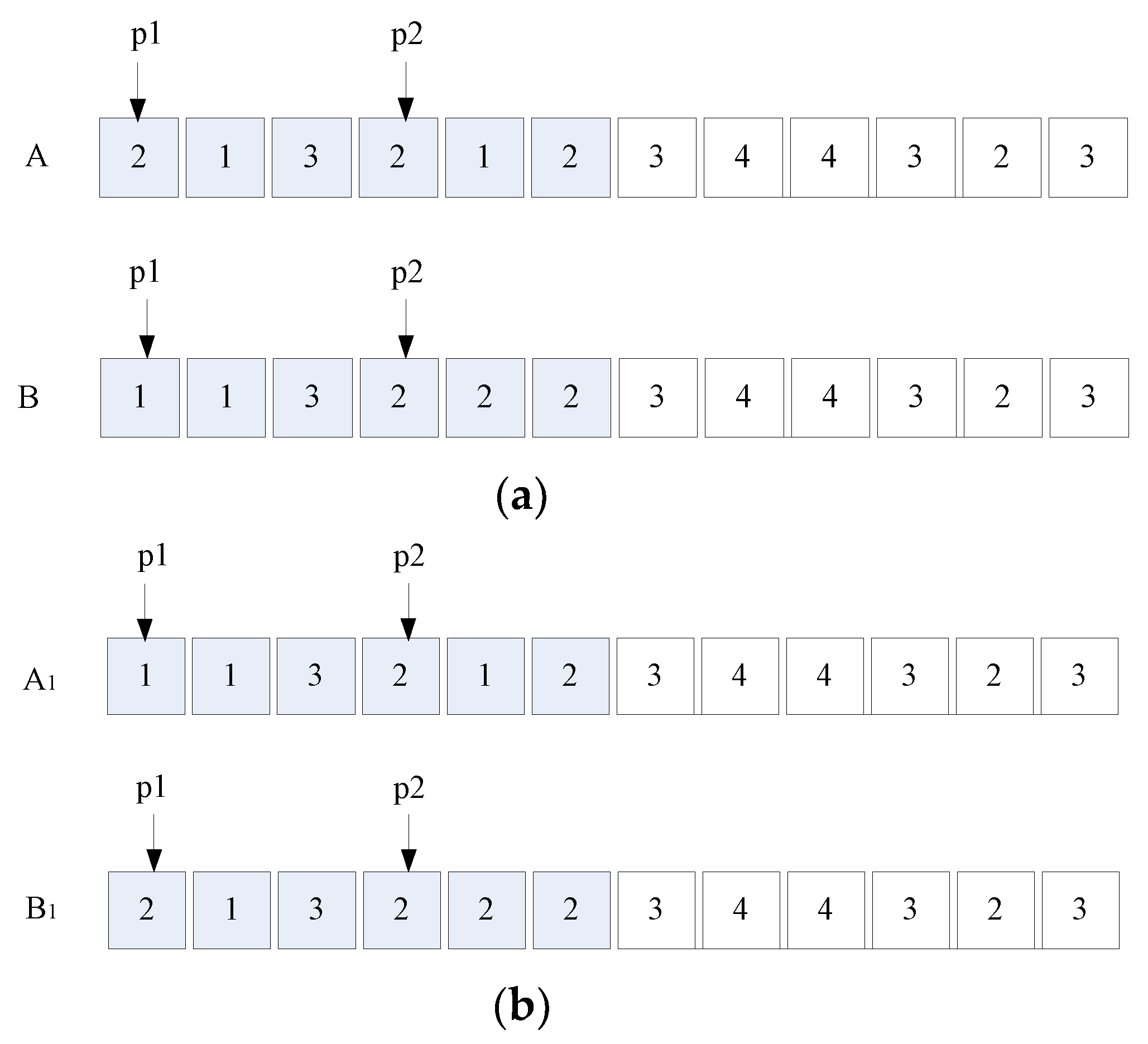
Thoros mutation: as shown in Figure 6a, three gene positions p1 < p2 < p3 are chosen randomly, which shall take the different positions not necessarily successively. Then, the gene value of position p1 becomes the gene value of position p2, the original gene value of p2 becomes the gene value of p3, and finally the original gene value of p3 becomes the gene value of p1. After mutation, Figure 6a becomes Figure 6b.

(3)

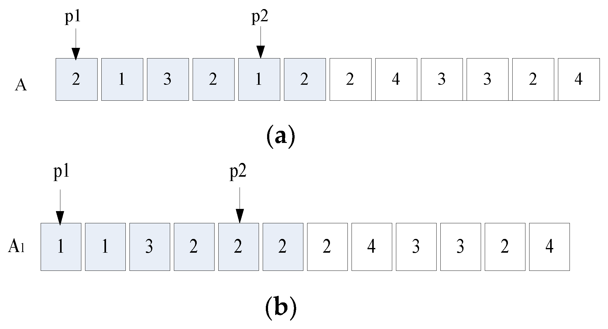
Thoras mutation: as shown in Figure 7a, the process of Thoras mutation is similar that of Thoros mutation. But the Thoras selects three consecutive genes. After randomly selecting the first gene position (p1), the two other successive genes are then determined. As a result, the last becomes the first of the sequence, the second becomes last and the first becomes the second in the sequence. After mutation, the Figure 7a becomes Figure 7b. Each mutation is subject to constraints, Equations (10) and (11). For an infeasible solution, it is discarded and regenerated.

4.1.6. Termination

A termination condition is used to stop running a GA within an acceptable computational time. In this research, a number of total generations determined by a preliminary test of convergence is used as a terminate condition.

4.1.7. Fitness Value Function

To evaluate the derived solutions, Equation (15) is defined as the fitness value (FV) function. The higher the FV, the better the solution is. Multiplication of 1000 is used to shift a decimal point for better presentation in a table, and this will not alter the comparative results of different approaches:

$$\mathrm{FV}= \left(1/Z\right)\times 1000$$

(15)

4.1.8. The Whole Process Flow of the HGA Approaches

The main process flow of the HGAs is outlined as follows.

(1)

Set the population size (P) crossover rate (Rm), mutation rate (Rc), the maximum number of generation g_m, and set the current generation i to 1 (I = 1).

(2)

Initiate a population of chromosomes.

(3)

Determine the service priority for each ship.

(4)

If $i=1$ then go to Step (6); otherwise, go to Step (5).

(5)

Population reproduction.

(6)

Crossover operation.

(7)

Mutation operation using SWM/THOROS/THORAS.

(8)

Transform each chromosome in the population into a berth plan.

(8.1)

Sort the estimated times of arrival (ETAs) of those ships assigned to a same berth. Break a tie by ship priority.

(8.2)

Determine the BT_j of each ship.

(8.3)

Determine the ECT_j of each ship using Equation (5).

(9)

Calculate the FV of the current solution and compare it to the best solution; if better then update the best solution.

(10)

Check if the termination condition ($i>$ gm) is met. If “yes” then output the best solution; otherwise, i = i + 1 and go to step (4).

4.2. A Heuristic-Based Event

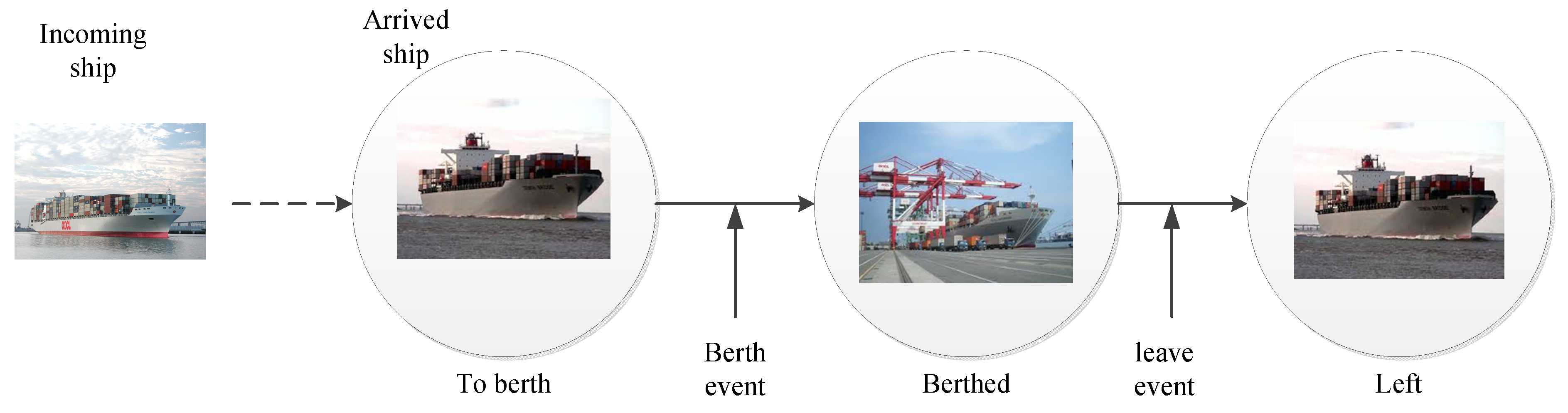
4.2.1. States and Events

In this research, a “state” is defined as a status of a ship and an “event” is defined as thing happens at a specific point of time and this event can change the state of a ship. In this research, we define “to berth,” “berthed,” and “left” as three states of ships and “berth” and “leave” as two events. Figure 8 illustrates a state transition diagram. First, a ship is with the “to berth” state. Then, the “to berth” state can be changed to the “berthed” state triggered by a “berth” event. Finally, the “berthed” state can be changed to “left” state triggered by a “leave” event. The current states of all calling ships can represent a “system” state that can be used to control the running of the event-based heuristic. If all calling ships are with the “left” state, this indicates that all calling ships have been completed so that the event-based heuristic should stop running. The events are also used to trigger QC assignments or reassignments in our approach.

4.2.2. Event-Triggered QC Assignment/Reassignment

Figure 9 illustrates berthing plan that includes variable QC assignment, in which each time interval is termed a “stage” formed by a pair of “berth” and “leave” events. For n ships to call, there will be 2n − 1 stages. Each stage is a time period denoted as [t($\epsilon$), t($\epsilon$ + 1)], where t($\epsilon$) and t($\epsilon$ + 1) correspond to event times of E($\epsilon$) and E($\epsilon$ + 1), respectively. QCs are assigned to each stage to work for ships. Also, note that in this berth plan one employs “leave” events to trigger QC reassignments when QCs are released from finished ships. For example, the “leave” event E(4) of ship 1 reassigns 1 QC (released by ship 1) to ships 2 and 3, respectively. This reassignment should be subject to constraints including Equations (9) and (10). Due to the immediate reuse of released QCs, a higher QC utilization is expected but at the cost of more QC setups and movements. The gains and costs should be justified by in the objective function. In this research, only the “leave” events of ships are used to trigger QC reassignments.

4.2.3. Finding the Next Event

To generate a berth plan based on events, it is necessary to identify time, type and owner of the next event one by one. For this purpose, Equation (14) is used to find the next event time at the stage $\epsilon$, denoted as $t\left(\epsilon \right)$. The $t\left(\epsilon \right)$ is the minimum value of the two data sets, i.e., $\left\{a_j\right|j\in A\}$ and {$EC{T}_j\left(\epsilon -1\right)| j\in B\}$. The $a_j$ is the ETA of a ship j if $j\in A$, werhe A is the set of ships to berth; the $EC{T}_j\left(\epsilon -1\right)$ is the expected completion time of a berthed ship j if $j\in B$, where B is a set of berthed ships. Also note that the $EC{T}_j\left(\epsilon -1\right)$ is estimated at the stage $\epsilon -1$. Break a tie by ship priority. Having found the $t\left(\epsilon \right)$, then the type and owner of the next event can be determined accordingly. If the owner is (ship $j)\in A$, then the next event is a “to berth” event; otherwise, a “leave” type due to $j\in B$.

$$t\left(\epsilon \right) = \{\begin{array}{c}\mathrm{Min}\left\{\underset{j\in A}{\mathrm{Min}}\{a_j\}\right\} ,\epsilon =1\\ \mathrm{Min}\left\{\underset{j\in A}{\mathrm{Min}}\{a_j\}, \underset{j\in B}{\mathrm{Min}}\{EC{T}_j\left(\epsilon -1\right)\}\right\} , \epsilon >1\end{array}$$

(16)

Also, Equation (16) is subject to the following constraints in Equation (17):

$$1<\epsilon \le 2n-1;1\le j\le n; A{\displaystyle \cup }B{\displaystyle \cup }F=\left\{1,\dots ,n\right\}$$

(17)

where

• $n$: the total number of ships.
• $A$: a set of ships at “to berth” state.
• $B$: a set of ships at “berthed” state.
• $F$: a set of ships at “left” state.
• $\epsilon$: the current stage number.
• $EC{T}_j\left(\epsilon -1\right)$: the expected completion time (ECT) of ship j ($j\in B$) estimated at the previous stage $\epsilon -1$.
• $a_j$: the ETA of ship j ($j\in A$).

For a berthed ship j, we can estimate its $EC{T}_j$ using Equation (4). However, this needs to update the $EC{T}_j$ for a ship j if the number of QCs assigned to it has been further changed. Equation (18) is the equation for updating the $ET{C}_j\left(\epsilon \right)$ at the time point $\epsilon$:

$$\begin{array}{ll}ET{C}_j\left(\epsilon \right)& =t\left(\epsilon \right)+(T_{sm}^j\left(\epsilon \right) +\left[\frac{\left(1+\beta ·∆b_j\right)·{\theta }_{\epsilon j}}{{\left(r_{\epsilon j}\right)}^{\alpha }\rho }\right])\\ & = t\left(\epsilon \right)+(T_{sm}^j\left(\epsilon \right) +\left[\frac{\left(1+\beta ·∆b_j\right)}{{\left(r_{\epsilon j}\right)}^{\alpha }\rho }· \frac{\left(ET{C}_j\left(\epsilon -1\right)-t\left(\epsilon \right)-T_{sm}^j\left(\epsilon -1 \right)\right){\left(r_{\left(\epsilon -1\right)j}\right)}^{\alpha }\rho }{\left(1+\beta ·∆b_j\right)}\right])\\ & = t\left(\epsilon \right)+(T_{sm}^j\left(\epsilon \right) +\left[ \frac{\left(ET{C}_j\left(\epsilon -1\right)-t\left(\epsilon \right)-T_{sm}^j\left(\epsilon -1 \right)\right){\left(r_{\left(\epsilon -1\right)j}\right)}^{\alpha }}{{\left(r_{\epsilon j}\right)}^{\alpha }}\right])\end{array}$$

(18)

where:

• $r_{\left(\epsilon -1\right)j}$: the amount of QCs assigned to the ship j at the previous stage $\epsilon -1$
• $r_{\epsilon j}$: the amount of QCs assigned to the ship j at the current stage $\epsilon$

4.2.4. The Event-Based Heuristic for Variable QC Assignment

Equation (19) is proposed to assign/reassign released QCs from a leaving ship to berthed ship(s).

$$r_{\epsilon j}=\{\begin{array}{c}\mathrm{Max}\left\{r^{min},q_j+\mathrm{QUO}\left(\frac{{\theta }_{\epsilon j}}{{{\displaystyle \sum }}_{j\in B}{\theta }_{\epsilon j}}\ast q_{j^{\prime }}\right)\right\}, \mathrm{if} q_j+\mathrm{QUO}\left(\frac{{\theta }_{\epsilon j}}{{{\displaystyle \sum }}_{j\in B}{\theta }_{\epsilon j}}\ast q_{j^{\prime }}\right)\le r^{max}\\ r^{max}, \mathrm{if} q_j+\mathrm{QUO}\left(\frac{{\theta }_{\epsilon j}\left(\epsilon \right)}{{{\displaystyle \sum }}_{j\in B}{\theta }_{\epsilon j}}\ast q_{j^{\prime }}\right)>r^{max}\end{array}$$

(19)

where

• ${\theta }_{\epsilon j}$: is the remaining workload (the total number of containers) of berthed ship j estimated at the stage $\epsilon$.
• $q_j$: is the number of QCs assigned to the berthed ship j.
• $q_{j^{\prime }}$: is the number of QCs released by leaving ship $j^{\prime }$.

4.2.5. The Main Process Flow of the Event-Based Heuristic

The main process flow of the event-based heuristic for generating a series of stage solutions to the DQCAP is outlined in

Table 1. The main flow of the event-based heuristic.

1	Set $\epsilon$ = 1, B = $\varnothing$, F = $\varnothing$, A = $\left\{1,\dots ,n\right\}$
2	While (F $\ne \left\{1,\dots ,n\right\}$) then
3	do{
4	determine the next event time t($\epsilon$) using Equation (16) and identify the owner (ship j) of the next event
5
6	if $\left(\mathrm{ship} j\in A\right)$ then
7	trigger the “berth” event
8	move the ship j from set A to set
9	assign the number of QCs to the ship j ($j\in B$) according to the jth gene value (derived from GA1) in the right segment of the chromosome.
10
11	else if $\left(\mathrm{ship} j\in B\right)$ then
12	trigger the “leave” event
13	move the ship j from set B to set F
14	reassign released QCs from ship j to remaining berthed ships $j^{,}$ ($j^{,}\in B$) using Equation (19)
15
16	update $EC{T}_{j^{,}}\left(\epsilon \right)$ for berthed ships $j^{,}$ ($j^{,}\in B)$ using Equation (18)
17	End if
18	$\epsilon$ = $\epsilon$ + 1
19	}

. Initially, all calling ships (j = 1, …, n) are staying in set A and they will be finally moved to the set F, then this algorithm stops running.

4.3. The Main Process Flow of HGAs

The main process flow of HGAs is outlined as follows.

(1)

Set the population size (P) crossover rate (Rm), mutation rate (Rc), the maximum number of generations gm, and set the current generation i to 1 (i = 1).

(2)

Initiate a population of chromosomes.

(3)

Determine the service priority for each ship.

(4)

If $i=1$ then go to Step (6); otherwise, go to Step (5).

(5)

Population reproduction.

(6)

Crossover operation (TPX).

(7)

Mutation operation (Swap/Thoras/Thoros).

(8)

Transform each chromosome in the population into a berth plan.

(9)

Calculate the FV of the current solution and compare it to the best solution; if better then update the best solution.

(10)

Check if the termination condition ($i>$ gm) is met. If “yes” then output the best solution; otherwise, i = i + 1 and go to step (4).

5. Numerical Example

Java 2 is used as the programming language and experiments are conducted on a PC equipped with an Intel Pentium 2.4 GHz CPU as well as 4G DRAM.

5.1. Parameter Setting and Ship Data Generation for the Example

In our experiments, the parameter settings, m = 3, n = 20, q = 8, $\alpha$ = 0.8, $\beta$ = 0.3, $\rho$ = 25 (containers/hour), $t_s$ = 0.15 (hour), $t_m$ = 0.25 (hour), Rc = 0.4, Rm = 0.5, P = 20 and g_m = 500 and [$r^{min},r^{max}$] = [1,3] are used. The cost rates of $c1, c2 \mathrm{and} c3$ are set to 1000 USD/hour, same to those used in [29]. The ETA ($a_j$) and total number of containers to be handled for a ship j (${\theta }_j$) are randomly values taken from the ranges [0, 168] (hours) and [1, 700] (Twenty-foot Equivalent Units; TEUs), respectively. After this, the program continues to generate ship priority (p_j), desired berth location (b_j) and expected time of departure (ETD_j) that is defined in Equation (11). The values of b_j (j = 1, …, n) are randomly selected from the set of berths [1,m]. The ETD_j (j = 1, …, n) is an optimistic departure time due to the use of $r^{max}$ in Equation (20).

$$ET{D}_j=a_j+\left[\frac{\left(1+\beta ·∆b_j\right)·{\theta }_j}{{\left(r^{max}\right)}^{\alpha }\rho }\right]$$

(20)

5.2. Comparison of Various GAs and HGAs

This section compares results obtained from HGA1, HGA2 and HGA3. Each HGA differs from each other by using a specific mutation operation, i.e., HGA1 uses Swap mutation, HGA2 uses Thoros mutation and HGA3 uses Thoras mutation.

Table 2. The experimental results obtained from the GAs and HGAs.

	(1) GA1 FV	(2) GA1 Time	(3) HGA1 FV	(4) HGA1 Time	(5) GA2 FV	(6) GA2 Time	(7) HGA2 FV	(8) HGA2 Time	(9) GA3 FV	(10) GA3 Time	(11) HGA3 FV	(12) HGA3 Time
20 × 3	1.939	120.0	2.341	8.4	2.057	111.0	2.257	8.4	1.954	108.0	2.195	9.0
	1.789	111.0	2.187	8.1	2.261	108.0	2.553	9.0	1.987	108.0	2.255	8.1
	1.729	111.0	2.044	8.4	2.257	111.0	2.461	8.1	2.048	111.0	2.321	8.4
	2.473	120.0	2.503	8.4	2.152	111.0	2.525	8.1	2.314	111.0	2.809	9.0
	2.134	111.0	2.457	8.7	2.112	108.0	2.623	8.4	1.815	111.0	2.618	8.4
	1.656	111.0	2.035	8.1	2.098	111.0	2.294	8.4	1.702	120.0	2.317	9.6
	1.964	111.0	2.461	8.1	1.902	111.0	2.407	8.4	2.512	108.0	2.602	8.4
	2.126	108.0	2.390	8.1	1.974	111.0	2.458	8.4	1.901	111.0	2.092	8.4
	2.572	111.0	2.781	8.4	1.917	111.0	2.379	8.3	2.361	108.0	2.607	8.4
	1.541	111.0	2.136	8.4	1.912	111.0	2.483	8.1	2.253	111.0	2.484	8.4
Average	1.992	112.5	2.334	8.3	2.064	110.4	2.444	8.4	2.085	110.7	2.430	8.6
40 × 3	0.950	210.0	1.394	22.5	0.946	231.0	1.127	22.8	0.759	217.5	1.169	21.0
	0.703	216.0	1.024	21.0	0.455	216.0	0.877	21.9	0.861	216.6	1.283	21.0
	0.484	216.0	0.747	21.9	0.750	201.9	1.134	21.6	0.819	216.9	1.316	21.0
	0.675	222.0	1.135	21.6	0.584	216.9	1.231	21.6	0.814	219.6	2.227	21.0
	0.751	216.0	1.212	21.6	0.691	215.4	1.095	20.7	0.790	216.0	1.069	21.0
	0.775	216.0	1.335	21.3	0.602	219.3	0.907	22.2	0.751	216.9	0.933	21.0
	0.395	219.0	0.779	22.2	0.657	222.3	0.862	21.9	0.716	218.1	1.112	24.0
	0.807	216.0	1.327	21.0	0.722	219.0	1.027	22.8	0.605	219.0	1.091	21.0
	0.763	225.0	1.006	21.9	1.075	228.0	1.506	24.0	0.550	225.0	0.770	24.0
	0.691	222.0	1.308	23.4	0.685	231.0	1.708	21.0	0.677	222.0	1.381	24.0
Average	0.699	217.8	1.127	21.8	0.717	220.1	1.147	22.1	0.734	218.8	1.235	21.9
60 × 3	0.124	315.0	0.253	39.0	0.137	303.0	0.322	126.0	0.143	303.0	0.390	39.0
	0.136	306.0	0.418	42.0	0.156	306.0	0.340	42.0	0.209	501.0	0.399	42.0
	0.164	339.0	0.316	39.0	0.227	318.0	0.482	45.0	0.217	381.0	0.523	42.0
	0.125	348.0	0.242	42.0	0.298	321.0	0.545	39.0	0.382	315.0	0.662	36.0
	0.135	315.0	0.267	51.0	0.222	303.0	0.424	39.0	0.222	303.0	0.374	39.0
	0.201	300.0	0.475	39.0	0.217	300.0	0.444	39.0	0.156	303.0	0.449	39.0
	0.201	300.0	0.259	39.0	0.138	300.0	0.277	39.0	0.202	303.0	0.457	42.0
	0.182	333.0	0.397	39.0	0.141	303.0	0.317	39.0	0.197	282.0	0.399	42.0
	0.109	303.0	0.275	45.0	0.158	303.0	0.402	39.0	0.183	303.0	0.461	42.0
	0.133	354.0	0.365	48.0	0.178	306.0	0.400	39.0	0.169	288.0	0.523	51.0
Average	0.151	321.3	0.327	42.3	0.187	306.3	0.395	48.6	0.208	328.2	0.464	41.4
80 × 3	0.101	417.0	0.247	66.0	0.071	411.0	0.213	66.0	0.071	417.0	0.166	66.0
	0.069	414.0	0.136	66.0	0.084	405.0	0.166	66.0	0.069	420.0	0.137	66.0
	0.062	417.0	0.115	66.0	0.078	414.0	0.198	66.0	0.065	384.0	0.118	66.0
	0.090	390.0	0.222	66.0	0.079	420.0	0.168	66.0	0.083	414.0	0.170	66.0
	0.069	411.0	0.121	66.0	0.082	414.0	0.169	66.0	0.088	390.0	0.145	66.0
	0.082	414.0	0.122	66.0	0.076	402.0	0.161	66.0	0.085	402.0	0.250	66.0
	0.054	417.0	0.158	66.0	0.064	417.0	0.151	66.0	0.073	414.0	0.169	66.0
	0.078	408.0	0.137	66.0	0.073	414.0	0.177	66.0	0.077	423.0	0.182	66.0
	0.080	411.0	0.156	69.0	0.057	414.0	0.119	66.0	0.064	411.0	0.146	69.0
	0.086	414.0	0.137	69.0	0.079	366.0	0.110	57.0	0.077	555.0	0.192	63.0
Average	0.077	411.3	0.155	66.6	0.074	407.7	0.163	65.1	0.075	423.0	0.168	66.0
100 × 3	0.039	453.0	0.077	87.0	0.041	453.0	0.090	87.0	0.048	459.0	0.131	87.0
	0.036	453.0	0.060	87.0	0.036	444.0	0.070	93.0	0.041	462.0	0.097	87.0
	0.040	462.0	0.091	87.0	0.039	462.0	0.093	87.0	0.040	462.0	0.081	90.0
	0.043	462.0	0.093	87.0	0.046	459.0	0.095	87.0	0.037	450.0	0.091	90.0
	0.032	447.0	0.072	87.0	0.046	450.0	0.113	87.0	0.034	471.0	0.069	90.0
	0.035	444.0	0.075	93.0	0.030	456.0	0.058	87.0	0.037	459.0	0.080	96.0
	0.036	456.0	0.098	90.0	0.042	486.0	0.086	90.0	0.035	552.0	0.065	99.0
	0.043	471.0	0.094	90.0	0.041	447.0	0.079	102.0	0.058	486.0	0.112	87.0
	0.036	462.0	0.070	87.0	0.043	456.0	0.109	87.0	0.039	453.0	0.085	87.0
	0.035	462.0	0.076	93.0	0.036	453.0	0.072	84.0	0.039	441.0	0.100	96.0
Average	0.038	457.2	0.081	88.8	0.040	456.6	0.086	89.1	0.041	469.5	0.091	90.9

Illustrates the FVs and average FVs obtained from various GAs and HGAs at different problem sizes. The higher the FV the better the goodness of an approach.

Figure 10 depicts average FVs obtained from the three GAs with time-invariant QC assignment at differ problem sizes of n × 3 (with n = 20, 40, 60, 80 and 100). The average FV shows a downward trend when more ships are calling at the port. It is found that GA1 has the worst average FV; GA2 has the second best average FV; the GA3 has the best average FV.

Figure 11 depicts the graph of average FVs obtained from the three HGAs with variable QC assignment at different problem sizes of n × 3 (with n = 20, 40, 60, 80 and 100). The average FV shows a downward trend when more ships are calling at the port. Also, among the three HGAs, it is found that HGA1 has the worst average FVs; HGA2 has the second best average FV; and HGA3 has the best average FV.

Figure 12 shows the improvements of average FVs obtained from different HGAs with different mutation operations at different problem sizes if n × 3 (n = 20, 40, 60, 80 and 100), compared to traditional GAs used for time-invariant QC assignments. We analyze this figure in the next section.

5.3. Findings and Discussion

The findings and discussion are as follows:

(1)

Our experimental results showed that the three HGAs can generate variable QC assignments and the derived results are better than those obtained from a GA with time-invariant QC assignment.

(2)

Figure 12 shows the average advantages percentage obtained from the three HGAs compared with GAs under different problem sizes. Generally speaking, the larger the problem size, the greater the advantage. Compared with GA3, HGA3 has the best advantage (123.3%) at the problem size 100 × 3.

(3)

Different mutation operations employed by a GA or HGA can lead to different planning results. In terms of average FV, our experiments showed that the GA3 with Thoros mutation had the best performance; the GA2 with Thoras is the second best; the GA1 with Swap mutation is the worst. Compared with the two-point mutation operation Swap, the three-point mutation operations including Thoras and Thoros appear to be more capable of exploring a solution space.

(4)

The variable QC assignment can lead to advantages for these HGAs. This kind of QC assignment can reassign released QCs immediately to other ships, which can reduce the handling time for ships due to increased QC capability. Furthermore, the reduced handling times of ships can lead to an earlier release of berth and thus waiting times and then delay times of ships. This initiates a positive chain effect.

(5)

In this research the gain from the variable QC assignment has been justified against the cost of more QC setups and movements.

(6)

Among the three proposed HGAs, our experiments showed that the HGA3 had the best performance in terms of average FV.

(7)

The average computational times required for HGAs to complete experimental runs at different problem sizes n × 3 (with n = 20, 40, 60, 80 to 100) are acceptable. For example, at the problem size 100 × 3 an average of 469.5 + 90.9 s (or about 9 min) are required for HGA3 to complete one experiment when setting n = 100 and iteration runs = 500.

6. Conclusions

DDBAP and DQCAP are two daily seaside operational problems faced by container teminal planners. To better utilize berths and QCs, a better way to cope with the two problems simultaneously is necessary.

Although GAs have been widely used to cope with the DDBAP and DQCAP, however, almost all of them have been used to perform time-invariant QC assignment. Due to the lack of flexibility, this cannot best utilize available QCs. In addition, in past study, fixed-time interval planning framework has been widely used. This kind of framework has the disadvantage of underutilizing available QC capability. To address this issue, in this research the variable-time interval planning framework has been proposed for HGAs. Each of the three HGA combines GA with an event-based heuristic to solve the DDBAP and DQCAP simultaneously. The experiments gave a good result. We highlight the contributions of this research as follows.

(1)

Three novel HGAs have been proposed to cope with the DDBAP and DQCAP simultaneously. Each of the three HGAs combines a GA with an event-based heuristic. The dynamic framework embedded in these HGAs enables variable QC assignment that can better utilize available QCs.

(2)

Our experiment results showed that the HGAs with variable QC assignments can outperform those GAs with time-invariant QC assignment. Also, it is found that the HGA3 had the best performance among the three HGAs.

(3)

In this research we have proposed Equation (1) to estimate the handling time for ships, with the handling time also include required times for QC setup and movements. In addition, in the objective function the costs of QC setup and movement have been included, which helps to justify the gains from the flexibility of QC reassignments.

(4)

The HGAs appear to be applicable for berth allocation and QC assignment for calling ships due to acceptable computational time.

(5)

The research compares time-invariant QC assignment with variable QC assignment. These kinds of studies have been rarely undertaken in the past.

In this research, the HGAs only employ “leave” events to trigger QC assignment/reassignment. The use of “berth” event only or both “leave” and “berth” events and the investigation of their effects can be conducted in future research. In addition, the effects of using different crossover operations for the HGAs can be investigated. Moreover, hybrid approaches combining other meta-heuristics such as artificial bee colony (ABC) and shuffle frog-leaping algorithm (SFLA) can be developed in future research. Extending the HGAs proposed in the research to deal with continuous BAP can be another focus in future research.

References

1. Hsu, H.P.; Wang, C.N.; Chou, C.C.; Lee, Y.; Wen, Y.F. Modeling and Solving the Three Seaside Operational Problems Using an Object-Oriented and Timed Predicate/Transition Net. Appl. Sci. 2017, 7, 218. [Google Scholar] [CrossRef]
2. Vis, I.F.A.; de Koster, R. Transshipment of container at a container terminal: An overview. Eur. J. Oper. Res. 2003, 147, S0377–S2217. [Google Scholar] [CrossRef]
3. Salido, M.A.; Mario, R.M.; Barber, F. A decision support system for managing combinatorial problems in a container terminal. Knowl. Based Syst. 2012, 29, 63–74. [Google Scholar] [CrossRef]
4. Bierwirth, C.; Meisel, F. A follow-up survey of berth allocation and quay crane scheduling problems in container terminal. Eur. J. Oper. Res. 2015, 244, 675–689. [Google Scholar] [CrossRef]
5. Liang, C.J.; Huang, Y.F.; Yang, Y. A quay crane dynamic scheduling problem by hybrid evolutionary algorithm for berth allocation planning. Comput. Ind. Eng. 2009, 56, 1021–1028. [Google Scholar] [CrossRef]
6. Raa, B.; Dullaert, W.; Schaeren, R.V. An enriched model for the integrated berth allocation and quay crane assignment problem. Expert Syst. Appl. 2011, 38, 4136–4147. [Google Scholar] [CrossRef]
7. Zhang, C.R.; Zheng, L.; Zhang, Z.H.; Shi, L.Y.; Armstrong, A.J. The allocation of berths and quay cranes by using a sub-gradient optimization technique. Comput. Ind. Eng. 2010, 58, 40–50. [Google Scholar] [CrossRef]
8. Bierwirth, C.; Meisel, F. A survey of berth allocation and quay crane scheduling problems in container terminals. Eur. J. Oper. Res. 2010, 202, 615–627. [Google Scholar] [CrossRef]
9. Imai, A.; Chen, H.C.; Nishimura, E.; Papadimitriou, S. The simultaneous berth and quay crane allocation problem. Transp. Res. Part E Logist. Transp. Rev. 2008, 5, 900–920. [Google Scholar] [CrossRef]
10. Zhou, P.F.; Kang, H.G. Study on berth and quay-crane allocation under stochastic environments in container terminal. Syst. Eng. Theory Pract. 2008, 28, 161–169. [Google Scholar] [CrossRef]
11. Chang, D.F.; Jiang, Z.H.; Yan, W.; He, J.L. Integrating berth allocation and quay crane assignments. Transp. Res. Part E Logist. Transp. Rev. 2010, 46, 975–990. [Google Scholar] [CrossRef]
12. Han, X.L.; Lu, Z.Q.; Xi, L.F. A proactive approach for simultaneous berth and quay crane scheduling problem with stochastic arrival and handling time. Eur. J. Oper. Res. 2010, 207, 1327–1340. [Google Scholar] [CrossRef]
13. Liang, C.J.; Guo, J.Q.; Yang, Y. Multi-objective hybrid genetic algorithm for quay crane dynamic assignment in birth allocation planning. J. Intell. Manuf. 2011, 22, 471–479. [Google Scholar] [CrossRef]
14. Brown, G.G.; Lawphongpanich, S.; Thurman, K.P. Optimizing ship berthing. Nav. Res. Logist. 1994, 41. [Google Scholar] [CrossRef]
15. Imai, A.; Nagaiwa, K.I.; Tat, C.W. Efficient planning of berth allocation for container terminals in Asia. J. Adv. Transp. 1997, 31, 75–94. [Google Scholar] [CrossRef]
16. Imai, A.; Nishimura, E.; Papadimitrious, S. The dynamic berth allocation problem for a container port. Transp. Res. Part B Methodol. 2001, 35, 401–417. [Google Scholar] [CrossRef] [Green Version]
17. Imai, A.; Nishimura, E.; Papadimitrious, S. Berth allocation with service priority. Transp. Res. Part B Methodol. 2003, 37, 437–457. [Google Scholar] [CrossRef] [Green Version]
18. Hansen, P.; Oǧuz, C.; Mladenović, N. Variable neighborhood search for minimum cost berth allocation. Eur. J. Oper. Res. 2008, 191, 636–649. [Google Scholar] [CrossRef]
19. Golias, M.M.; Boile, M.; Theofanis, S. Service Time Based Customer Differentiation Berth scheduling. Transp. Res. Part E Logist. Transp. Rev. 2009, 45, 878–892. [Google Scholar] [CrossRef]
20. Saharidis, G.K.D.; Golias, M.M.; Boile, M.; Theofanis, S.; Ierapetritou, M.G. The berth scheduling problem with customer differentiation: A new methodological approach based on hierarchical optimization. Int. J. Adv. Manuf. Technol. 2010, 46, 377–393. [Google Scholar] [CrossRef]
21. Xu, D.S.; Li, C.L.; Leung, J.Y.T. Berth allocation with time-dependent physical limitations on vessels. Eur. J. Oper. Res. 2012, 216, 47–56. [Google Scholar] [CrossRef]
22. Lalla-Ruiz, E.; Expósito-Izquierdo, C.; Melián-Batista, B.; Moreno-Vega, J.M. A set-partitioning-based model for the berth allocation problem under time-dependent limitations. Eur. J. Oper. Res. 2016, 250, 1001–1012. [Google Scholar] [CrossRef]
23. Ursavas, E.; Zhu, S.X. Optimal policies for the berth allocation problem under stochastic nature. Eur. J. Oper. Res. 2016, 255, 380–387. [Google Scholar] [CrossRef]
24. Dulebenets, M.A. A novel Memetic Algorithm with a deterministic parameter control for efficient berth scheduling at marine container terminals. Marit. Bus. Rev. 2017, 2, 302–330. [Google Scholar] [CrossRef]
25. Umang, N.; Bierlaire, M.; Erera, A.L. Real-time management of berth allocation with stochastic arrival and handling times. J. Sched. 2017, 20, 67–83. [Google Scholar] [CrossRef]
26. Zhen, L.; Liang, Z.; Zhuge, D.; Lee, L.H.; Chew, E.P. Daily berth planning in a tidal port with channel flow control. Transp. Res. Part B Methodol. 2017, 106, 193–217. [Google Scholar] [CrossRef]
27. Dulebenets, M.A. Application of Evolutionary Computation for berth scheduling at marine container terminals: Parameter tuning versus parameter control. IEEE Trans. Intell. Transp. Syst. 2018, 19, 25–37. [Google Scholar] [CrossRef]
28. Dulebenets, M.A.; Kavoosi, M.; Abioye, O.; Pasha, J. A Self-Adaptive Evolutionary Algorithm for the Berth Scheduling Problem: Towards Efficient Parameter Control. Algorithms 2018, 11, 100. [Google Scholar] [CrossRef]
29. Giallombardo, G.; Moccia, L.; Salani, M.; Vacca, I. Modeling and solving the tactical berth allocation problem. Transp. Res. Part B Methodol. 2010, 44, 232–245. [Google Scholar] [CrossRef]
30. Li, M.W.; Hong, W.C.; Geng, J.; Wang, J. Berth and quay crane coordinated scheduling using multi-objective chaos cloud particle swarm optimization algorithm. Neural Comput. Appl. 2017, 28, 3163–3182. [Google Scholar] [CrossRef]
31. Xiang, X.; Liu, C.; Miao, L. Reactive strategy for discrete berth allocation and quay crane assignment problems under uncertainty. Comput. Ind. Eng. 2018, 126, 196–216. [Google Scholar] [CrossRef]
32. Meisel, F.; Bierwirth, C. Heuristic for the integration of crane productivity in the berth allocation problem. Transp. Res. Part E Logist. Transp. Rev. 2009, 45, 196–209. [Google Scholar] [CrossRef]
Figure 1. (a). A berth plan with time-invariant quay crane (QC) assignment. (b). A berth plan with variable QC assignment.
Sustainability 11 02018 g001
Figure 2. The procedure of hybrid genetic algorithms (HGAs).
Sustainability 11 02018 g002
Figure 3. The chromosome representation of a genetic algorithm (GA).
Sustainability 11 02018 g003
Figure 4. (a). Two chromosomes before crossover operation. (b) Two chromosomes after crossover operation.
Sustainability 11 02018 g004
Figure 5. (a). Chromosome A before swap mutation operation. (b) Chromosome A after swap mutation operation.
Sustainability 11 02018 g005
Figure 6. (a). Before Thoros mutation operation. (b) After Thoros mutation operation.
Sustainability 11 02018 g006
Figure 7. (a). Before Thoras mutation operation. (b) After Thoras mutation operation.
Sustainability 11 02018 g007
Figure 8. The states and events defined in this research.
Sustainability 11 02018 g008
Figure 9. The berth plan with variable QC assignment triggered by a “leave” event.
Sustainability 11 02018 g009
Figure 10. The average FVs obtained from GAs with time-invariant QC assignment at different problem sizes n × 3 (with n = 20, 40 to 100).
Sustainability 11 02018 g010
Figure 11. The average FVs obtained from HGAs with variable QC assignment at different problem sizes n × 3 (with n = 20, 40 to 100).
Sustainability 11 02018 g011
Figure 12. The improvements of average FVs obtained from different HGAs at different problem size n × 3 (with n = 20, 40 to 100).
Sustainability 11 02018 g012