Article

Development of an Event-Based Water Quality Model for Sparsely Gauged Catchments

1
Institute for Computational Science and Technology, Ho Chi Minh City 700000, Vietnam
2
Center of Water Management and Climate Change, Vietnam National University, Ho Chi Minh City 700000, Vietnam
3
Leichtweiss-Institute for Hydraulic Engineering and Water Resources, University of Braunschweig, 38106 Braunschweig, Germany
4
Department of Civil and Environmental Engineering, Seoul National University, Seoul 08826, Korea
*
Author to whom correspondence should be addressed.
Sustainability 2019, 11(6), 1773; https://doi.org/10.3390/su11061773
Submission received: 28 February 2019 / Revised: 19 March 2019 / Accepted: 20 March 2019 / Published: 24 March 2019

Abstract

:
This paper describes an event-based water quality model for sparsely gauged catchments. The model was cultivated in a robust way to cope with practical issues, such as limited available data and error propagation. A simplified model structure and fewer input parameters are the most appealing features of this model. All model components are coupled and controlled within an Excel Spreadsheet Macro as an operational tool. Herein, the geomorphological instantaneous unit hydrograph (GIUH), the simplified process erosion and sedimentation component, the loading function, and the river routing from different existing modeling systems are adopted and linked together. Furthermore, an add-on Monte Carlo simulation tool is provided to deliver an uncertainty analysis for calibration of the output obtained from the model results. The model was successfully applied to simulate nutrient dynamics for small catchment scales during flood events in Vietnam. The success of the model application shows the ability of our model, which can adapt the model complexity to the data availability, i.e., the dominant processes in the system should be captured, whereas the minor processes may be neglected or treated in a less complex manner.

1. Introduction

Water pollution is a critical water-related problem, since it threatens human beings, as well as ecosystems. The excess of nutrients in the aquatic environment is a typical example of water pollution caused by various anthropogenic factors from industrial and urban wastewater, and agricultural runoff. Eutrophication can be seen as a consequence of excessive nutrients, which can lead to serious environmental problems such as limited water supply, severe hypoxia, and polluted aquatic ecosystems. Through the food chain, water pollution can cause serious waterborne diseases to human [1,2,3].
Catchment water quality modeling was shown as a useful tool for water quality management. It is widely applied in several water quality management programs, such as the total maximum daily load (TMDL) estimation in the United States of America (USA) [4], or in the water framework directive in the European community [4]. The physical, chemical, and biological processes occurring in the catchment, as well as the anthropogenic factors, can be included in the model so that various management schemes can be tested and implemented. Therefore, it can be used to assist water managers in giving effective decisions for water management and protection.
There are a wide range of available catchment models [5], whose various characteristics and different applications create a difficult situation for a potential user. Therefore, model selection is a crucial task in order to have a suitable package for a particular area under specific conditions. For example, Borah and Bera [4,6] conducted an extensive review of different catchment water quality models for both event (e.g., agricultural non-point source pollution model (AGNPS), areal nonpoint source watershed environment response simulation (ANSWERS), Dynamic watershed simulation model (DWSM), kinematic runoff and erosion model (KINEROS)) and continuous (e.g., AnnAGNPS, ANSWERS-Continuous, hydrological simulation program—Fortran (HSPF), soil and water assessment tool (SWAT), MIKE système hydrologique Européen (MIKE-SHE)) simulations. They examined model capability, temporal and spatial representation, mathematical strength, and applicability of hydrology, sediment, chemical, and best management practice (BMP) components. In their conclusion, the DWSM model was most suitable for event simulation, and HSPF and SWAT models were best fitted for continuous simulations. Another example is given by the Benchmark project (benchmark models for the water framework directive) [7,8,9], whereby they provided a recommendation and criteria selection of the use and evaluation of models to aid the implementation of the water framework directive (WFD). The most notable results obtained from this project were a model selection protocol [8], benchmark criteria, and a scoring scheme [7,9], which are very helpful for model selection.
Data scarcity is a common problem in the application of catchment modeling. Many catchments are “sparsely gauged” with limited or no observed data for variables required in the application of catchment models. In developing countries, the lack of data is not restricted to any particular area and/or scales (temporal and spatial) [10,11]. The medium frequency of data collection is usually monthly, which practically cannot allow exploring the dynamics of the system during flood events. Therefore, modeling on nutrient dynamics at a small catchment scale during flood events in tropical regions for hourly time-step analysis is still limited. Most models focus on stream flow and sediment dynamics rather than looking at the nutrient variations.
For example, Campling et al. [12] applied the Topographic Hydrologic Model (TOPMODEL) to simulate the relationship between rainfall and runoff; Marsik and Waylen [13] used the CASC2D model to assess the changes of land cover on hydrological processes; Diaz-Ramirez et al. [14] provided an example of utilization of the HSPF model to study hydrology, soil erosion, and sediment transport for tropical island watersheds at a monthly time step. Polyakov et al. [15] applied the AnnAGNPS model to simulate the runoff and sediment in a tropical catchment; however, this study was also limited to daily and monthly time steps. Other studies on nutrient dynamics were based on analyzing sampled data [16,17] in a statistical manner, or applying models at a farm scale.
Most recently, Lorenz et al. [18] applied the ecohydrological PANTA RHEI-WQ model to the catchment of Thi Vai estuary in southern Vietnam. Results were input into the hydrodynamic water quality model DELFT-3D for a detailed simulation of the hydrodynamics and water quality of the estuary system under anthropogenic impact and climate change [19]. Such a combination of models usually requires availability of multi-year, historical, hydrometeorological, and water quality data for model calibration. Therefore, the objective of this study was to develop a new model to simulate nutrient dynamics for sparsely gauged catchments during flood events. For this goal, the new model should be simple and robust, and should include tools for uncertainty analysis in order to capture rapid flooding events in hourly time steps. By combining existing and well-approved process components with a focus on data scarcity and model robustness applicability to the tropics, in addition to utilization by, e.g., environmental agencies rather than research institutions, a new model system was created. Results obtained from an application for flood events of a tropical and sparsely gauged catchment show the potential of our model; it can be applied as a water quality management tool to deal with practical issues such as limited data and model complexity at sparsely gauged catchments.

2. Model Development

A scheme of the water quality model is shown in Figure 1. A catchment was discretized into a number of sub-catchments using a watershed delineation function in a Geographic Information System (GIS) tool. A sub-catchment was considered as a modeling unit for nutrient, sediment load, and transport. The water quality model was mainly connected in four consecutive modules: hydrology, erosion, nutrient loading, and river routing modules. In addition, an uncertainty module using the Monte Carlo method was added to the model in order to deal with the uncertainty of model input parameters. In the sections below, a detailed description for each module is given.

2.1. Hydrology Module

The hydrological module was partly adopted from the previous works of the authors [20], in which the model was verified and applied for several flood events in Vietnam in 2005. In this module, the runoff after storm events is modeled as a total flow discharge of the catchment, then its results are later used to convert from nutrient loads into the concentration at the outlet. Moreover, the runoff generated by this hydrological module is used for both erosion and nutrient components. The geomorphology instantaneous unit hydrograph (GIUH) was first initiated by Rodríguez-Iturbe et al. [21], and restated by Gupta et al. [22]. The GIUH is an empirical event-based model approach that combines easily observable (surface) geomorphologic catchment characteristics with a simple regression analysis. This approach is particularly applicable in data-scarce areas, and the model parameterization relies on GIS-based digital elevation model (DEM) processing [23]. The concept of this approach was improved and successfully implemented as an event-based hydrological model to simulate the rainfall–runoff relationship, and to forecast floods [20,24,25,26]. The GIUH is superior in comparison to the traditional IUH, because the GIUH takes into account nonlinear and linear characteristics and is able to deal with ungagged catchments [21]. Simulation results showed that this approach is a very promising tool to estimate event discharges, even for ungauged catchments [20,27].
Rodríguez-Iturbe and Valdez [21] defined simple empirical relationships for the time to peak (tp) and the instantaneous hydrograph peak (qp) of the GIUH dependent on geomorphologic parameters, as follows:
t p = 0.44 R L 0.38 ( R B R A ) 0.55 ( L Ω v ) ,   [ hour ] ,
q p = 1.31 R L 0.43 ( v L Ω ) ,   [ hour 1 ] ,
where LΩ is the length of the highest order stream (km), v is the expected stream flow velocity (m/s), RB is the bifurcation ratio, RA is the area ratio, and RL is the length ratio (see Appendix Table A4).
In Equations (1) and (2), the geomorphologic parameters (RB, RA, and RL) can be easily extracted from the topological characteristics of the catchment using the GIS tool (see, e.g., Integrated Land and Water Information System, ILWIS) [28]. The flow velocity has to be defined by physical reasoning, where an average velocity must be related to an average flow length (i.e., travel path) and the travel time. Travel time is calculated based on estimated flow velocity and geomorphologic parameters (i.e., drainage density).
The response function of the GIUH is characterized as an “impulse response function” [29,30]. The runoff can be obtained from
Q ( t ) = 0 t i ( τ ) u ( t τ ) d τ ,   [ hour 1 ] ,
where i(τ) is the effective rainfall intensity at time τ, and it is distributed uniformly over entire basin. The amount of input entering the system between τ and τ + is i(τ) . The effective (excess) rainfall is computed according to the Soil Conservation Service (SCS) runoff method [29,30].
Furthermore, u(t) is the GIUH, which is the impulse response function of the system, and it is determined as follows:
u ( t ) = t Prob ( T B t )   or :   u ( t ) = t ( S i Prob ( T S i t ) Prob ( S i ) ) ,
where Prob() is the probability of the set given in parentheses, TB is the travel time to the catchment outlet, TSi is the travel time in a particular path, Prob(Si) is the probability of a drop which will travel all possible paths Si to the outlet, and Prob(TSi) is the probability density function (pdf) of the total path travel time TSi.

2.2. Erosion Module

In this module, soil erosion and sediment transport from sources (upland) to the nearest water body are simulated at an hourly time step. Given the objective of model application for the data-scarce areas, the erosion/sediment component was developed based on a simplified process (SP) model for sediment yield, which was basically adapted from Hartley [31]. The model was tested, and it proved to be suitable for modeling the erosion during (extreme) flood events at hourly time step [32,33]. The model attempts to minimize both data inputs and computational effort while maintaining a relatively high degree of similarity to both hydrologic and hydraulic processes [31]. The erosion model aims to compromise between simple empirical modeling (e.g., Universal Soil Loss Equation (USLE) [34]) and complex physically based approaches (e.g., KNIEROS) [31].
As shown in Figure 1, the sediment supply is basically the sum of sediments detached by runoff and rainfall. The runoff is the only source for the transport of sediment which is represented by the sediment transport capacity. The runoff is calculated from the hydrological component. After comparing between the sediment supply and sediment transport capacity, the smaller value is taken as the sediment yield obtained from the catchment. Results from this module are input into the river routing module.

2.2.1. Sediment Supply

The potential sediment supply caused by rainfall is calculated based on the rainfall energy rate which is used in the USLE method, whereas the sediment caused by runoff is based on the stream power equation.

Sediment Caused by Rainfall

Sediment supply by rainfall [31] is calculated as follows:
G r f = E r f ( 1 G C ) C F K ,
where Grf is the rate of soil detachment due to rainfall (mass rate of detachment per unit area by rainfall) (kg/m2/h), Erf is the rate of rainfall energy (rainfall power per unit area) (J/m2h), GC and CF are the ground cover and canopy factors, respectively, which are dependent on the land cover (its values are taken from Table A1 in the Appendix), and K is the soil erodibility factor (kg/J), and its value is obtained from the USLE method [35] (see Table A2 in the Appendix).
The rate of rainfall energy is determined as
E r f = i ( 11.9 + 8.7 l o g 10 i ) ,
where i is the rainfall intensity (mm/h).

Sediment Caused by Runoff

Sediment supply by runoff [31] is calculated as follows:
G r o = E r o K ,
where Gro is the rate of soil detachment due to the runoff (mass rate of detachment per unit area by runoff) (kg/m2/h), Ero is the runoff power rate of energy input to the soil by the flow (J/m2h), and K is the soil erodibility factor (kg/J) (its value is taken from Table A2 in the Appendix).
The rate of runoff energy is determined as
E r o = ( 60 K f ) γ Q L 2 S 0 ,
where Kf is the overland flow resistance, which is dependent on ground cover density, and it is calculated based on Harley [31]; Kf = 60 + 3140 × GC1.65, where GC is the ground cover (e.g., if GC = 0.1 for bare ground as shown in Table A1 of the Appendix, then K f = 130.3); γ is the water specific weight, γ = 9800 (kN/m3); QL is the unit flow discharge (m2/h), and S0 is the element slope.
The unit flow discharge is calculated according to the algorithm presented in Chow et al. [30] (p. 156).
Q L = r × L 0 × c o s ( θ ) ,
where r is the runoff (m), L 0 = 1 2 D is used as the overland flow length in this model, D is the drainage density (m/km), and θ is the slope angle.
Thus, the potential sediment supply ( Y S ) within time duration ( Δ t ) is determined by
Y S = ( G r f + G r o ) Δ t .

2.2.2. Sediment Transport Capacity

The transport capacity is based on a sediment concentration ratio estimated with a shear stress relationship between the dominant flow shear on the soil and the critical stress based on the Shields criteria (Simons and Senturk (1976) [31]).
The sediment transport capacity ( Y C ) is determined as follows:
Y C = 2.65 ρ c r ,
where ρ is the density of water (kg/m3), c is the sediment concentration ratio, and r is the runoff (m).
The sediment concentration [31] ratio is determined by
c = 0.00066 ( τ S τ C ) 1.61 ,
where τ s is the shear stress on the soil (kg/m/h2), and τ C is the critical shear stress (kg/m/h2).
The shear stress τ S varies both in space and time during a runoff event on the surface. For the sake of simplicity, it is proposed to define a single, mean or “dominant” shear stress for an entire runoff event from a given surface [31]; the mean τ S is equal to the “dominant” shear stress τ D as follows:
τ S = τ D = β β + 1 ( 60 K f ) γ h L ¯ S 0 ,
where β is the power in the depth–discharge relationship parameter (5/3), and h L ¯ is the time average runoff flow depth (mm), which is calculated based on the kinematic approximation:
h L ¯ = ( Q L α ) 1 β ,
where α = [ 8 g S 0 0.0074 K f ν 0.25 ] 0.57 is the coefficient in the depth–discharge relationship, ν is the kinematic viscosity of water (ν = 10−6, m2/s), and g is the gravity coefficient (m/s2).
The critical shear stress is obtained from following formula:
τ C = ( σ 1 ) ( 60 K f ) γ φ D 50 ,
where σ (kN/m3) is the specific weight of sediment (Table A2 in the Appendix), D50 (mm) is the median size of soil particles (Table A2 in the Appendix), and ϕ is Shields sediment function given by
φ = 0.11 R * + 0.021 l o g 10 R * ,
where R* is the Shields criterion Reynolds number, defined below.
R * = τ D ρ D 50 ν .

2.3. Nutrient Loading Module

In this module, total nutrient loads for each land-use type due to rainfall and runoff forcing are calculated, and then lumped at the sub-catchment outlet. Then, the results from this module are input into the river routing module. A physically based simulation of nutrient transport at a catchment scale is complex, especially due to its diffuse sources. A detailed description of involved processes over the whole land surface is hardly possible. One common technique used to estimate the nutrient loading from land areas receiving water is the loading function. This method is applied in some popular models, from simple ones, such as Agricultural Non-Point Source (ANGPS) [36], the Cornell simulation model (CNS) [37,38], and generalized watershed loading functions (GWLF) [39], to complex ones, such as chemicals, runoff, and erosion from agricultural management systems (CREAMS), groundwater loading effects of agricultural management systems (GLEAMS) [40,41], SWAT [42], and ANSWERS [43,44]. Novotny and Olem [45] considered screening models to crudely estimate pollutant loads. However, they can be integrated with other interacting processes such as hydrology and erosion. In this study, an algorithm applied in the CNS loading model [37,38] was adopted, since it is applicable for areas with limited data. There are two main components of the model as follows:
L D k t = 0.1 · C d k t · Q k t · T D k ,
L S k t = 0.001 · C s k t · X k t · T S k ,
where LDkt and LSkt are the dissolved and solid-phase losses of a pollutant (kg/ha), Cdkt and Cskt are the pollutant concentrations in dissolved and solid-phase forms (mg/L), Qkt is the runoff (cm), Xkt is the soil loss (ton/ha), and TDk = 1 and TSk = 2.5 dk(−0.36) are transport factors which indicate the fractions of dissolved and solid-phase pollutants, which move from the edge of the source area to the catchment outlet.
If dissolved pollutants are conserved, then all edge-of-field losses will reach the catchment outlet. The term dk is the down-slope distance from the center of the source area k to the nearest identifiable drainage channel (m). It is assumed that dk is equal to the overland flow length.
The most difficult parameters to quantify in the above equations are the pollutant concentrations in dissolved and solid-phase forms (Cdkt and Cskt). While the latter can be vaguely estimated based on soil sampling before the event or from literature, the first one is trickier since the collection of water samples from the surface during storm events may be dangerous and rarely feasible, if fixed measuring equipment such as a cable way is missing, and field service personnel cannot be activated in time. Therefore, in this study, the chemical availability for runoff (Cdkt) was calculated based on the method in GLEAMS [40] as follows:
C = C 1 e x p [ ( F A B S T ) ( K d ) ( 1 P O R 2.65 ) + P O R ] ,
where C (g/kg) is the chemical concentration in dissolved form, and its final value is calculated in Equation (22); C1 (g/kg) is the chemical concentration or chemical mass/soil mass equal to Cskt in Equation (19), F (cm) is the total storm infiltration (or rainfall minus runoff), POR is the porosity of surface layer, and ABST (cm) is an initial abstraction from rainfall.
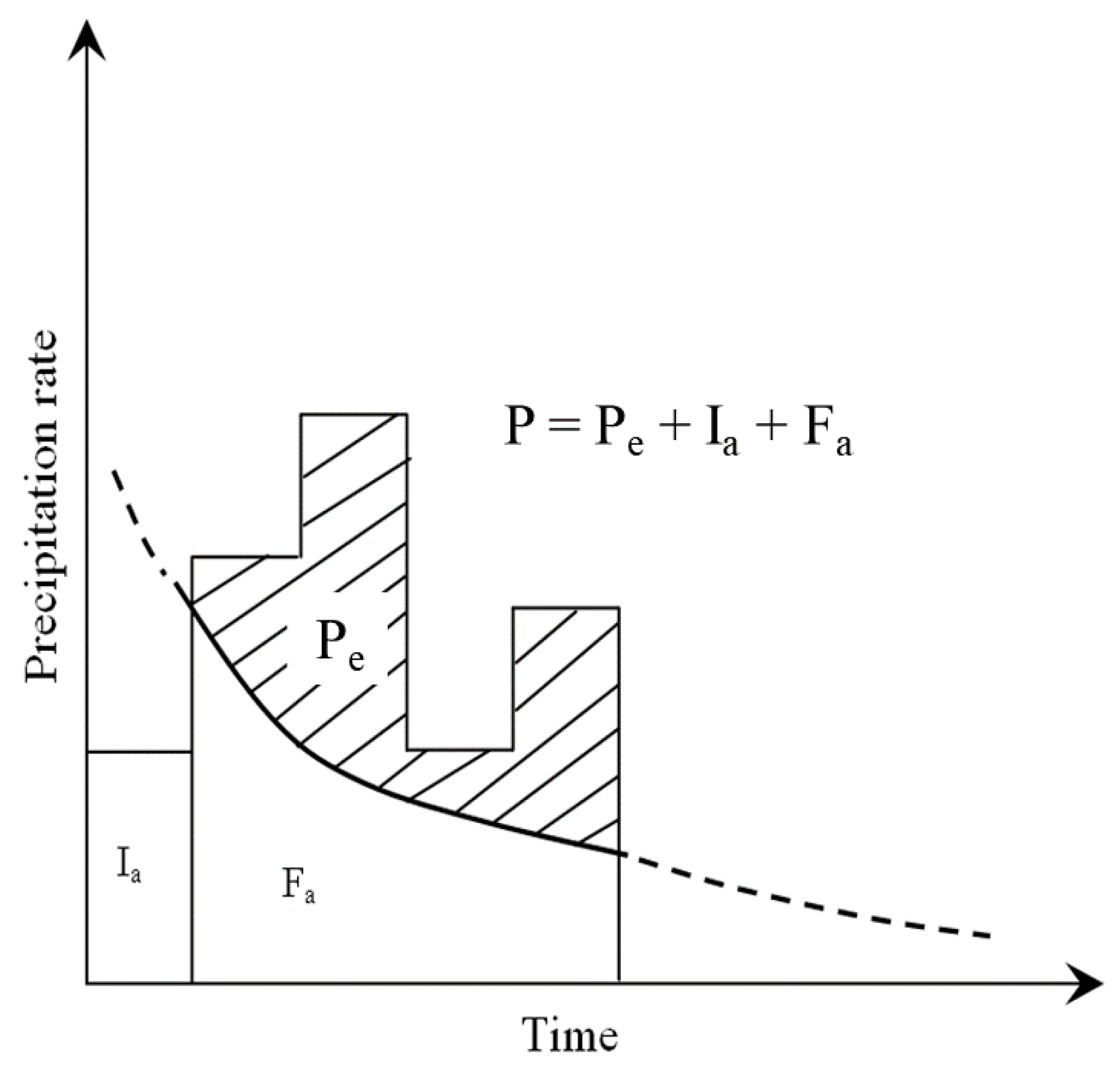
In the GLEAMS modeling approach, the abstraction is modeled continuously, and it is related to soil information which is not available for the study area. Thus, this formula was modified with the assumption that the total storm runoff infiltration minus the initial abstraction (the numerator in the exponential function) is equal to the continuing abstraction (Fa) (see Figure 2).
In doing so, Equation (20) becomes
C = C 1 e x p [ ( P P e I a ) ( K d ) ( 1 P O R 2.65 ) + P O R ] ,
where P is the total rainfall, Pe is the rainfall excess, Ia is the initial abstraction, and Fa is the continuing abstraction.
The final dissolved concentration was calculated based on the GLEAMS approach [40], which is also applied in the ANSWERS model [44].
C d k t = C β 1 + k β ,
where C and Cdkt are indicated in Equations (20) and (18), respectively, β is an extraction coefficient, and k is the partition coefficient.
{ β = 0.5 ,                            k 1 β = 0.598 e 0.179 k ,     1 < k 10 β = 0.1 ,                            k > 10
Nitrogen nitrate (N-NO3) is not attached to the soil particles, and it is always in solution (e.g., in overland flow, infiltrating, percolating water). For nitrate, the partitioning coefficient was set to zero as nitrate exists only in the dissolved phase, and the extraction coefficient was set to 0.5. For nitrogen ammonium (N-NH4) and phosphorus phosphate (P-PO4), the partitioning coefficient was larger than 10 and, thus, the extraction coefficient was set to 0.1 [44].

2.4. River Routing and Point Sources

The transport of nutrient and sediment through a stream/river is routed in the flow routing module. In addition, this module should take into account the contribution of point sources (i.e., wastewater discharged from industrial areas). The river routing component was adopted from the diffuse–pollution–load (D-POL) model [46]. The model was applied to simulate dissolved nutrients in small Mediterranean catchments during flood events. The D-POL model is an integrated system including catchment pollutant loads driven by the rainfall and river routing. The D-POL model is based on a rainfall-load semi-distributed approach, and it was successfully calibrated against a 20-flood dataset, validated against a 10-flood dataset, and applied to many flash flood events. However, only the river routing was adopted since other model components of D-POL do not include particulate pollutants caused by erosion/sedimentation processes. The most important assumption in this river routing is the pollutant concentration to be conserved along the river reaches during storm events.
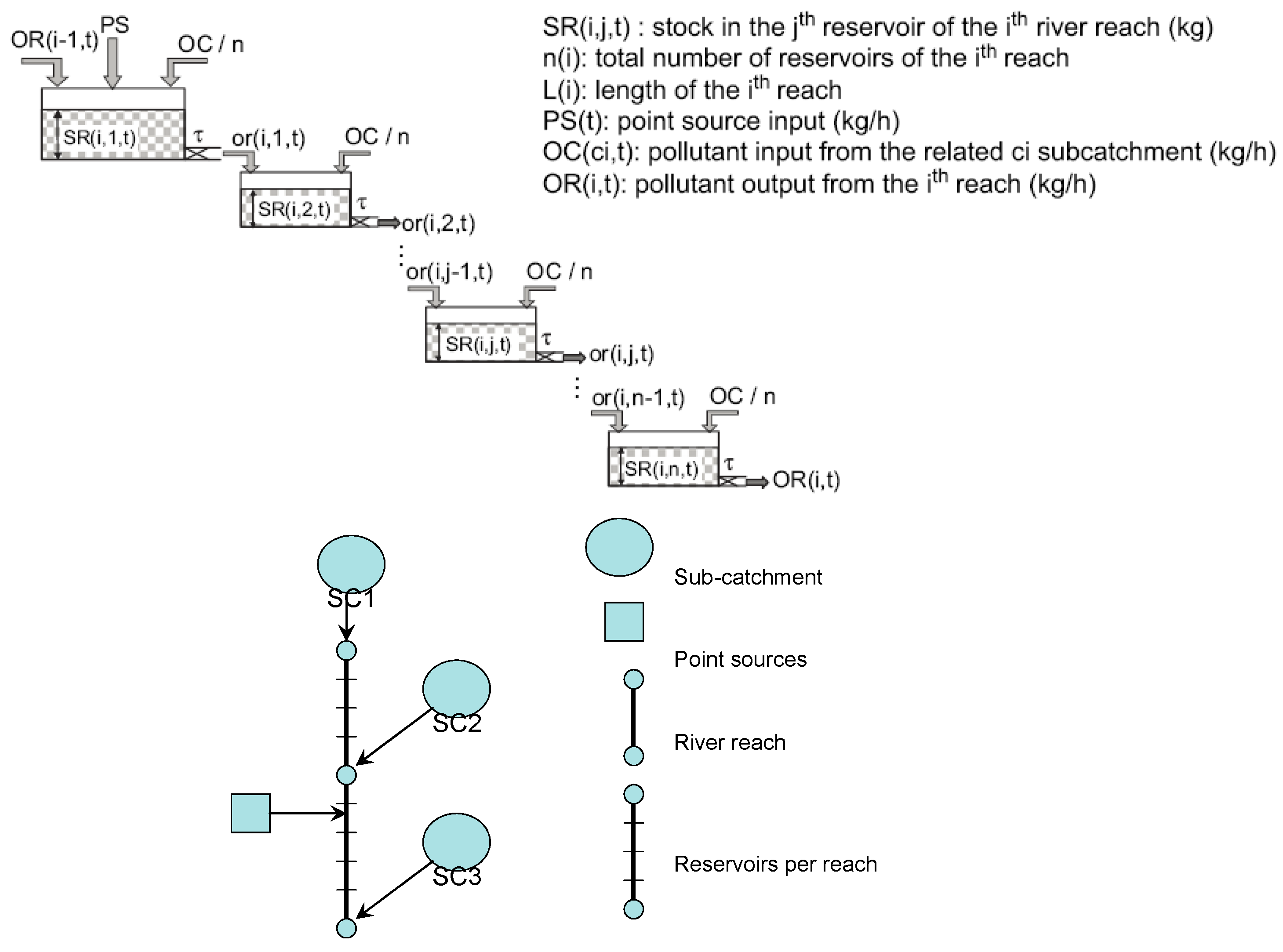
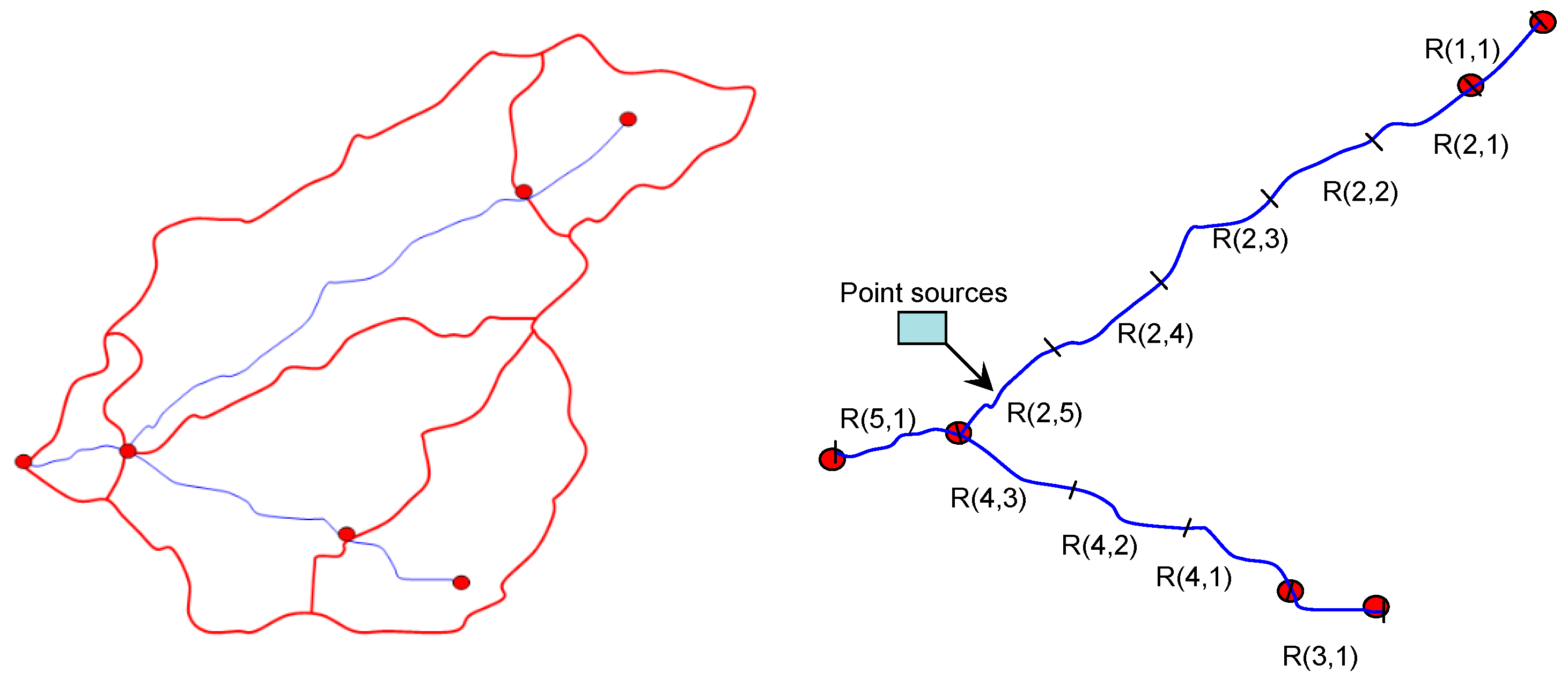
The river is discretized into reaches and each reach is discretized into a number of reservoirs depending on the length of each reach. Figure 3 (top) shows how pollutant sources, sinks, and changes of storages are conceptualized within the reach, while Figure 3 (bottom) shows how the reaches are connected within a catchment.
Equations for every reach and reservoir are based on the mass conservation law, where the change of a storage is equal to the differences between the output and input, presented as follows:
The changes of storage at the ith reach and first reservoir at time t,
d S R ( i , 1 , t ) d t = P S ( i , 1 , t ) + O C ( c i , t ) n ( i ) + O R ( i 1 , t ) o r ( i , 1 , t ) .
The changes of storage at the ith reach and jth reservoir at time t (1 < j < n(i)),
d S R ( i , j , t ) d t = P S ( i , j , t ) + O C ( c i , t ) n ( i ) + o r ( i , j 1 , t ) o r ( i , j , t ) .
The changes of storage at the ith reach and nth reservoir (last reservoir of reach i) at time t,
d S R ( i , n , t ) d t = P S ( i , n , t ) + O C ( c i , t ) n ( i ) + o r ( i , n 1 , t ) O R ( i , t ) ,
o r ( i , j , t ) = 1 τ S R ( i , j , t ) ( 1 j n ( i ) ) ,
T = 1 τ ,
n ( i ) = L ( i ) L b ,
where SR(i, j, t) is the stock of pollutants in the jth reservoir of the ith reach (kg), n(i) is the total number of reservoirs of the ith reach, L(i) is the length of the ith reach, PS(i, j, t) is the point sources input (kg/h) to the jth reservoir of the ith reach, OC(ci, t) is the pollutant input from the related sub-catchment ci (kg/h), OR(i, t)/or(i, t) is the pollutant output from the ith reach (kg/h), τ is the lag-time of the river reservoirs (h) (to be fitted by calibration), Lb is the basic length (e.g., 1000 m), and T is the transport parameter (L/h).

2.5. Model Uncertainty

The Monte Carlo simulation method was utilized for an uncertainty analysis. The Monte Carlo simulation technique involves random sampling of model input and/or model parameters to produce hundreds or thousands of scenarios (i.e., outputs; see Reference [47]). The model results are stored and then evaluated statistically. In this manner, an uncertainty in model input and/or model parameters, presented as probability distributions, will propagate through simulation systems. In this study, the Monte Carlo simulation was combined with the Latin hypercube sampling method [47]. Every simulation was run for 1000 time steps within a Microsoft Excel file. The software was assisted by an add-in program called RiskAMP Monte Carlo Add-in for Excel® (https://www.riskamp.com). For each parameter and input, the uniform distribution was applied.
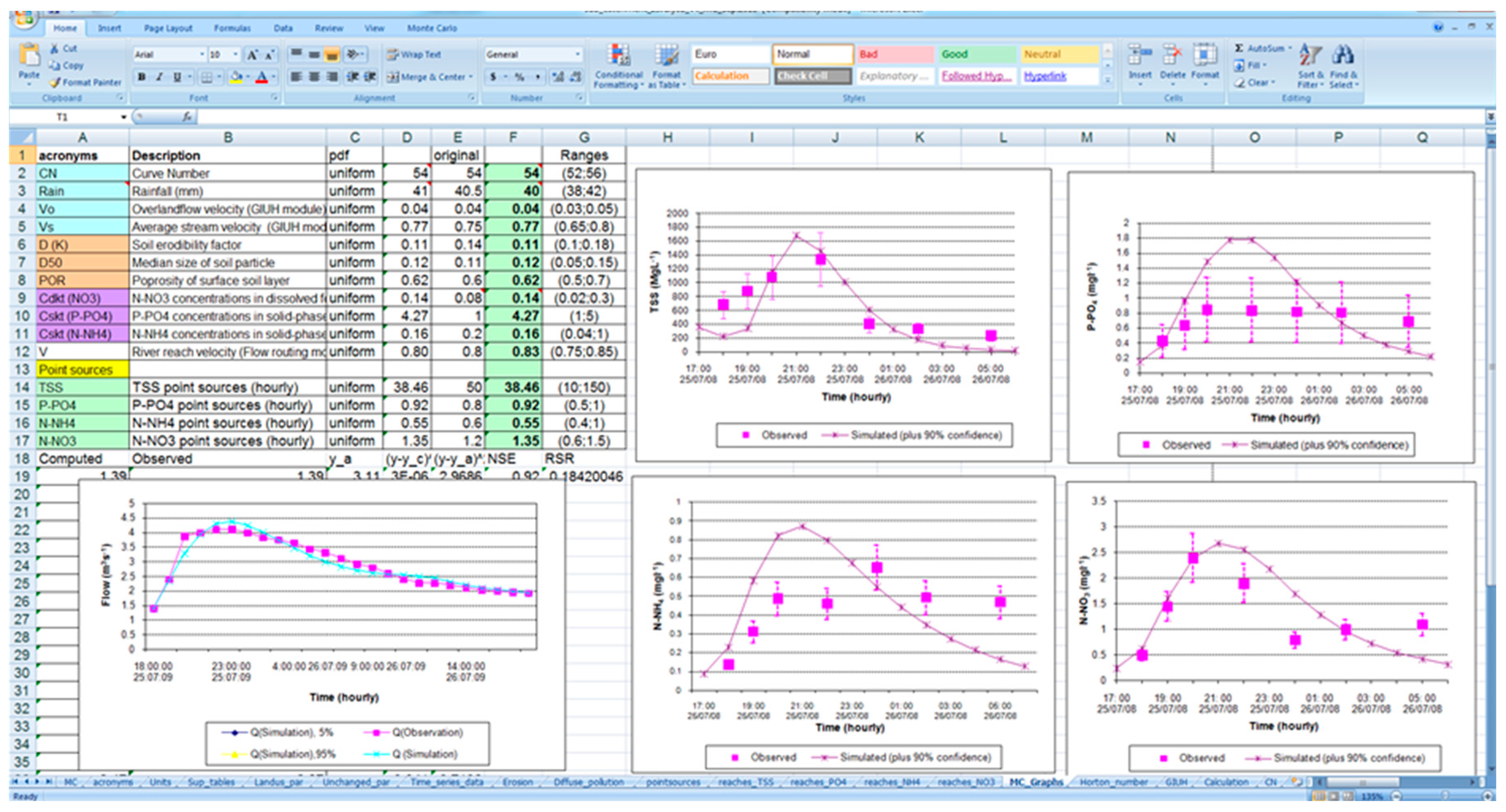
A full water quality model including all modules merged in a spreadsheet is shown in Figure 4.

3. Application

3.1. Study Area

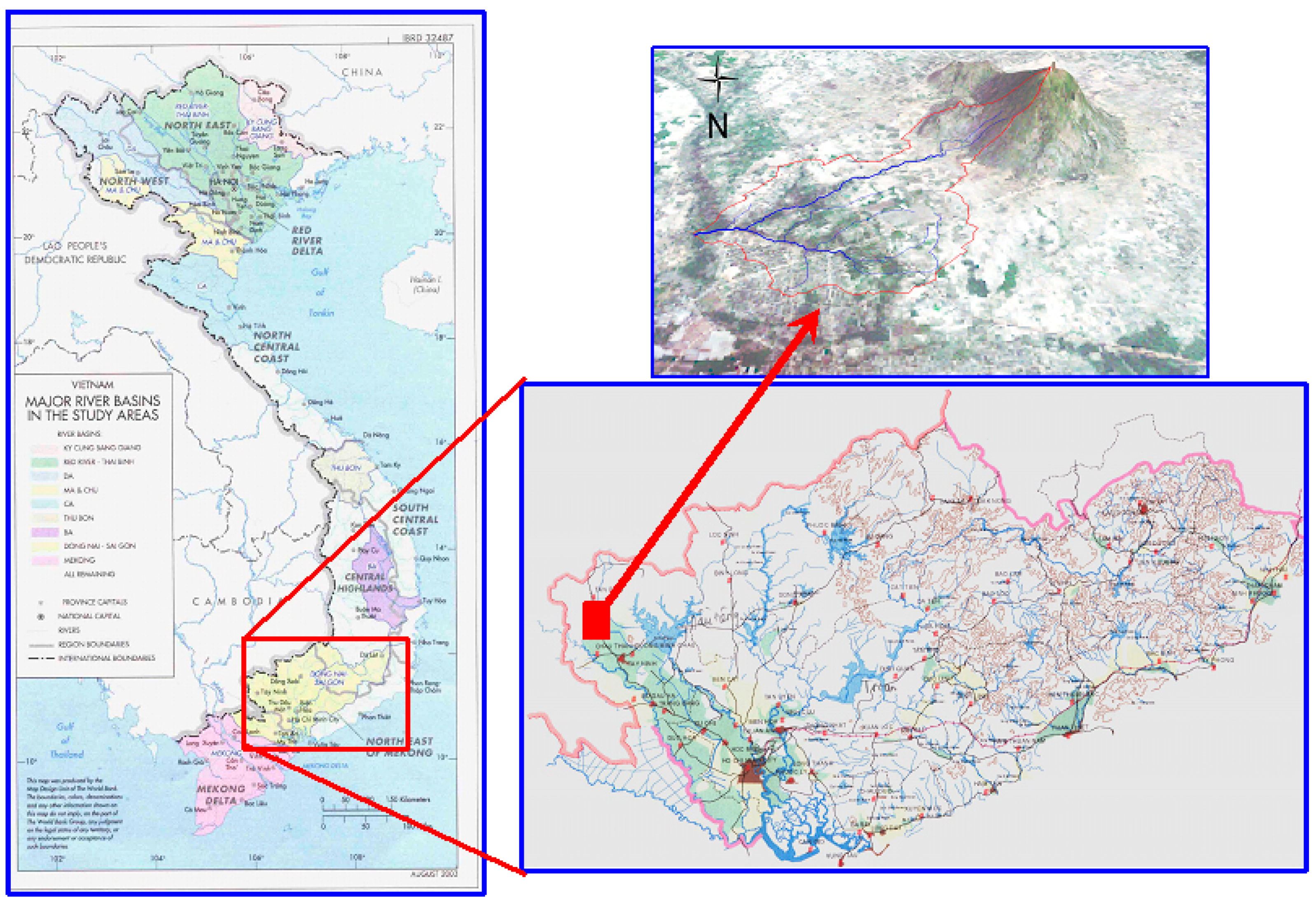
The study area was the Tra Phi catchment located within the Dong Nai river basin (Figure 5); this study area was considered as a pilot area because it has the typical hydrologic condition of Dong Nai river basin, a combination of various land uses, and industrial areas containing point sources. The Dong Nai river basin is the largest national river basin in southern Vietnam, and it is considered as a hot spot of water pollution in Vietnam [48] (p. 78).
The study area is affected by the tropical monsoon climate; therefore, it has two distinguished seasons: the dry season (from December to April) and the rainy season (from May to November). Extreme rainfall events up to 180 mm/h often occur in the area during the rainy season [49]. The catchment is characterized by a heterogeneous topography ranging from 2–30 m above sea level (a.s.l.) in low-land areas to about 1000 m a.s.l. at the water head. The catchment area is about 21 km2, including agriculture (66%), forest (11%), wetland (3%), semi-urban areas (13%), and urban areas (7%). Gray soil (Acrisol) is major soil type in the catchment [49]. The only identified point source of wastewater comes from a factory which produces tapioca starch from cassava (tapioca) roots. The company produces on average 30 tons of tapioca starch per day, which generates about 360–600 m3 of wastewater per day [50]. An analysis of the water quality data of the main Tay Ninh river can be found in Nguyen and Meon [3].

3.2. Model Set-Up

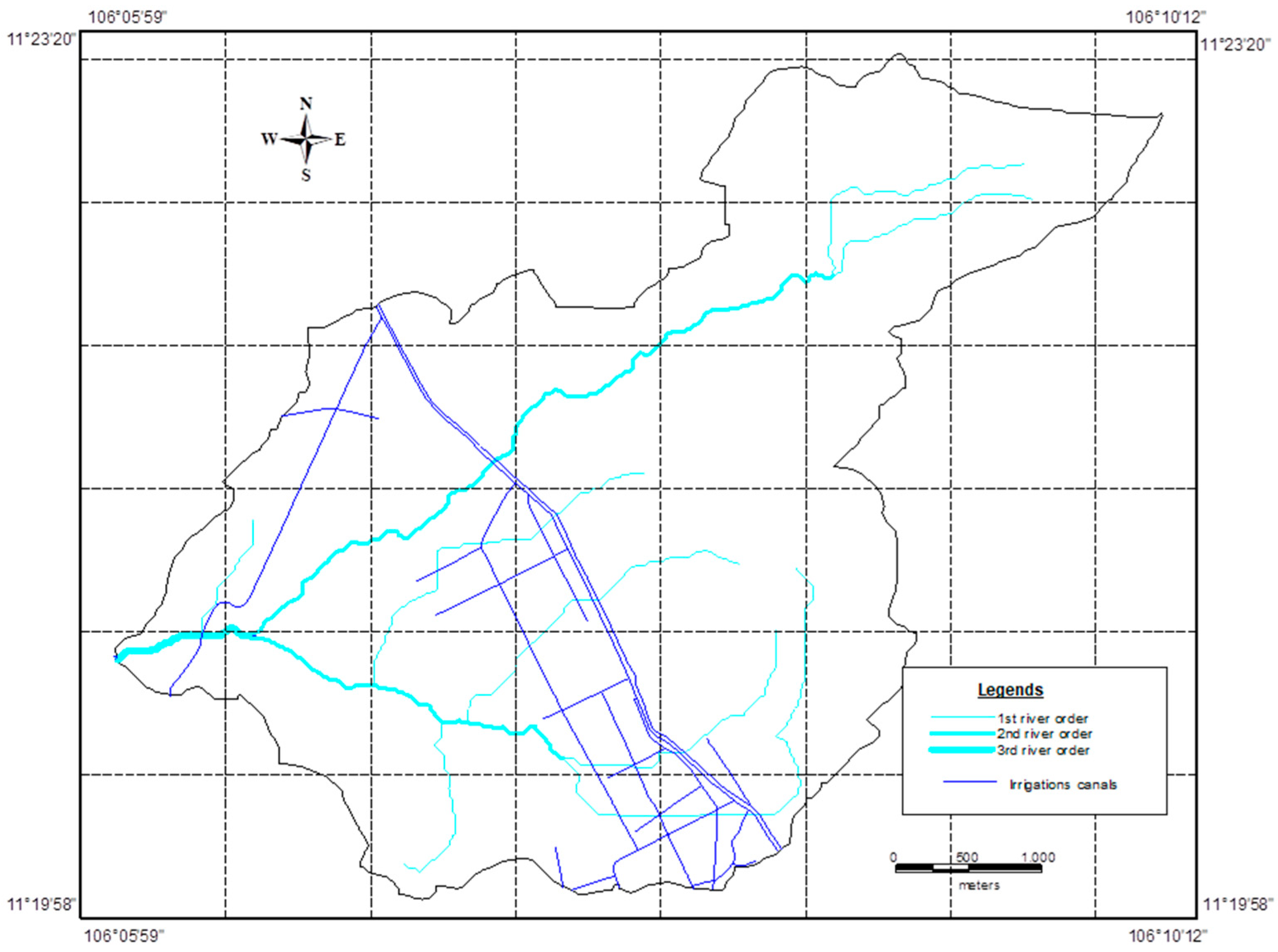
The Tra Phi catchment is a third-order catchment with a drainage density of about 1250 m/km2. There is an irrigation canal system through the catchment transferring water from Dau Tieng reservoir for irrigation purposes (Figure 6). This system is independent of the river network in terms of direct contribution to river flows. In this study, it was assumed that the contribution of irrigated water to the river network was negligible.

3.3. Calculation of Model Parametes

3.3.1. Hydrologic Calculations

Model parameters of the GIUH include the Horton’s ratios, hillslope, and stream flow velocity.
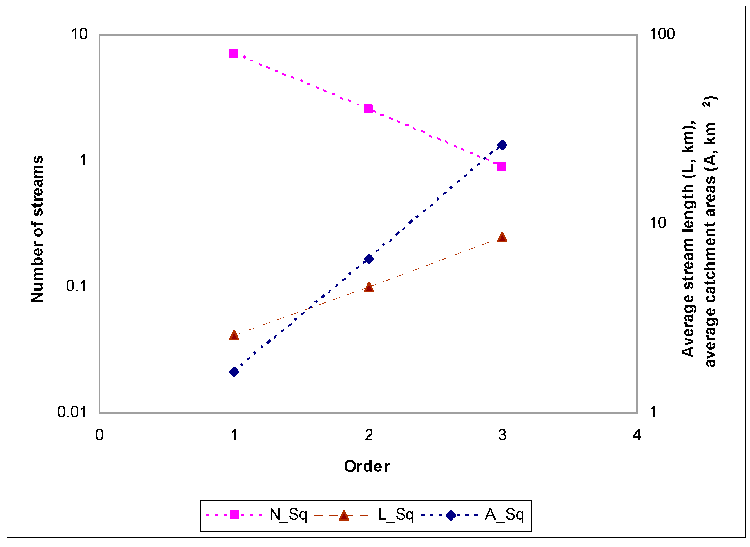
Horton’s statistics including RA, RL, and RB parameters were calculated using a new functionality in ILWIS called “Horton statistics” in module “statistical parameter extraction” (in “DEM—Hydro-processing”) [51]. The procedure included three calculation processes as follows: (i) calculating the number of streams, the average stream length (km), and the average area of catchments (km2) for all streams (represented by C1_N, C1_L, and C1_A in Figure 7); (ii) calculating the expected values of the number of streams, the average stream length (km), and the average area of catchments (km2) by means of a least-squares fit (represented by C1_N_LSq, C1_L_LSq, and C1_A_LSq in C1_N_LSq, C1_L_LSq, and C1_A_LSq in Table 1); (iii) calculating the area ratio (RA), length ratio (RL), and bifurcation ratio (RB) from the slopes of each fitted line connecting the expected values shown in Figure 7 (results shown in Table 1).
The obtained values and the least-squares fit were visualized using a Horton plot to inspect the regularity of the extracted stream network and to serve as a quality control indicator for the entire stream network extraction process. It is expected that the number of streams shows a decrease for subsequent higher-order Strahler numbers and longer streams, and that the catchment areas show an increase for subsequent higher-order Strahler numbers [52].
From the Horton plot (Figure 7) and Table 1, it can be assessed that the drainage network is well extracted, and that the Horton numbers are representative and fall within the expected range; thus, they could be used without any calibration. The extracted river network is presented in Figure 6.
The above section “GIUH development” showed how to derive the GIUH, whereas the calculation of the surface discharge for each event is described below.
The effective (excess) rainfall was computed according to the Soil Conservation Service (SCS) runoff method (see Reference [29] for the original, and Reference [30] (p. 147) for the latest one). To calculate the curve number (CN) value, the land-use and soil maps used were based on the SCS table. The CN values of each map unit were aggregated for the whole catchment by means of GIS to get an average CN value (e.g., see Reference [53]). Then, the effective rainfall was calculated by the SCS curve number method.
P e =   { ( P 0.2 S ) 2 P + 0.8 S         i f         P > 0.2   S 0                           i f         P < 0.2   S ,
where Pe is the effective rainfall or direct runoff expressed as a depth (mm), P is the total observed rainfall (mm), and S is the potential maximum retention (mm), calculated as
S = 25,400 C N 254 .
After having the effective rainfall, Horton’s statistics values were used to derive the GIUH, the surface runoff was calculated (see Reference [30] (p. 211)), and the discharge was determined by taking into account the catchment area. The catchment flow was composed of three components: (1) surface flow (overland flow), (2) subsurface runoff or interflow, and (3) base flow or groundwater flow. In the GIUH approach, the model can basically simulate the overland flow plus parts of the interflow which leave the unsaturated zone and arrive as surface flow at the river. Therefore, from the observed hydrograph, the contribution of base flow needs to be subtracted. In this study, the base flow was separated manually using the constant slope method [54].
The CN value, overland flow velocity (Vo), and the stream velocity (Vs) need to be calibrated against the observed discharges. Final values obtained from the calibration are shown in Table 10.

3.3.2. Erosion and Sediment Calculation

The development of the erosion/sediment yield module includes four main steps: (1) extracting runoff values from hydrologic calculation; (2) calculating soil detachment by runoff and soil detachment by rainfall; (3) calculating sediment transport capacity; and (4) calculating sediment yield. According to Section 2.3, several model parameters related to soil, catchment characteristics, rainfall, and runoff are needed. In particular, these are (1) soil data: median size of soil particle (D50), specific weight of sediment (σ), and soil erodibility factor (D); (2) land-use data: ground cover factor (GC) and canopy factor (CF); and (3) physical characteristics of catchment: slope (So), catchment areas, and overland flow length (L).
Model parameters included constants and calculated or estimated parameters. The first ones were adopted from literature, as shown in Table 2, while the latter ones were calculated for each land use and soil type within a catchment, and then aggregated for each sub-catchment. The catchment parameters were calculated based on GIS/DEM processing, and they were assigned for each sub-catchment (Table 3). Since the catchment was mostly distributed by gray soil (Acrisol), the soil parameters were kept as unique values while other parameters were aggregated according to different land-use types (Table 4). The predicted sediment in the model, therefore, should be clay. In this approach, the clay fraction (Fcl) in sediment calculated based on the approach presented in Hartley [31] was adapted as follows:
F c l = 0.26 O c l ,
where Fcl is the clay fraction in detached sediment, and Ocl is the clay fraction in matrix soil (0.04 for Acrisol).

3.3.3. Nutrient Loading Calculation

Data requirements for the nutrient loading model are rather simple. Hourly input data for the nutrient loading component (i.e., runoff (Qkt) and soil loss (Xkt)) were obtained from the hydrology and erosion modules. Other parameters, such as soil porosity and solid-phased concentration, were estimated from the literature or soil sampling. Model outputs were constituent loadings (hourly) at each outlet of the sub-catchments which were later used as inputs for the flow routing module.
The nutrient parameters were calculated for each land-use type, and they were aggregated for each sub-catchment; the results are shown in Table 5. Since the entire catchment was mostly distributed by gray soil (Acrisol), the soil porosity of 0.6 obtained from the field survey was applied for the whole catchment. The overland flow length was similar to that applied in the erosion/sedimentation module.
The calibrated values of Cdkt and Cskt were smaller than their values observed by experiment (e.g., in Reference [17]). The reason could be due to the retention effects within the catchment, as well as because of the aggregation technique in GIS processing.

3.3.4. River Routing Calculation

The Tra Phi catchment is discretized into five sub-catchments corresponding to five reaches. In general, discretization is oriented to the hydrological similarity (soil, topology) within a sub-catchment. In addition, each reach is discretized into a number of virtual reservoirs depending on their lengths (e.g., about 1000 m for each reservoir; Figure 8 and Table 6)
The module simulates flood events on an hourly time step. Data input for this flow routing included diffuse sources, as well as the point source, reach length, average velocity, and initial conditions. The diffuse sources obtained from the sediment and nutrient module were sediment and nutrient loadings from the sub-catchment. The point source was wastewater loading from the identified company at a specified location for each simulated constituent (in Figure 8, it is located at Reach 2, Reservoir 5).
Constituent loadings can be read at every reservoir, along with the reach (as output). Concentrations can only be produced at catchment outlets where the flow discharge is available for converting the loading to concentration. Information on the Tra Phi river reaches can be obtained by GIS processing, and the data are shown in Table 6 and Table 7.

4. Results and Discussions

4.1. Sensitivity Analysis

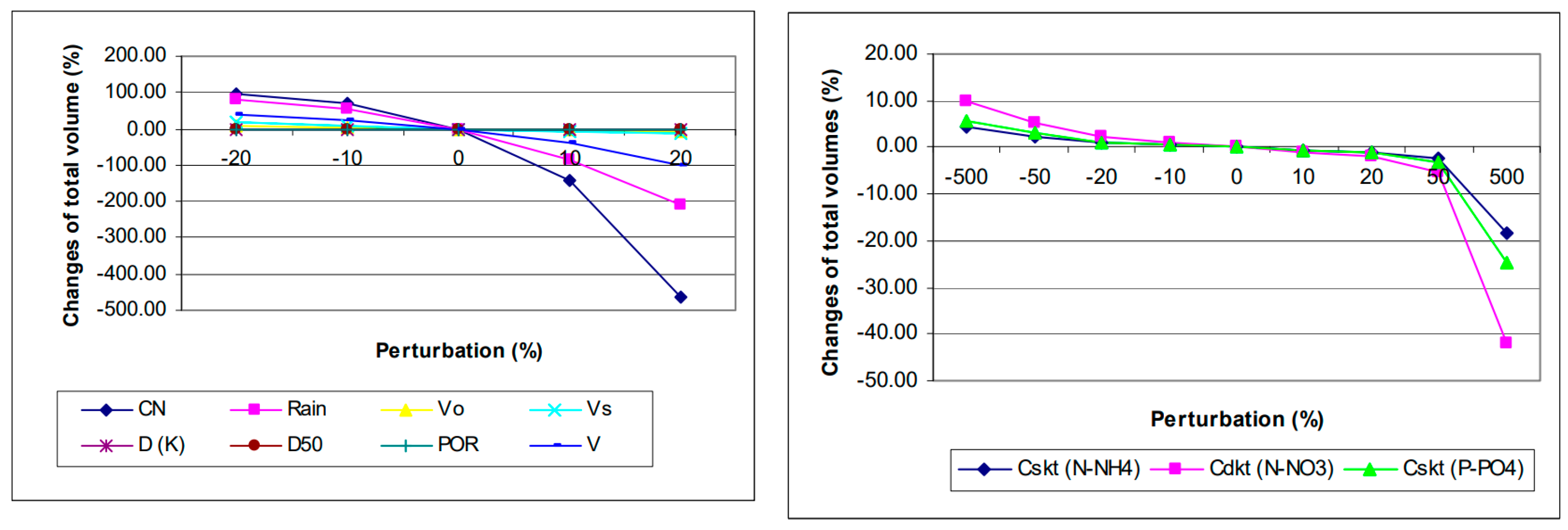
Model parameters were analyzed for the four main modules (i.e., hydrology, erosion, nutrient loading, and river routing). Table 8 shows the parameters and their variations applied in this analysis. The sensitivity was calculated based on perturbing the model parameters within the permitted physical ranges or observed extreme ranges, and observing the variation of model results (e.g., total flow discharge or total loadings for the whole event). An example resulting from the sensitivity analysis for nutrients is shown in Figure 9. It can be summarized in four points. Firstly, within the hydrological components, the CN value and the rainfall input are the most sensitive factors to model results. The CN value is more sensitive than the rainfall input to the variation of flow discharge volume. The velocity parameters (Vo, Vs) do not influence the total volume, but highly influence the shape of hydrograph as the velocity parameters are used to calculate the travel time of the rain drop in the catchment. Secondly, the velocity parameters V from the river routing module and (Vo, Vs) from hydrological module are the next most sensitive parameters. The effects from the velocity on the shape of hydrograph will significantly contribute to total loadings, since the loading is a function of flow discharge and concentration. Thirdly, the effects of soil parameters K, D50, and POR on the final results of sediment and nutrient loadings are very small in comparison to hydrological parameters, because the sediment and nutrient loads are strongly driven by hydrological processes (e.g., rainfall and runoff) in flood events. In addition, the nutrient loading parameters (i.e., Cdkt (N-NO3), Cskt (P-PO4, N-NH4)) can only show clear variations when increasing up to 500% (Figure 9). Fourthly, the changes of point sources also significantly affect the model results as they contain a large amount of pollution loaded directly into the rivers. The variation is about 35% when the perturbation is less than 50%. However, once increasing the perturbation to five times (500%), the variation is about 280%. This aspect is essential once dealing with illegal wastewater dumped directly from factories into the rivers as mentioned in Section 1.

4.2. Model Results

Model results of an event from 25–27 July 2008 (for calibration) are described in this section. The results of another event from 14–15 August 2008 (for validation) are presented in the Appendix.
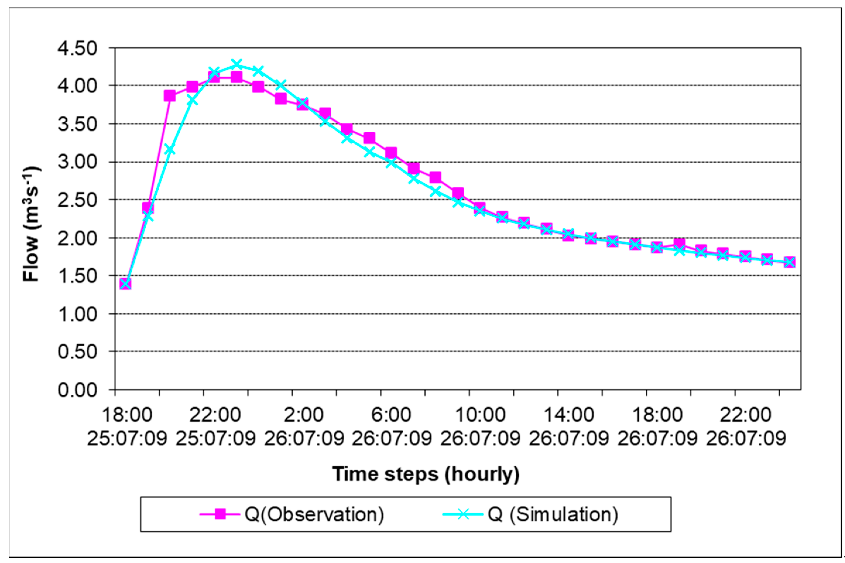
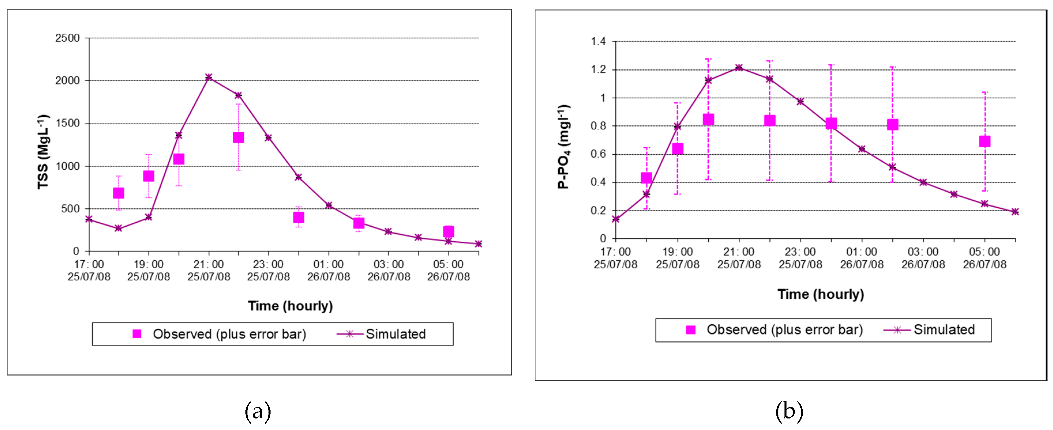
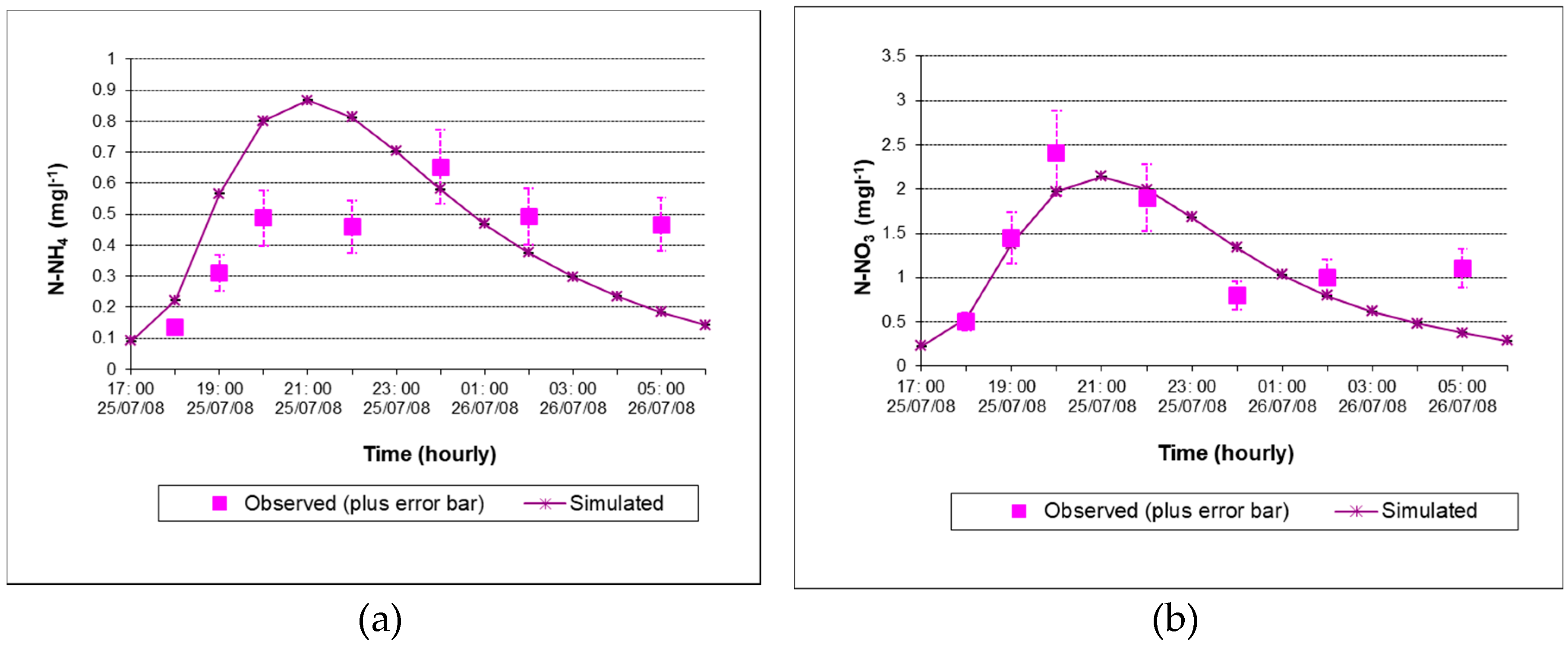
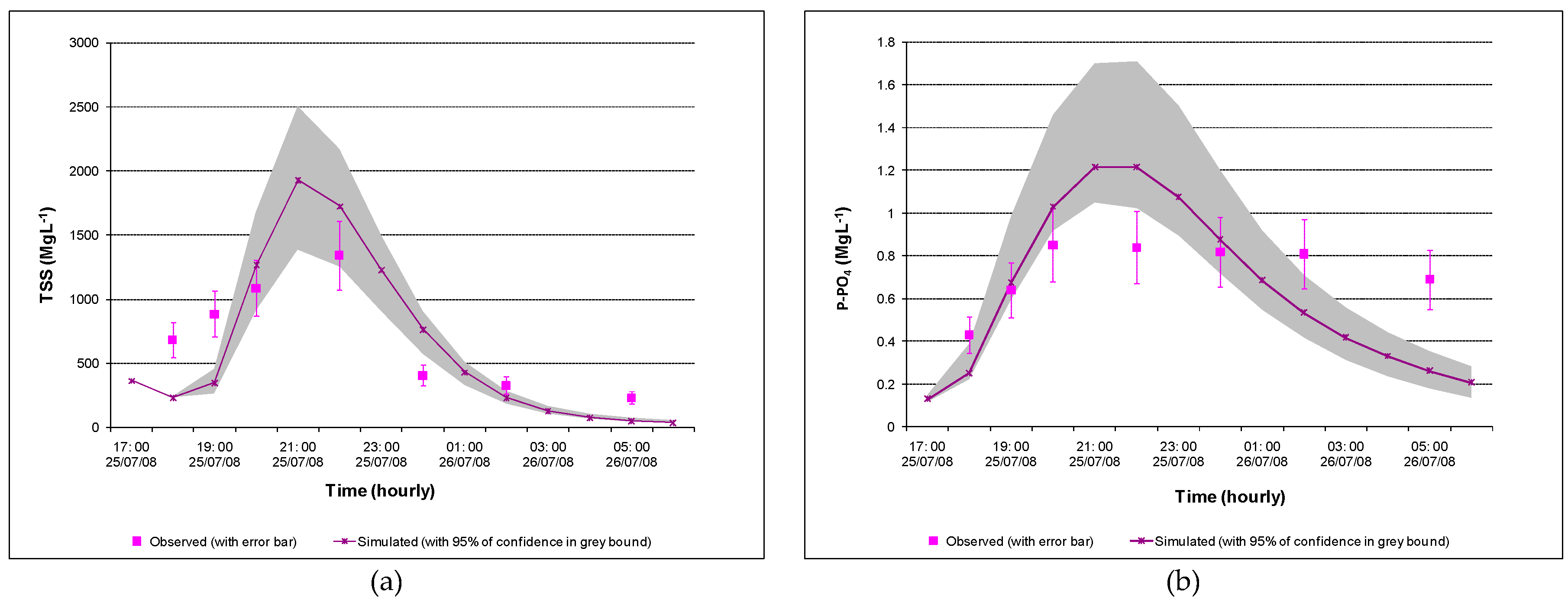
The hydrological parameters and inputs (e.g., CN, rainfall) significantly affect the results of other model components (TSS and nutrients). Therefore, these parameters need to be carefully calibrated before considering other parameters. Table 9 shows the evaluated parameters for flow, total suspended solid (TSS), phosphate (P-PO4), ammonium (N-NH4), and nitrate nitrogen (N-NO3), which are also illustrated in Figure 10, Figure 11, Figure 12 and Figure 13. The model results are plotted together with observed data whose error bars were calculated using Harmel’s method [55]. The cumulative measured data errors due to sampling, preservation, and analysis of total suspended solid, nitrogen ammonium, nitrogen nitrate, and phosphorus phosphate were 28%, 18%, 18%, and 50%, respectively. The results can be summarized in five points. Firstly, the runoff flow discharge is well simulated, including the curve, peak, and time to peak. Furthermore, based on the model evaluation statistics [56], the runoff flow simulation is in very good agreement with the observation due to its Nash–Sutcliffe efficient (NSE), index of agreement (d), coefficient of determination (R2), and percent bias (PBIAS) being 0.9, 0.97, 0.90, and 0.26, respectively. Secondly, regarding water quality parameters, based on the PBIAS values (see Table 4 of [57]), the parameters of P-PO4, N-NH4, and N-NO3 are very good (PBIAS < ±25). Only TSS (PBIAS = 29.97) is a bit worse than other parameters in the comparison between simulation and observation; however, this value is still in the good rating range (±25 < PBIAS < ±40). Furthermore, the d index shows a good agreement between simulated and observed results for runoff flow discharge, TSS, and nutrients. Thirdly, prediction of N-NH4 and N-NO3 is better than prediction of P-PO4. The reason may be that the nitrogen parameters are mainly related to the runoff processes, while P-PO4 is dependent on the erosion process adding into the runoff processes. In addition, as shown above, the possible errors of P-PO4 are also very high (50%), as they can accumulate errors, leading to a worse performance of this parameter. Fourthly, the model should be further improved by implementing more certain monitoring techniques, and a higher frequency of measurement. Fifthly, the model did not adequately capture the receding curve. The reason could be the retention effects of agricultural fields, especially rice fields, which were controlled by farmers (e.g., releasing water after rainfall events to ensure that the field is not too inundated). In addition, the omission of nutrient and sedimentation transformation processes in the river routing is another factor that may lead to model underestimation.
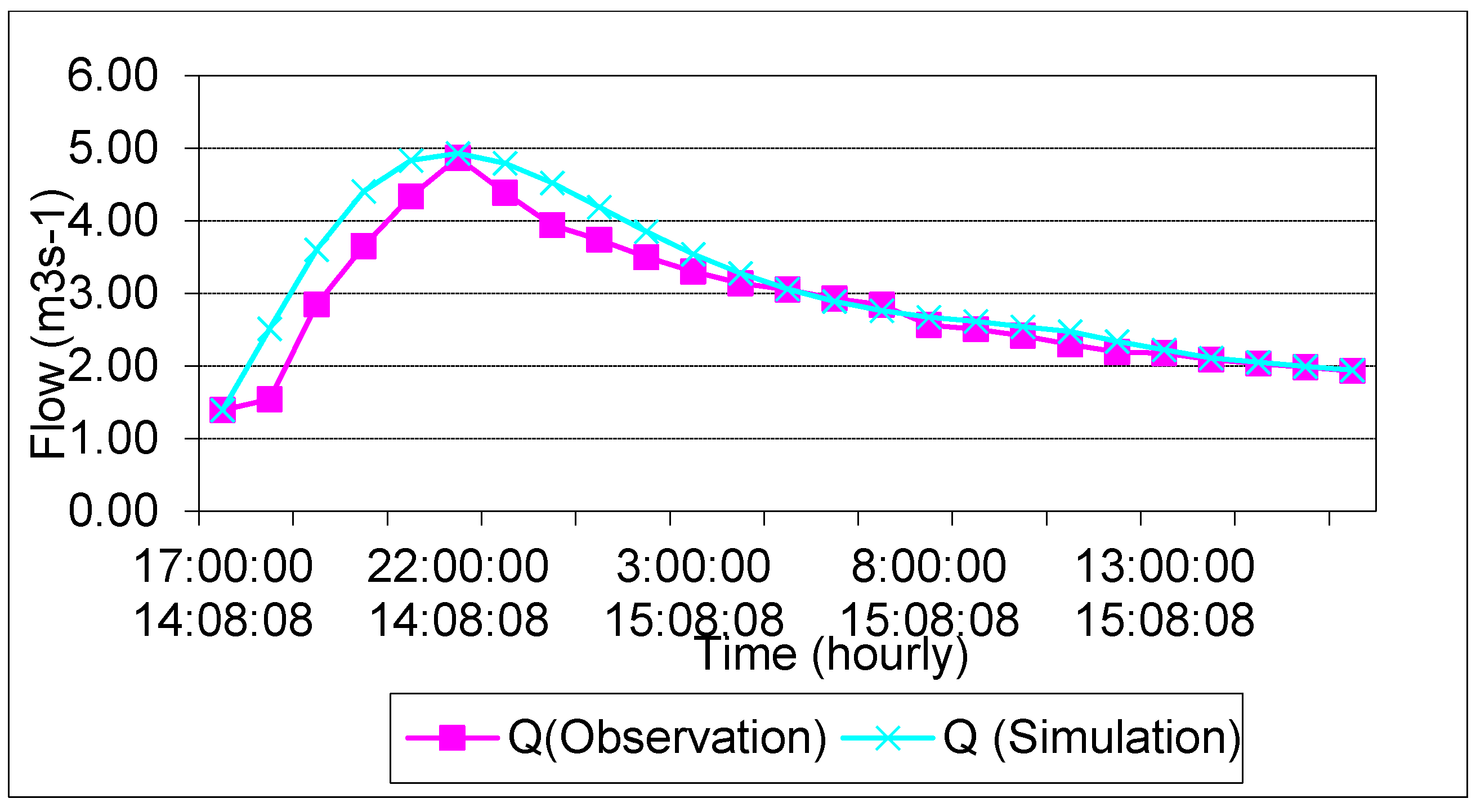
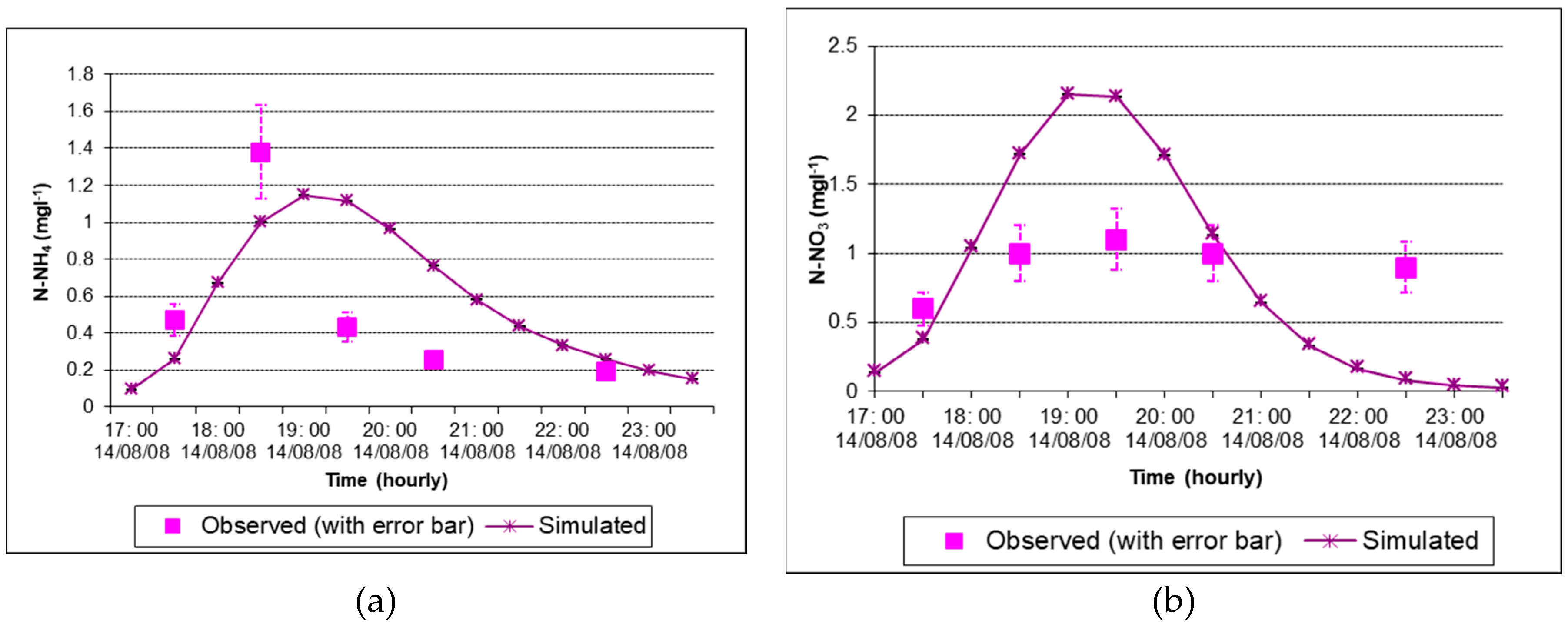
Similar trends are obtained for the validated event from 14–15 August 2008, as shown in Table A5 and Figure A1, Figure A2 and Figure A3 in the Appendix.

4.3. Model Uncertainty Analysis

Every simulation was run for 1000 time steps within a Microsoft Excel file. The software was assisted by an add-in program called RiskAMP (RiskAMP Monte Carlo Add-in for Excel®). For each parameter and input, uniform distribution was applied. Data for the Monte Carlo simulations are shown in Table 10.
The sensitivity analysis showed that the CN, flow velocity (river routing) parameters, and rainfall (input) are the most sensitive factors for the model results. Thus, firstly, these three parameters and the input were calibrated so that the Nash–Sutcliffe efficiency (NSE) ranges within 0.85–0.95 were considered as acceptable (e.g., as in [58]). Since then, different scenarios were developed in order to see how these parameters propagate to model results. Results are shown in Table 11 and Figure 13 (for TSS and P-PO4).
Due to the high effects of the CN parameter, rainfall, and flow velocity, the propagation of other parameters is not clearly seen (Table 11). The uncertainty boundary is greatly reduced if these parameters are excluded in the uncertainty analysis. The results are also consistent with those obtained from the sensitivity analysis.
The uncertain boundary is rather large, especially during the peak flows, whereby, upon comparing to the mean values, it can be more than 100%. However, the simulation results show that, when including the boundary (confidence interval of 90%) in Monte Carlo simulations, a very good agreement between model simulation and observation data is obtained.
The variation in model output is also highly affected by the change of point sources, especially when extreme disposal occurs. This was also shown in the sensitivity analysis, where a fivefold increase of point source compared to normal can change the results up to 280%.

5. Conclusions

In this study, a water quality model was developed to simulate nutrient dynamics for sparsely gauged catchments during flood events. Most of the model input data were deduced from various methods, which were applied for data-scarce regions. The hydrological component was based on the GIUH [21], using parameters obtained from GIS processing, which was verified and applied for several flood events in Vietnam [20]. The erosion/sediment component was based on Hartley’s approach [31], which was verified by Hartley [32] and Leon et al. [59]. In the nutrient loading component, the loading function method was applied, whereby the nutrient loads could be integrated from the outputs of hydrological and erosion processes. The loading function method was successfully applied by Haith and Tubbs [37] and Haith et al. [38,39]. The river routing component was adapted from the D-POL model [46], in which the river was simply discretized into reaches, followed by each reach being discretized into reservoirs; the pollutant was integrated over nutrient loads and sediments obtained from the nutrient loading component, and loadings from point sources were also added into this component. The simplified model structure and limited model parameters are the most appealing features of the model. All model components are coupled and controlled within one Excel Spreadsheet Macro. The running environment is within an Excel Spreadsheet Macro, and this feature makes the model user-friendly and robust, with easy installation. Furthermore, an add-in Monte Carlo simulation tool was implemented in this modeling system to provide a reasonable uncertainty analysis tool for the users to calibrate the input parameters and to validate model results. Implementations of different model components can be easily accessed and monitored under Excel Spreadsheet functions. This aspect is especially useful when implementing the sensitivity and uncertainty analysis. The coupled system can represent the system dynamics, such as flow discharge, suspended solid, and nutrients during flood events. In addition, the point source disposal is also included. In addition, because of the capacity of the model in utilizing GIS and remote sensing data, many model parameters can easily be extracted. This characteristic is very important when dealing with data-scarce regions (ungauged catchments). Therefore, the application of the model confirmed the necessity to adapt the model complexity to the data availability of the investigated area. The success of the developed model proved the importance of selecting suitable model structures for specific regions and applications. There are various available models such as SWAT and HSPF; however, they require intensive input data and, consequently, it is hard to deal with sparsely gauged and ungauged catchments. Our approach was based on findings of previous studies (e.g., [60,61]), whereby all the dominant processes in the system should be captured in the model, whereas processes of minor importance should be neglected or treated in a less complex manner.
Based on the uncertainty simulation results, possible scenarios can be explored when dealing with many uncertain sources (a similar conclusion was drawn in [62]). A further study should focus on reducing the uncertainty caused by input data (e.g., obtaining more reliable data by improving monitoring data in time and space). For example, a high impact on model results was also found in rainfall data. Given only one observation station in the catchment covering an area of extreme topographic variation, the uncertainty propagation due to incorrect rainfall data is a critical issue. Therefore, improving rainfall observation is highly recommended.

Author Contributions

Investigation, H.Q.N.; methodology, H.Q.N., G.M., and V.T.N.; software, H.Q.N.; supervision, G.M. and V.T.N.; writing—review and editing, V.T.N.

Funding

This research was initially funded by the German BMBF and the Vietnamese Ministry of Science and Technology under grant number 02WA0991; and finally funded by Institute for Computational Science and Technology (ICST) under grant number 31/2017/HD-KHCNTT.

Acknowledgments

This research was initially funded by the German BMBF and the Vietnamese Ministry of Science and Technology under the grant number 02WA0991; and finally funded by Institute for Computational Science and Technology (ICST) at Ho Chi Minh City, Vietnam under the grant number 31/2017/HD-KHCNTT. Eventually, the authors would like to thank the anonymous reviewers for their valuable and constructive comments to improve our manuscript.

Conflicts of Interest

The authors declare no conflicts of interest.

Appendix A

Table A1. Land-class schemes [59].
Class NoClass TypeTypical Land CodeGCCF
Class 6ImperviousUrRe0.10.9
Bare groundUrGd0.10.9
ForestsNUWod0.80.4
Crops LowVegNUSg0.50.6
WetlandsNUWe0.60.5
WaterNUWa00
Class 10ImperviousUrRe0.10.9
Bare ground lightNUFf0.10.9
Bare ground darkUrTs0.20.85
Forests lightNUWol0.80.35
Forests denseNUWod0.90.3
GrassNUGr0.50.6
Crops lowNUSg0.60.5
Crops highNURc0.70.4
WetlandsNUWe0.60.5
WaterNUWa00
GC: ground cover density, CF: canopy cover factor.
Table A2. Soil type data table [59].
SCS CodeSoil ClassHSCSTextKD50σ
sSandA10.010.112.455
lsLoamy sandA10.050.132.293
slSandy loamB10.140.1052.111
lLoamB20.010.0752.009
silSilt loamC20.370.0352.099
sSiltC20.420.0051.920
sclSandy clay loamB10.220.331.949
clClay loamC30.290.311.857
siclSilt clay loamC20.310.0381.977
scSandy clayB10.150.551.849
sicSilty clayC30.240.11.920
cclayD30.20.611.840
HSC: soil group; Stext: soil texture; K: K factor; D50: median particle size, σ: sediment specific weight.
Table A3. List of evaluation parameters used in the manuscript.
Evaluation ParameterEquationReference
1Nash–Sutcliffe efficiency, (NSE) N S E = 1.0 i = 1 n ( O i P i ) 2 i = 1 n ( O i O ¯ ) 2 [57,63]
2Index of agreement, d d = 1.0 i = 1 n ( O i P i ) 2 i = 1 n ( | P i O ¯ | + | O i O ¯ | ) 2 [57,64]
3Coefficient of determination, R2 R 2 = { i = 1 n ( O i O ¯ ) ( P i P ¯ ) [ i = 1 n ( O i O ¯ ) 2 ] 0.5 [ i = 1 n ( P i P ¯ ) 2 ] 0.5 } 2 [57,64]
4Percentage bias (PBIAS) P B I A S = i = 1 n ( O i P i ) × ( 100 ) i = 1 n ( O i ) [57,64]
Oi: observed, Pi: predicted, O _ : average of observed values, P _ : average of predicted values.
The meanings of model evaluation statistics are as follows (Moriasi et al. [57]):
NSE: The Nash–Sutcliffe efficiency is a normalized statistic, indicating how well the plot of observed versus simulated data fits the 1:1 line. It ranges between −∞ and 1.0 (1 inclusive), with NSE = 1 as the optimal value. Values between 0.0 and 1.0 are generally viewed as acceptable levels of performance.
d: The index of agreement is a standardized measure of degree of model prediction error and varies between 0 and 1. A computed value of 1 indicates a perfect agreement between the measured and predicted values, and 0 indicates no agreement at all.
R2: The coefficient of determination describes the degree of collinearity between simulated and measured data, ranging from 0 to 1 with higher values indicating less error variance.
PBIAS: Percent bias measures the average tendency of the simulated data to be larger than the observed counterparts. The optimal value of PBIAS is 0.0, with low-magnitude values indicating accurate model simulation. Positive values indicate model underestimation bias, and negative values indicate model overestimation bias.
Table A4. Formula for calculation of bifurcation, length, and area ratios.
RatiosFormulaNotes
Bifurcation R B = N i N i + 1 where Ni and Ni+1 are the number of streams in order i and i + 1. Let Ω represent the highest stream order in catchment, i = 1, 2, …, Ω.
Length R L = L ¯ i + 1 L ¯ i L _ i is the average length of channels of order I, where L _ i = 1 N i j = 1 N i L j , i
Area R A = A _ i + 1 A _ i A _ i is the mean area of the contributing sub-catchment to streams of order i, A _ i = 1 N i j = 1 N i A j , i , where Ai,j represents the total area that drains into the jth stream of order i
Table A5. Statistical evaluation criterion for simulations from 14–15 August 2008.
NSEdR2PBIAS
Runoff Flow0.950.980.89−6.98
TSS0.650.920.6527.35
P-PO40.610.860.613.92
N-NH40.600.870.60−11.92
N-NO3−0.030.8320.561.01
Figure A1. Observed and simulated runoff flow discharge (14–15 August 2008).
Sustainability 11 01773 g0a1
Figure A2. Observed and simulated results of TSS (a), and P-PO4 (b) (14–15 August 2008).
Sustainability 11 01773 g0a2
Figure A3. Observed and simulated results of N-NH4 (a), and N-NO3 (b) (14–15 August 2008).
Sustainability 11 01773 g0a3

References

  1. Novotny, V. Water Quality: Diffuse Pollution and Watershed Management, 2nd ed.; John Wiley and Sons: Hoboken, NJ, USA, 2002; p. 888. [Google Scholar]
  2. Loague, K.; Corwin, D.L. Point and nonpoint source pollution. In Encyclopedia of Hydrological Sciences; Anderson, M.G., Ed.; Wiley & Sons: Chichester, UK, 2005; Volume 3, pp. 1427–1439. [Google Scholar]
  3. Quan, N.H.; Meon, G. Nutrient Dynamics During Flood Events in Tropical Catchments: A Case Study in Southern Vietnam. Clean Soil Air Water 2014, 43, 652–661. [Google Scholar] [CrossRef]
  4. NRC. Assessing the TMDL Approach to Water Quality Management. Committee to Assess the Scientific Basis of the Total Maximum Daily Load Approach to Water Pollution Reduction, Water Science and Technology Board. National Research Council (NRC); National Academy of Sciences: Washington, DC, USA, 2001.
  5. Beven, K. Rainfall-Runoff Modelling: The Primer; John Wiley and Sons: Hoboken, NJ, USA, 2000; p. 360. [Google Scholar]
  6. Borah, D.K.; Bera, M. Watershed-scale hydrologic and nonpoint-source pollution models: Review of applications. Trans. ASAE 2003, 47, 789–803. [Google Scholar] [CrossRef]
  7. Kämäri, J.; Boorman, D.; Icke, J.; Perrin, C.; Candela, L.; Lorza, F.J.; Ferrier, R.C.; Bakken, T.H.; Hutchins, M. Process for benchmarking models: Dialogue between water managers and modellers. In Benchmarking Models for the Water Framework Directive (Large Rivers Vol. 17 No. 1-2); Arch.hydrobiol. Suppl.161/1-2; E. Schweizerbart’sche Verlagsbuchhandlung: Stuttgart, Germany, 2006; pp. 3–21. [Google Scholar]
  8. Boorman, D.B.; Williams, R.J.; Hutchins, M.J.P.E.; Groot, S.; Icke, J. A model selection protocol to support the use of models for water management. Hydrol. Earth Syst. Sci. 2007, 11, 634–646. [Google Scholar] [CrossRef] [Green Version]
  9. Saloranta, T.M.; Kämäri, J.; Rekolainen, S.; Malve, O. Benchmark Criteria: A Tool for Selecting Appropriate Models in the Field of Water Management. Environ. Manag. 2003, 32, 322–333. [Google Scholar]
  10. Kundzewicz, Z.W. Prediction in ungauged basins—A systemic perspective. In Predictions in Ungauged Basins: PUB Kick-Off, Proceedings of the PUB Kick-Off Meeting, Brasilia, Brazil, 20–22 November 2002; Schertzer, D., Hubert, P., Koide, S., Takeuchi, K., Eds.; IAHS Publ. 309: Wallingford, UK, 2007. [Google Scholar]
  11. Peters, N.E.; Reynolds, B.; Johnes, P.J. Uncertainty of water-quality predictions in ungauged basins (PUBS). In Predictions in Ungauged Basins: PUB Kick-Off, Proceedings of the PUB Kick-Off Meeting, Brasilia, Brazil, 20–22 November 2002; Schertzer, D., Hubert, P., Koide, S., Takeuchi, K., Eds.; International Association of Hydrological Sciences (IAHS Publication 309): Wallingford, UK, 2007; pp. 63–73. [Google Scholar]
  12. Campling, P.; Gobin, A.; Beven, K.; Feyen, J. Rainfall-runoff modelling of a humid tropical catchment: The TOPMODEL approach. Hydrol. Process. 2002, 16, 231–253. [Google Scholar] [CrossRef]
  13. Marsik, M.; Waylen, P. An application of the distributed hydrologic model CASC2D to a tropical montane watershed. J. Hydrol. 2006, 330, 481–495. [Google Scholar] [CrossRef]
  14. Diaz-Ramirez, J.N.; Perez-Alegria, L.R.; McAnally, W.H. Hydrology and Sediment Modeling Using HSPF/BASINS in a Tropical Island Watershed. Trans. ASABE 2008, 51, 1555–1565. [Google Scholar] [CrossRef]
  15. Polyakov, V.; Fares, A.; Kubo, D.; Jacobi, J.; Smith, C. Evaluation of a non-point source pollution model, AnnAGNPS, in a tropical watershed. Environ. Model. Softw. 2007, 22, 1617–1627. [Google Scholar] [CrossRef]
  16. Maimer, A. Hydrological effects and nutrient losses of forest plantation establishment on tropical rainforest land in Sabah, Malaysia. J. Hydrol. 1996, 174, 129–148. [Google Scholar]
  17. Kang, B.T.; Lal, R. Nutrient losses in water runoff from agricultural catchments. In Tropical Agricultural Hydrology. Watershed Management and Land Use; Lal, R., Russell, E.W., Eds.; Wiley: Chichester, UK, 1981; pp. 119–130. [Google Scholar]
  18. Lorenz, M.; Prilop, K.; Thang, M.T.; Le, H.; Hieu, N.D.; Meon, G.; Quan, N.H. Ecohydrological modeling of the Thi Vai Catchment in South Vietnam. In EWATEC-COAST: Technologies for Environmental and Water Protection of Coastal Zones in Vietnam. Contributions to the 4th International Conference for Environment and Natural Resources, ICENR 2014; Meon, G., Pätsch, M., Phuoc, N.V., Quan, N.H., Eds.; Cuvillier: Göttingen, Germany, 2014; pp. 83–96. [Google Scholar]
  19. Meon, G.; Lorenz, M.; Koch, A.; Le, T.T.H.; Pätsch, M.; Zeunert, A.; Nguyen, H.Q. Entwicklung einer Basisversion eines Managementsystems für die regionale Wasserwirtschaft einer Küstenzone in Vietnam (Development of a basic version of a management system for the regional water resources management of a coastal zone in Vietnam). Hydrol. Wasserbewirtsch. 2017, 61, 437–449. [Google Scholar]
  20. Nguyen, H.Q.; Maathuis, B.; Rientjes, T. Catchment storm runoff modelling using the Geomorphologic Instantaneous Unit Hydrograph. Geocarto Int. 2009, 24, 357–375. [Google Scholar] [CrossRef]
  21. Rodríguez-Iturbe, I.; Valdez, J.B. The geomorphologic structure of hydrology response. Water Resour. Res. 1979, 15, 1409–1420. [Google Scholar] [CrossRef]
  22. Gupta, V.K.; Waymire, E.; Wang, C.T. A representation of an Instantaneous Unit Hydrograph from Geomorphology. Water Resour. Res. 1980, 16, 855–862. [Google Scholar] [CrossRef]
  23. Nguyen, H.Q.; Maathuis, B.H.P.; Rientjes, T.H.M. Utilization of SRTM data for flood protection based on GIUH approach. Rev. Geogr. Acad. 2008, 2, 14–25. [Google Scholar]
  24. Al-Wagdany, A.S.; Rao, A.R. Correlation of velocity parameter of three geomorphological instantaneous unit hydrograph models. Hydrol. Process. 1998, 12, 651–659. [Google Scholar] [CrossRef]
  25. Rodríguez-Iturbe, I. The geomorphological Unit Hydrograph. In Channel Network Hydrology; Beven, K., Kirby, M.J., Eds.; John Wiley & Sons: Hoboken, NJ, USA, 1993; p. 319. [Google Scholar]
  26. Tuong, N.V. Studying on application of flooding geomorphological Unit Hydrograph in some catchments in Vietnam. Meterol. Hydrol. Vietnam. Meterol. Hydrol. Gen. Agency 1997, 3, 22–27. (In Vietnamese) [Google Scholar]
  27. Bhaskar, N.R.; Parida, B.P.; Nayak, A.K. Flood estimation for Ungauged catchment using the GIUH. J. Water Resour. Plan. Manag. 1997, 123, 228–238. [Google Scholar] [CrossRef]
  28. ITC. ILWIS 3.0 Academic: User’s Guide; International Institute for Geo-Information Science and Earth Observation (ITC): Enschede, The Netherlands, 2001; p. 530.
  29. Ogrosky, O.H.; Mockus, V. Section 21: Hydrology of agricultural lands. In Handbook of Applied Hydrology: A Compendium of Water Resources Technology; Chow, V.T., Ed.; McGraw-Hill: New York, NY, USA, 1964; pp. 21/1–21/97. [Google Scholar]
  30. Chow, V.T.; Maidment, D.R.; Larry, W.M. Applied Hydrology; McGraw-Hill: New York, NY, USA, 1988; p. 572. [Google Scholar]
  31. Hartley, D.M. Simplified Process Model for Water Sediment Yield from Single Storms Part I: Model Formulation. Am. Soc. Agric. Eng. Trans. ASAE 1987, 30, 710–717. [Google Scholar] [CrossRef]
  32. Hartley, D.M. Simplified Process Model for Water Sediment Yield from Single Storms Part II: Performance. Am. Soc. Agric. Eng. Trans. ASAE 1987, 30, 718–723. [Google Scholar] [CrossRef]
  33. León, L.F.; Soulis, E.D.; Kouwen, N.; Farquhar, G.J. Nonpoint source pollution: A distributed water quality modeling approach. Water Res. 2001, 35, 997–1007. [Google Scholar] [CrossRef]
  34. Nearing, M.A.; Norton, L.D.; Zhang, X. Soil Erosion and Sedimentation. In Agricultural Nonpoint Source Pollution: Watershed Management and Hydrology; Ritter, W., Shirmohammadi, A., Eds.; Lewis: Boca Raton, FL, USA, 2001; pp. 29–58. [Google Scholar]
  35. Wishmeier, W.H.; Smith, D.D. Predicting Rainfall Erosion Losses: A Guide to Conservation Planning; Agriculture Handbook No. 537; US. Dep. of Agriculture: Washington, DC, USA, 1978; 58p.
  36. Young, R.A.; Onstad, C.A.; Bosch, D.D. Chapter 26: AGNPS: Agricultural Non-Point Source Pollution Model. In Computer Models of Watershed Hydrology; Singh, V.P., Ed.; Water Resources Publication: Highlands Ranch, CO, USA, 1995; pp. 1001–1020. [Google Scholar]
  37. Haith, D.A.; Tubbs, L.J. Watershed Loading Functions for Nonpoint Sources. J. Environ. Eng. 1981, 107, 121–137. [Google Scholar]
  38. Haith, D.A.; Tubbs, L.J.; Pickering, N.B. Simulation of Pollution by Soil Erosion and Soil Nutrient Loss; PUDOC Publishers: Wageningen, The Netherlands, 1984; p. 77. [Google Scholar]
  39. Haith, D.R.; Mandel, R.; Wu, R.S. GWLF: Generalized Watershed Loading Functions. User’s Manual, Version 2.0; Cornell University: Ithaca, NY, USA, 1992; p. 64. [Google Scholar]
  40. Knisel, W.G.; Leonard, R.A.; Davis, F.M. (Eds.) GLEAMS Version 2.1 Part I: Nutrient Component Documentation; Publication Nr. 5; University of Georgia, Coastal Plain Experiment Station, Biological and Agricultural Engineering Department: Tifton, GA, USA, 1993; p. 259. [Google Scholar]
  41. Knisel, W.G.; Walter, G. (Eds.) CREAMS: A Field Scale Model for Chemicals, Runoff, and Erosion from Agricultural Management Systems; Report No. 26; U.S. Department of Agriculture, Conservation: Washington, DC, USA, 1980; p. 640.
  42. Arnold, J.; Williams, A.; Srinivasan, R.; King, B.; Griggs, A. SWAT, Soil and Water Assessment Tool; ARS, USDA: Temple, TX, USA, 1994.
  43. Beasley, D.B.; Huggins, L.F.; Monke, E.J. ANSWERS: A model for watershed planning. Trans. ASAE 1980, 23, 938–944. [Google Scholar] [CrossRef]
  44. Bouraoui, F.; Braud, I.; Dillaha, T.A. ANSWERS: A nonpoint source pollution model for water, sediment and nutrient losses. In Mathematical Models of Small Watershed Hydrology and Applications; Singh, V.P., Frevert, D.K., Eds.; Water Resources Publication, LLC: Highlands Ranch, CO, USA, 2002; pp. 833–882. [Google Scholar]
  45. Novotny, V.; Olem, H. Modeling and monitoring diffuse pollution. In Water Quality: Prevention, Identification, and Management of Diffuse Pollution; Van Nostrand Reinhold: New York, NY, USA, 1994; pp. 507–571. [Google Scholar]
  46. Chu, Y.; Salles, C.; Cernesson, F.; Perrin, J.L.; Tournoud, M.G. Nutrient load modelling during floods in intermittent rivers: An operational approach. Environ. Model. Softw. 2008, 23, 768–781. [Google Scholar] [CrossRef]
  47. Vose, D. Quantitative Risk Analysis: A Guide to Monte Carlo Simulation Modelling; Wiley: Chichester, UK, 1996; p. 328. [Google Scholar]
  48. VEPA. Environment Report of Vietnam “The State of Water Environment in 3 River Basins of Cau, Nhue-Day, Dong Nai River System”; Vietnam Environment Protection Agency (VEPA): Hanoi, Vietnam, 2005; p. 92. [Google Scholar]
  49. TN DOSTE. Characteristics of Climate, Hydrology in Tay Ninh; Tay Ninh Department of Science, Technology and Environment (TN DOSTE): Tay Ninh, Vietnam, 2000; p. 140. (In Vietnamese) [Google Scholar]
  50. Huynh, N.P.M. Integrated Treatment of Tapioca Processing Industrial Wastewater: Based on Environmental Bio-Technology. Ph.D. Thesis, Wageningen University, Wageningen, The Netherlands, 2006. [Google Scholar]
  51. Maathuis, B.H.P.; Wang, L. Digital elevation model based hydro-processing. Geocarto Int. 2006, 21, 21–26. [Google Scholar] [CrossRef]
  52. Strahler, A.N. Quantitative geomorphology of drainage basins and channel network. In Handbook of Applied Hydrology: A Compendium of Water Resources Technology; Chow, V.T., Ed.; McGraw-Hill: New York, NY, USA, 1964; pp. 439–476. [Google Scholar]
  53. Nguyen, H.Q. Rainfall-Runoff Modelling for the Ungauged Canle Catchment, Sai Gon River Basin; MsC International Institute for Geo-information Science and Earth Observation (ITC): Enschede, The Netherlands, 2006.
  54. McCuen, R.H. Hydrologic Analysis and Design, 2nd ed.; Prentice-Hall: Englewood Cliffs, NJ, USA, 1998; p. 814. [Google Scholar]
  55. Harmel, R.D.; Cooper, R.J.; Slade, R.M.; Haney, R.L.; Arnold, J.G. Cumulative uncertainty in measured streamflow and water quality data for small watersheds. Trans. ASABE 2006, 49, 689–701. [Google Scholar] [CrossRef]
  56. Willmott, C.J. On the evaluation of model performance in physical geography. In Spatial Statistics and Models; Gaile, G.L., Willmott, C.J., Eds.; D. Reidel Publishing Dordrecht: Boston, MA, USA, 1984; pp. 443–459. [Google Scholar]
  57. Moriasi, D.N.; Arnold, J.G.; Van Liew, M.W.; Bingner, R.L.; Harmel, R.D.; Veith, T.L. Model evaluation guidelines for systematic quantification of accuracy in watershed simulations. Trans. ASABE 2007, 50, 885–900. [Google Scholar] [CrossRef]
  58. US EPA. BASINS 4 Lectures, Data Sets, and Exercises. Available online: http://www.epa.gov/waterscience/basins/training.htm (accessed on 3 February 2009).
  59. León, L.F. Integral System for Nonpoint Source Pollution Modeling in Surface Waters. Ph.D. Thesis, University of Waterloo, Waterloo, ON, Canada, 1999. [Google Scholar]
  60. Kundzewicz, Z.W. Mathematical modelling of ecohydrological systems in the changing world. In Wetlands: Monitoring, Modelling and Management; Okruszko, T., Maltby, E., Szatyłowicz, J., Świątek, D., Kotowski, W., Eds.; Taylor and Francis: London, UK, 2007; pp. 151–159. [Google Scholar]
  61. Savenije, H.H.G. HESS Opinions “The art of hydrology”. Hydrol. Earth Syst. Sci. 2009, 13, 157–161. [Google Scholar] [CrossRef]
  62. Brugnach, M.; Pahl-Wostl, C. A broadened view on the role for models in natural resource management: Implications for model development. In Adaptive and Integrated Water Management: Coping with Complexity and Uncertainty; Pahl-Wostl, C., Kabat, P., Möltgen, J., Eds.; Springer: Berlin/Heidelberg, Germany, 2008; pp. 187–203. [Google Scholar]
  63. Nash, J.E.; Sutcliffe, J.V. River flow forecasting through conceptual models. Part I: A discussion of principles. J. Hydrol. 1970, 10, 282–290. [Google Scholar] [CrossRef]
  64. Legates, D.R.; McCabe, G.J. Evaluating the use of “goodness-of-fit” measures in hydrologic and hydroclimatic model validation. Water Resour. Res. 1999, 35, 233–241. [Google Scholar] [CrossRef]
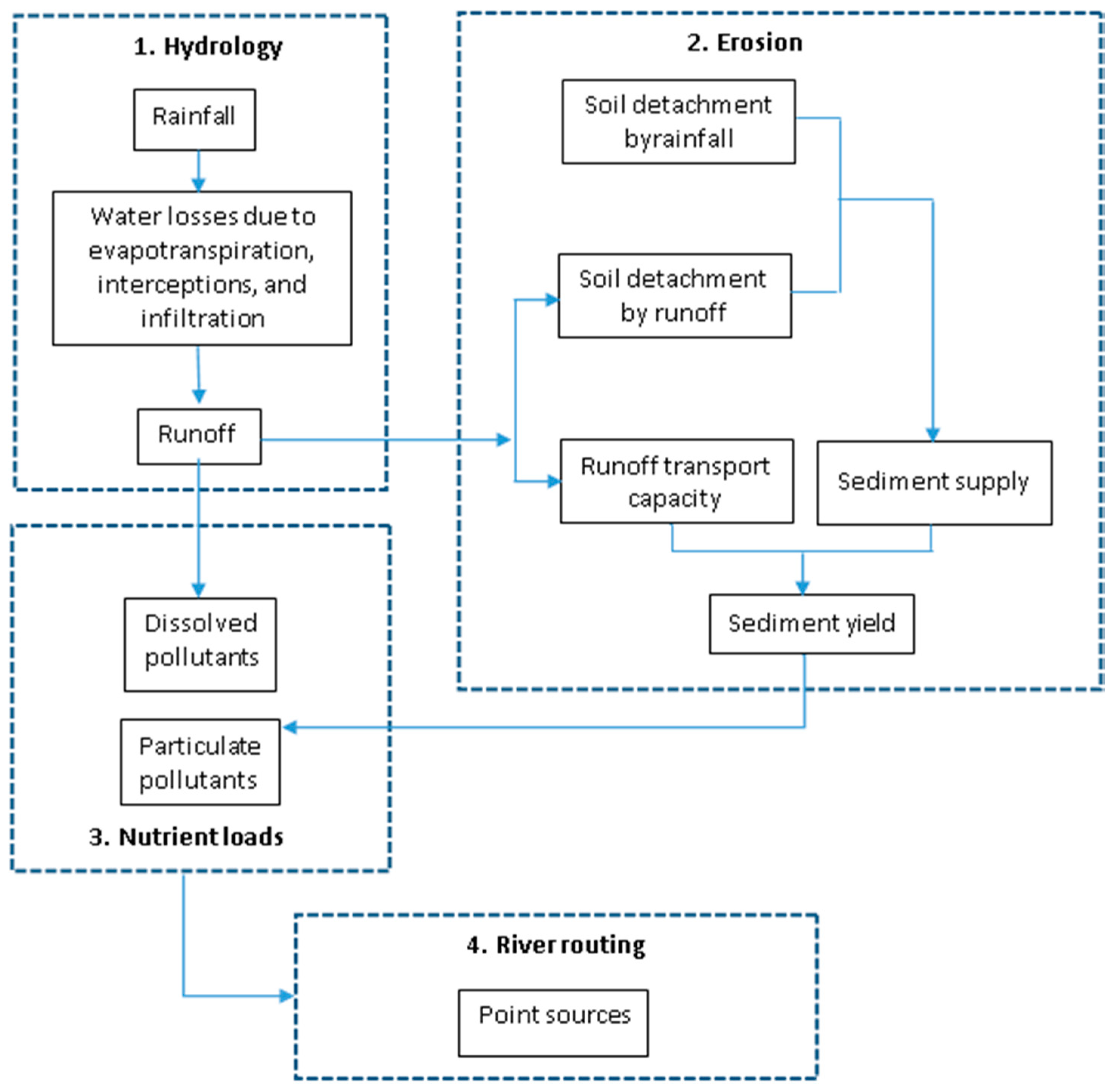
Figure 1. Scheme of the water quality model.
Sustainability 11 01773 g001
Figure 2. Variables in the Soil Conservation Service (SCS) method of rainfall abstraction (figure taken from Chow et al. [30], p. 147).
Sustainability 11 01773 g002
Figure 3. Description of river reaches as reservoirs (top); conceptualized connection of pollutant sources, sink, and changes within the reach and catchment (bottom) (adopted from Reference [46]).
Sustainability 11 01773 g003
Figure 4. A full water quality model merged in a spreadsheet.
Sustainability 11 01773 g004
Figure 5. Study area in three-dimensional (3D) view by draping with Landsat TM composite band 1, 2, and 3 (upper right) in relation to the Dong Nai river basin [48] (lower right; provincial borders are bounded by black line); location of the study area in Vietnam (left).
Sustainability 11 01773 g005
Figure 6. The Tra Phi catchment (rivers extracted from a digital elevation model (DEM) shown in light blue) and existing irrigation canals (shown in dark blue).
Sustainability 11 01773 g006
Figure 7. Regression of logarithm of the number of streams, average stream length, and average catchment area for the Tra Phi catchment.
Sustainability 11 01773 g007
Figure 8. Sub-catchment delineation based on DEM processing (left) and main river network and river reach discretization (~1000 m for each reservoir) (right).
Sustainability 11 01773 g008
Figure 9. Sensitivity analysis for nutrients after perturbing the hydrological and soil erosion parameters (left) and nutrient loading parameters (right).
Sustainability 11 01773 g009
Figure 10. Observed and simulated runoff flow discharge.
Sustainability 11 01773 g010
Figure 11. Observed and simulated results of total suspended solid (TSS) (a), and P-PO4 (b).
Sustainability 11 01773 g011
Figure 12. Observed and simulated results of N-NH4 (a), and N-NO3 (b).
Sustainability 11 01773 g012
Figure 13. Simulation results with uncertainty boundaries for TSS (a) and P-PO4 (b).
Sustainability 11 01773 g013
Table 1. Values of the number of streams, average stream length, and average area, as well as their expected values and the Horton’s ratios.
OrderC1_N
(number)
C1_L
(km)
C1_A
(km2)
C1_N_LSq
(number)
C1_L_LSq
(km)
C1_A_LSq
(km2)
Horton’s Ratio
RBRLRA
182.21.317.1272.5561.6392.831.834.00
226.3110.262.524.6736.555
317.3520.960.8918.54126.221
Table 2. Constant parameters.
ParametersNotationUnitsValues
Coefficient in transport capacity relationshipA 0.00066
Power in transport capacity relationshipB 1.61
Power in the depth–discharge relationship parameterB 1.667
Overland flow resistanceKf 130.3
Water specific weightΓkN/m39.80 × 103
Density of waterPkg/m31.00 × 103
GravityGm/s29.80
Shields sediment functionØ 3.76 × 10⁻²
Shields criterion Reynolds numberR* 4.66
Kinematic viscosity of waterNm2/s1.00 × 10−6
Table 3. Catchment parameters.
Slope (So)Area (ha)Overland Flow Length (m)
Sub 10.210266272.80
Sub 20.005811555.2
Sub 30.006389262.4
Sub 40.006621262.4
Sub 50.00287.960.0
Table 4. Soil and land-use parameters.
Sub-CatchmentD50 (*)σ (*)D (*) (kg/J)GC (*)CF (*)
Sub 10.00012.102.00 × 10−50.1–0.8(0.73) (**)0.35–0.9 (0.40)
Sub 20.00012.102.00 × 10−50–0.9 (0.55)0–0.9 (0.54)
Sub 30.00012.102.00 × 10−50–0.9 (0.68)0–0.9 (0.44)
Sub 40.00012.102.00 × 10−50–0.9 (0.47)0–0.9 (0.59)
Sub 50.00012.102.00 × 10−50.1–0.6 (0.47)0.5–0.9 (0.61)
(*): Look-up table (see Appendix); (**): min–max (aggregated values).
Table 5. Aggregated values of nutrient parameters.
CdktCsktTDkTSk
P-PO4N-NH4N-NO3P-PO4N-NH4
(mg/L)(mg/L)(mg/L)(mg/L)(mg/L)
Sub 10.00060.00040.020.110.051.000.305
Sub 20.00140.00100.040.250.121.000.314
Sub 30.00130.00080.030.230.101.000.240
Sub 40.00180.00110.050.330.131.000.310
Sub 50.00110.00110.050.20.131.000.371
Table 6. Tra Phi reaches/reservoirs information.
ReachLength (m)Number of ReservoirsAverage
Flow Velocity (*)—V (m/s)
Travel Time per Reservoir—T (hours)
1173810.640.75
2553650.480.64
3111010.640.67
4263930.480.51
5154410.400.77
(*): Average flow velocity obtained from field observations.
Table 7. Initial pollutant input from the sub-catchments (OC) (kg/h) (*).
Sub-CatchmentTSSP-PO4N-NH4N-NO3
Sub 1720.0540.0360.108
Sub 22160.1620.1080.324
Sub 3720.0540.0360.108
Sub 43600.270.180.54
Sub 519691.240.391.44
(*) reference: field observation.
Table 8. Model parameters used for sensitivity analysis.
AcronymsDescriptionRange
Hydrology
CNCurve number±20%
RainRainfall (mm)±20%
VoOverland flow velocity (GIUH module)±20%
VsAverage stream velocity (GIUH module)±20%
Erosion
KSoil erodibility factor±20%
D50Median size of soil particle±20%
PORPorosity of surface soil layer±20%
Nutrient Loading
Cdkt (N-NO3)N-NO3 concentrations in dissolved forms±500%
Cskt (P-PO4)P-PO4 concentrations in solid-phase forms±500%
Cskt (N-NH4)N-NH4 concentrations in solid-phase forms±500%
River Routing
VRiver reach velocity (Flow routing module)±20%
Point Sources
TSSTSS point sources (hourly)±500%
P-PO4P-PO4 point sources (hourly)±500%
N-NH4N-NH4 point sources (hourly)±500%
N-NO3N-NO3 point sources (hourly)±500%
Table 9. Statistical evaluation criteria for simulations from 25 to 27 July 2008.
NSEdR2PBIAS
Runoff Flow0.900.970.900.26
TSS0.200.830.6129.97
P-PO4−1.040.780.713.48
N-NH40.420.730.3312.02
N-NO30.100.760.4219.44
(Detailed descriptions of NSE, d, R2, PBIAS are shown in Table A3 of the Appendix).
Table 10. Variation (min–max of 5%) of model parameters for uncertainty analysis.
AcronymsDescriptionPdfApplied Values(min; max)
Hydrology
CNCurve numberUniform54(52; 56)
RainRainfall (mm)Uniform40.5(38; 42)
VoOverland flow velocity (GIUH module)Uniform0.04(0.03; 0.05)
VsAverage stream velocity (GIUH module)Uniform0.75(0.65; 0.8)
Erosion
D (K)Soil erodibility factorUniform0.14(0.1; 0.18)
D50Median size of soil particleUniform0.11(0.05; 0.15)
PORPorosity of surface soil layerUniform0.6(0.5; 0.7)
Nutrient Loading
Cdkt (NO3)N-NO3 concentrations in dissolved formsUniform0.08 (*)(0.02; 0.3)
Cskt (P-PO4)P-PO4 concentrations in solid-phase formsUniform1 (*)(1; 5)
Cskt (N-NH4)N-NH4 concentrations in solid-phase formsUniform0.2 (*)(0.04; 1)
River Routing
VRiver reach velocity (Flow routing module)Uniform0.8(0.75; 0.85)
Point Sources
TSSTSS point sources (hourly)Uniform50(30; 100)
P-PO4P-PO4 point sources (hourly)Uniform0.8(0.5; 1)
N-NH4N-NH4 point sources (hourly)Uniform0.6(0.4; 1)
N-NO3N-NO3 point sources (hourly)Uniform1.2(0.6; 1.5)
(*): multiplicity factor for each land use.
Table 11. Variation (min–max of 90% confidence) of constituents at different scenarios.
ScenariosFlowTSS PeakP-PO4 PeakN-NH4 PeakN-NO3 Peak
NSEmg/Lmg/Lmg/Lmg/L
1CN0.85–0.951600–34501–2.30.72–1.61.8–4.1
2CN, rainfall0.85–0.95700–30000.8–2.10.35–1.220.8–3
3CN rainfall, Vo0.85–0.951250–28200.78–1.620.55–1.20.12–2.95
4CN rainfall, Vo, Vs0.85–0.951450–31000.9–1.910.67–1.391.82–3.54
5CN rainfall, Vo, Vs, D(K)0.85–0.95750–25000.68–1.720.63–1.371.74–3.44
6CN rainfall, Vo, Vs, D(K), D500.85–0.951550–326500.92–1.870.82–1.562.15–3.86
7CN rainfall, Vo, Vs, D(K), D50, POR0.85–0.951160–28400.37–1.310.67–1.391.05–2.76
8CN rainfall, Vo, Vs, D(K), D50, POR, Cdkt (NO3), Cskt (P-PO4), Cskt (N-NH4)0.85–0.95810–26500.81–2.250.45–1.371.85–4.85
9CN rainfall, Vo, Vs, D(K), D50, POR, Cdkt (N-NO3), Cskt (P-PO4), Cskt (N-NH4), V0.85–0.95600–25300.85–2.120.41–1.251.23–2.51
10CN rainfall, Vo, Vs, D(K), D50, POR, Cdkt (N-NO3), Cskt (P-PO4), Cskt (N-NH4), V, point sources (TSS, P-PO4, N-NH4, N-NO3)0.85–0.951400–25001.1–1.80.42–1.21.15–2.8