Should I Stay or Should I Go? Assessing Intermodal and Synchromodal Resilience from a Decentralized Perspective

Abstract

Synchromodal transport incorporates real-time events in a dynamic manner in order to facilitate the most suitable selection of modes, routes and handling points. Up until now, current assessments rely on analytical models. Most of these models average distances for barges and trains via route mapping platforms that provide realistic distances for road only. To reflect on real-world developments more accurately, new thinking and modelling approaches are necessary to bridge academic models with physical transport processes. This paper introduces a computational model which computes movements of agents in geographically referenced space. The model captures stochastic parallel processes for each mode, and simulates decentralized delivery performance of each order in terms of cost, time and emissions at an operational level. Furthermore, we study the routing of individual orders and their responsiveness to disruptions. Computational experiments are performed within a case study which concerns imports of retail goods by unimodal truck transport from France to Belgium. Our findings show that dynamic synchromodal solutions cope with disturbances better, but unnecessary deviations and pro-activeness can also lead to negative effects when compared to static intermodal solutions

1. Introduction

The growing cargo demand, increasing road congestion as well as reliability, safety and environmental concerns have increased the relevance of more efficient and/or sustainable freight transport. By 2030, the ambition of the European Commission [1] is to shift 30% of freight transported by road to environmentally friendlier modes that have lower societal impact, such as rail and inland waterways. This shift should increase to 50% by 2050. Critical issues in this perspective are the modal choice preferences and transport mode selection [2,3,4]. The findings of the modal choice literature often yield higher user preferences related to road transport based on the user’s needs. Intermodal transport, which is a combination of two or more modes in one unified journey [5], provides more options and opportunities for a positive modal shift. However, the development of intermodal decision support models, where more actors and modes are incorporated (compared to unimodal), are hampered by limited data availability and its static nature [6]. Furthermore, shippers perceive intermodal transport as a slow and inflexible solution with a limited service offer [7].

Synchromodal transport/synchromodality presents an extension of intermodal transport by including real-time re-routing of loading units over the network to cope with disturbances and/or customer requirements [8,9]. The main difference between intermodal and synchromodal transport is that the former is based on services which are predefined long in advance, posing a rather static and inflexible service level. As a matter of fact, realistic problems and dynamics such as disturbances, breakdowns and other delays lead to time/money losses. Let alone, newly incoming orders cannot be accounted for in time as the intermodal setting is rigid. In the synchromodal setting, decisions related to modal choice and route are not predefined long in advance, but are taken as late as possible based on real-time infrastructural and operational developments [8]. Thus, the synchromodal concept has a potential to offer better performance than intermodal transport on flexibility, reliability and other modal choice criteria. This concept is to support optimal integration of different transport modes and infrastructure in order to address the earlier mentioned deficiencies and make intermodal transport more dynamic, flexible and acceptable. For a more detail overview of the synchromodal concept, we refer the reader to [10].

Synchromodality has also been regarded as a solution to congestion problems, decreasing reliability of services and environmental concerns caused by the growth of international trade and higher cargo demand [11]. In order to create a synchromodal transportation system, shippers should be convinced to book their transport requests mode-free. Mode-free booking, also called a-modal, provides an opportunity for logistics services providers (LSPs) to flexibly plan transport orders within the expected customers’ (shippers’) requirements by combining orders and using rail or inland waterway, rather than unimodal road-only transport. However, the synchromodal concept needs more quantification to demonstrate the benefits of having a dynamic and flexible network of services. In this regard, there is only a limited number of quantitative studies [12,13,14,15,16] and our paper is to contribute to this body of literature by using a computational approach. The motivation behind this is that analytical approaches assess freight systems from a central perspective, considering how the solution can work in the most efficient way for the given centralized system or a corridor, but little has been done from a decentralized perspective where the needs and objectives of cargo owners can be considered.

This paper presents a model that simulates the modal shift potential for hundreds of retail orders over a year. We assess the resilience of static intermodal and dynamic synchromodal solutions by computing alternatives in cases of disruptions which influence service reliability (early/late arrivals) cost and emissions. In fact, reliability is one of the main concerns of shippers and LSPs that hampers the potential use of intermodal transport [7,17]. To the best of our knowledge, a quantitative analysis assessing the resilience of intermodal and synchromodal chains to disruptions has not been addressed. In this paper we contribute to the current literature by providing a deeper understanding of modal shift potential in recovery settings.

We pose two main research questions: (1) what is the potential modal shift and emission reduction of individual dispersed orders served by truck-only when decentralized search algorithms are deployed? (2) Does synchromodal dynamic reconfiguration have any impact on the lead-time, cost and emissions compared to the more static intermodal setting under disruptions? The paper is structured as follows: Section 2 provides a brief overview of existing literature, Section 3 describes the methodological approach which is applied to a case study in Section 4. We convey the results also in Section 4 and discuss our findings in Section 5, followed by concluding remarks in Section 6.

2. Literature Review

Synchromodal literature is mostly exploratory and theoretical in nature [8,17,18,19,20,21,22,23,24,25,26,27,28,29]. Only a few studies provide quantification of the idea; ref. [12] present a mathematical model for designing integrated barge and train service schedules for synchromodal freight transport systems within the Rotterdam–Tilburg corridor. Another perspective is evaluated by [14] who propose a synchromodal planning algorithm used within a control tower for a 4PL logistics service provider. Ref. [15] developed a comparative analysis model for intermodal and synchromodal transport, taking into account economic, societal and environmental aspects. Ref. [13] assess service and transfer selection for different freight within a synchromodal network under uncertain demand by using a look-ahead approach. The revenue management aspect of synchromodality is addressed by [16] who focus on the cargo fare class mix problem to demonstrate that booking limits for differentiated fare classes at a tactical level lead to increased revenue. Synchromodal benefits from a supply chain perspective are studies by [30] who demonstrate an increase in intermodal rail transport share when taking into account more holistic supply chain impacts. The existing quantitative studies focus on synchronizing schedules and mode services, but little has been assessed at the operational level where the performance of individual orders is considered from a decentralized perspective. Current approaches to modelling synchromodality are based on analytical models [10] that do not fully consider the dynamic operational aspects such as real-time events, dynamic re-routing in geographical space, and resilience to disruptions. Most of these models average distances for barges and trains via route mapping platforms that provide realistic distances for road only. Even though there exist geographic information system (GIS) models that represent detailed inland waterway (iww) and rail distance measurements via shapefiles [31,32], these models cover the strategic (long-term) planning horizon such as terminal location analysis and market shares. Such analytical models use observables which are moved by the model in a top-down manner. These observables are mere numbers and do not possess any attributes and parameters that may govern the movement or interests of the studied entities from a bottom-up perspective. In reality, the movements of orders and modes are more independent and decentralized, governed by individual biases and order parameters such size, origin, destination, time windows etc. These parameters vary for each order which consequently yield different lead-times, costs, distances and emissions.

Disruption studies that take into account disruption management problems, resilience and recovery of freight transport networks, focus on long-term strategic assessments that concern responsiveness to bombs, terrorist attacks, floods, earthquakes and terminal attacks [33,34]. Only a limited number of studies consider the operational level, such as [35] who provide a disruption management method while considering road disruptions and their estimated duration. However, the work does not account for rail disruptions, and the analytical numerical example does not include any time and distance elements. Ref. [36] on the other hand, account for the time component but exclude transport cost and focus only on a single corridor. More recently, ref. [37] study disruptions in the physical internet context. The case study does not include terminals, terminal transshipments, pre- and post-haulage and iww alternatives. Our paper is to address these gaps by combining features of agent-based modelling, GIS and discrete-event modelling (further elaborated in Section 3). As far as the resilience term is concerned, we borrow the definition of resilience from [38] who describe it as an ability of an element to return to a pre-disturbance state, or move to a new one, after a disruption. To measure resilience, the status quo (non-disrupted system) will be compared to reconfigured solutions which will emerge when imposing various disruption profiles that may occur in reality. Such profiles will include disruption length, severity and probability of occurrence. By doing so, various mitigation strategies will be tested while taking into account how the devised mitigation strategies (re-routing, bundling, mode switching) perform in terms of key performance indicators (KPIs) (costs, emissions, lead-times).

Agent-based modelling presents a solution to capture behaviour of assets and their performance in recovery situations under disruptions. Agent-based models (ABM) have a very high potential as a result of the advancements in object-oriented programming languages in computer science that have the ability to represent heterogeneity in physical and human systems [39]. ABM include heterogeneous agents with different knowledge of their environment and layouts [40]. Agents may represent trucks, trains, barges, orders, terminals and various other entities. These entities have the ability to self-organize locally which may lead to significant reconfiguration of relationships and processes based on internal perturbations or external shocks [41]. Since agents are local, they monitor the value of system variables locally as well, without averaging and thus without losing the local idiosyncrasies or individual specificities that can determine overall system behaviour [42]. Agents can process and exchange information with other agents as well as perceive other entities, obstacles or sense their surroundings [43]. Such agent characteristics allow for simulating behaviour of assets from a decentralized perspective which is why our methodology, in the following section, builds on this modelling approach. In terms of freight transport and ABM applications, ref. [44] focus on agent interaction by simulated contracts while considering road and short sea shipping. A participatory simulation gaming approach in an urban freight transport context is studied by [45]. The agent entities are depicted as decision-makers which does not fully exploit the possibilities of autonomous and decentralized agent routing strategies and consequent distance collection in case of deviations induced by disturbances. Lastly, the work of [46] assesses the impact of the transalpine rail network disruption by using ABM.

Our work is to make use of all the above listed research progress and combine synchromodal and disruption advances as well as advances in agent-based modelling. In other words, this paper studies disruptions in a synchromodal context by using agent-based modelling. The paper contributes to (1) advancing modelling approaches and (2) better resilience assessments where we do not take actual freight movement as exogenous parameter inputs. We consider the geo-spatial context that governs movements of barges, trucks and trains from a decentralized perspective in order to capture different emerging patterns once assets are re-routed or delayed.

3. Methodology

Current synchromodal analytical models [10] optimize corridor flows which increases efficiency in terms of cost and time for a given corridor of already existing rail and iww services. To achieve the modal shift objectives mentioned in the introduction, models should also be designed for convincing shippers who have not yet tapped into the rail and iww solutions. Therefore, decision support models should account for supplier origins (O) and delivery destinations (D) that are dispersed in geographical space. Hence, each order, OD, pair has different spatial attributes which yield different distance and lead-time values. ABM incorporate different scale and time processes into a single simulation as the time steps are discrete and small enough to approximate real-time dynamics [43]. In this regard, ABM computer simulations can offer substantial benefits as they allow for execution of parallel processes such as different mode adaptations to multiple disruptions. The main novel aspects of our model are the following:

• decentralized agent process (bottom-up) simulations of each order/container and the modes it undergoes, as well as order performance in terms of distance, time, cost and $C{O}_2$.
• more realistic routing strategies through geographically referenced space for trucks, trains and barges in a single model.
• disruption and system resilience assessment by decentralized reconfiguration of solutions induced by messages and spatial awareness.

3.1. Representation of Space and Time

Different types of problems lead to different types of models and formalism. While most synchromodal models rely on linear programming approaches that function in mathematical abstract space, agents need to be spatially aware of their surroundings. The main modelling canvas of our SYnchromodal Model for Belgian Inland Transport (SYMBIT) is a digital map that comprises of road, rail and iww vector files. The vector files, also called shapefiles, are acquired from ETISplus which is the European Transport policy Information System, and Eurogeographics. The vector data files contain the TEN-T networks for roads, railways, airports, ports and the watercourse system identified by Directorate-General for Mobility and Transport (DG MOVE). As indicated in Figure 1 (top-right), the cyan coloured polylines represent navigable iww and railway shapefiles. The latter concerns freight priority links. The other dark image under depicts all geocoded locations of European ports and inland terminals. Each location contains attributes with regard to mode switching possibilities and terminal size. The GIS environment presented herein provided our agents with real-world locations based on the WGS84 geographic coordinate system, having Greenwich (0, 0) as its prime meridian. The reason behind choosing the WGS84 coordinate system is its broad application; used as a reference system by GPS, Google Maps as well as by Microsoft in its Bing Maps. This digital infrastructure is part of the transport supply that also includes existing services and schedules that induce agent movements. The schedules and services were validated via the Intermodal links and Contargo platforms.

Synchromodality encompasses uncertainties due to the wide range of external inputs that may affect internal resource states. These inputs occur dynamically and in real-time. In this regard, dynamic models can effectively capture state fluctuations over time [47] which is why a computation modelling approach is chosen to capture the synchromodal dynamics in simulated real-time. As dynamic models can be time-driven and event-driven, the latter represents a better fit as nonlinear evolution of the model in continuous time would not account for real-time dynamics. The ABM approach herein is represented as a discrete-event system (event-driven). The state of agents is affected by the occurrence of events over time as they roam through the geo-referenced space.

Figure 2 represents a flow of an order starting at an origin node to a destination node DC (Distribution Center). Once a moving agent enters a stationary agent, it is transformed into an entity and becomes a part of the stationary agent’s processes that are organized in a discrete event logic; for instance, container transshipment at a terminal. When the process is finished, the entity re-emerges as an agent. SYMBIT continuously monitors the state of agents from the point when the order is sent to the origin which represents a supplier. It then logs the type of transport means the order is carried by, covered individual distances, elapsed time, terminal handling and dwelling time, and last-mile delivery which stops the monitoring process of a specific order at TimeMeasureEnd.

3.2. Model Formulation

The model works with the following sets, parameters and variables:

• $M=\{0,1,...,n\}=$ array list of transport means m representing trucks, barges and trains
• $H=\{0,1,...,o\}=$ array list of terminal agents h
• $S=\{0,1,...,p\}=$ array list of supplier agents s
• $DC=\{0,1,...,x\}=$ array list of distribution center agents $dc$
• $O=\{0,1,...,s\}=$ array list of order agents
• $N=\{0,1,...,q\}=$ vector file of nodes
• $L=\{0,1,...,w\}=$ vector file of links representing rails, inland waterways and roads
• $m^c=$ cost per km of m
• $h^c=$ handling cost at terminal h
• $h^t=$ handling time at terminal h
• $h^s=$ storage cost at terminal h
• $o^{s,dc}=$ individual order to be transported from $s\in S$ to $dc\in DC$
• $l{d}^o=$ lead-time of an individual order $o^{s,dc}$
• ${\lambda }_o=$ allowed time window per order
• $s^m=$ average speed of m in km/h
• $d_{\left|\right|i\to i+1\left|\right|}^m=$ distance for a specific m from current i to next $i+1$ network node in GIS space
• $t_{\left|\right|i\to i+1\left|\right|}^m=$ transit time of m from i to $i+1$ network node in GIS space
• ${\ell }^m=$ load factor of m with $o^{s,dc}$ on board
• ${\xi }^m=$ emission factor of m per km
• ${\xi }_{s,dc}^o=$ emissions emitted for an $o^{s,dc}$ delivery
• $O_{s,dc}^c=$ total cost of an order
• $O{O}_{s,dc}^c=$ Total cost of all orders
• $D{T}_{s,dc}^o=$ Aggregated distances generated by order $o^{s,dc}$ movements
• $T{\xi }_{s,dc}^o=$ Overall emissions by all orders

The objective is to minimize $O_{s,dc}^c$ of an individual order $o^{s,dc}$ consisting of $m^c$ which is different for truck, barge and train as well as handling cost $h^c$ at loading and unloading location of $h\in H$. The $d_{\left|\right|i\to i+1\left|\right|}^m$ values are collected by each m agent when traversing $l\in L$ in simulated real-time. The $\left|\right|.\left|\right|$ expression, known for defining euclidean distance in euclidean space, is adapted to define realistic physical distances in the so called GIS space (geo-referenced space specified by GIS). Final values are aggregated upon $o^{s,dc}$ arrival at its distribution center which represents the final location (Equation (1)).

$$O_{s,dc}^c=\sum _{i\in N}{m}^c{d}_{\left|\right|i\to i+1\left|\right|}^m+h^c+h^s$$

(1)

$${\xi }_{s,dc}^o=\sum _{i\in N}{\xi }^m{d}_{\left|\right|i\to i+1\left|\right|}^m.$$

(2)

To obtain emission values emitted by each order delivery ${\xi }_{s,dc}^o$, the combination of m agents and their individual performances in terms of covered distances $d_{\left|\right|i\to i+1\left|\right|}^m$ were considered (Equation (2)). The emission factor ${\xi }^m$ that corresponds to the specific m was then applied to its covered distance. Only distances travelled with the order on board were taken into account. Return trips of modes were not included.

The lead-time of an order $l{d}^o$ depends on the performance of individual m agents that can be faster or slower based on the infrastructure $l\in L$ they follow. Equation (3) depicts transfer times $t_{\left|\right|i\to i+1\left|\right|}^m$ for each m while considering their speed $s_k^m$. The order lead-time $l{d}^o$ is then acquired by including handling time $h^t$ in Equation (4) at loading and unloading terminals.

$$t_{\left|\right|i\to i+1\left|\right|}^m=\sum _{i\in N}\left(\frac{d_{\left|\right|i\to i+1\left|\right|}^m}{s^m}\right)$$

(3)

$$l{d}^o=\sum _{i\in N}{t}_{\left|\right|i\to i+1\left|\right|}^m+h^t.$$

(4)

The main decision variables were order cost $O_{s,dc}^c$ and order lead-time $l{d}^o$ that may be affected by external perturbations (disruptive events) that are labelled as $\Psi$. These external events induce re-routing strategies of m in GIS space which will, as a consequence, alter the delivery performance in terms of $O_{s,dc}^c$ and $l{d}^o$. Figure 3 illustrates a stochastic disruption input ${\Psi }_t$ at a given time t into ongoing processes of m is simulated real-time. The model tests control policies given the current system state $\eta \left(s_t\right)$ by sending out messages $m_t$ to re-route or switch to another mode while traversing $l\in L$. Our work focused on such control policies and their implications in terms of order costs $O_{s,dc}^c$, lead-times $l{d}^o$ and emissions ${\xi }_{s,dc}^o$. Such policies and their consequences may be of interest to LSPs, shippers, corridor managers and policy makers when evaluating and/or considering dynamic synchromodal processes.

The final aggregated outputs that our model delivers are shown in Equations (5)–(7). Total costs, lead-times, travelled distances and emissions are the KPIs. The following section provides more specifics in terms of parameter values and control policies $\eta$ where their impact on the KPIs is studied.

$$O{O}_{s,dc}^c=\sum _{k=1}^m{O}_{s,dck}^c$$

(5)

$$D{T}_{s,dc}^o=\sum _{k=1}^m\sum _{i\in N}{o}_k^{s,dc}{d}_{\left|\right|i\to i+1\left|\right|}^m$$

(6)

$$T{\xi }_{s,dc}^o=\sum _{i=1}^n{\xi }_{s,dci}^o.$$

(7)

As SYMBIT is not a linear programming model but a computational one, modelling constrains and operating principles will be listed in flowcharts and pseudo-codes provided in Section 4 and the Appendix A. The above equations are to illustrate how KPI values are accumulated when truck, barge and train agents start re-routing; hence, generating different values given their individual spatial and temporal context.

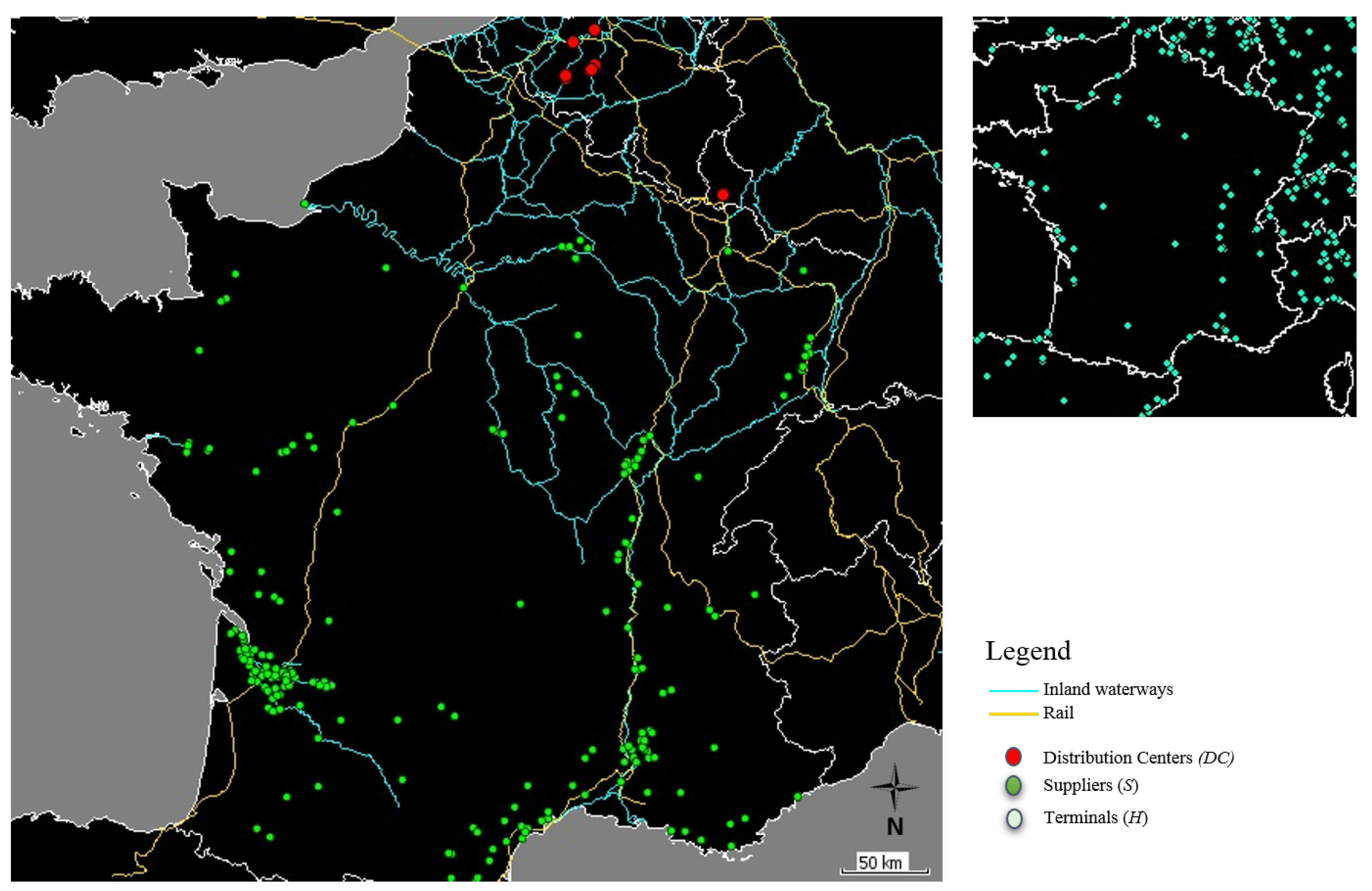
4. Application

The case study concerns imports of goods of a single retailer by unimodal truck-only transport from France to Belgium (Figure 4). A pool of LSPs provide a service to this retailer to transport payloads from 220 origins (S) to six destinations ($DC$). Demand/order generation in our simulations was based on these existing unimodal order flows. The order $o^{s,dc}$ parameters include a reference number, FTL or partial load, driver, week number, supplier location (latitude/longitude) and final DC location (latitude/longitude). Order placement started when the real-time simulator entered a new week. When the simulator entered week three for instance, all order requests that correspond to week three will be sent out to their S locations.

As far as general assumptions and parameter input values are concerned, the model considers trains which operate five times per week (closing time for transshipment is at 17:15) and barge services three times per week alongside the Rhine–Alpine corridor. Terminal operating hours are Monday–Friday between 07:00–19:00 and on Saturday between 07:00–12:00. Orders that arrive after train/barge departures will be transported on the next day.

Table 1. Parameter overview of moving and stationary agents.

Moving Agents	Truck	Barge	Train
$s^m$	60 km/h	5 knots (9.3 km/h)	50 km/h
${\ell }^m$	100% (2 TEU)	70% (85 TEU)	80% (70 TEU)
$m^c$ (fixed + variable)	€0.96	€0.21	€0.62
${\lambda }_o$	Five work days. Two work days for urgent order requests
${\xi }^m$ in CO${}_2$-${}_{eq}$ (CO${}_2$-${}_{eq}$ per order)	72 g/tkm (2060 g/km)	Downstream 23 g/tkm (657 g/km)	Electric 14 g/tkm (400 g/km)
Stationary/Terminal agents	Small	Medium	Large
$h^c$ at 60% utilization	€81	€60	€38
$h^c$ at 80% utilization	€61	€45	€28
$h^c$ at 100% utilization	€49	€36	€23
$h^s$	First 24 h (overnight stay) is free of charge

depicts specific values of the model’s parameters. Barge average speed $s^m$ is sampled from downstream flows of barges from marinetraffic.com. As for trains, according to the European Court of Auditors (ECA) the average commercial speed of freight trains in the EU is very low, only around 18 km/h on many international routes [49]. However, the ECA points out the average speed on rail freight corridors is comparable to the speed of trucks. Variable and fixed costs that compose cost per km $m^c$ are taken from LSPs which provided us with their data within previous projects. These include rail, barge and truck operators. The load factor ${\ell }^m$ determines $m^c$. Varying load factors, such as higher ${\ell }^m$ resulting in lower $m^c$ for trains and barges, are not considered for simplicity purposes. $C{O}_2$ equivalent factors (well-to-wheel) are taken from the STREAM freight transport 2016 report and are adjusted to two TEU per order. Gross weight of one TEU was set to 14.3t (2.3t tare + 12t payload) as indicated by [50]. Thus, one order (2TEU) weighs 28.6t. Terminal handling cost $h^c$ differentiation was based on the work of [51]. As far as transit times and distances between nodes are concerned, agents generate and record their individual distances ad hoc, together with the time they take to traverse the links. These values depend on the taken routes defined by shape-files (vector files):

• truck agents were governed by a road shape-file (main roads—fastest route A* algorithm).
• barge agents followed an inland waterway shape-file (navigable waterways—Dijkstra algorithm).
• train agents were linked to a railway shape-file (TEN-T corridor—Dijkstra algorithm).

Given the decentralized nature of agents, the ongoing delivery processes may reconfigure depending on the geographical location of the disruption, without unnecessarily bothering other agents and their ongoing processes. In this paper, we considered more short-term disruptions $\Psi$ by introducing three disruption profiles (

Table 2. Disruption profiles and their severity.

$\Psi$	Description (Example)	Probability of Occurrence per Year	Duration
1	Frequent and short (Delays caused by detours, blockages, light accidents, road works, etc.)	30–40%	Uniform (1, 3) h
2	Less frequent and short (Breakdowns, maintenance, moderate weather conditions, trees on rails etc.)	6–9%	Uniform (3, 6) h
3	Less frequent and mid-long (Strikes, severe weather conditions, floods, train collision, derailment etc.)	6–9%	Uniform (1, 3) d

). Profile 1 ($\Psi 1$) is applicable to road only, to simulate the overall delivery performance of intermodal orders if a truck arrives late, or not-depending on how far the individual trucks are from terminals. We assumed that these disruptions, slightly more severe than daily congestion, last 1–3 h. Profiles 2 ($\Psi 2$) and 3 ($\Psi 3$) occurrence estimations are deduced from Eurostat for rail only. Iww accident data were not available, which is why this study was limited to mainly rail disruptions. Profile 2 duration was taken from [36]. We use many model realizations with Monte Carlo simulations to approximate the stochastic probability distributions. During each realization the model draws a different value from the probability range.

4.1. Experimental Design

At the model verification stage, the agent code and routing were assessed by comparing our routing solutions with Google maps and Bing maps. This was to verify the correctness of distance accumulation per agent via road. For inland waterways and rails, the polyline lengths were inspected via ArcMap. The next step was calibration; after examining the distance correctness, the speed parameters were calibrated to meet realistic movements throughout the shapefiles. We considered congestion levels from google maps and automatic identification systems (AIS) that provide real-time vessel positions and their historical speeds. The variable cost/km for trucks was calibrated since the parameter can be tuned to improve agreement with observed truck data provided by our retailer. As we do not possess experimental data for waterborne and rail transport from the retailer, computational simulations are used to foretell the potential of those deliveries based on the fidelity of simple physics. 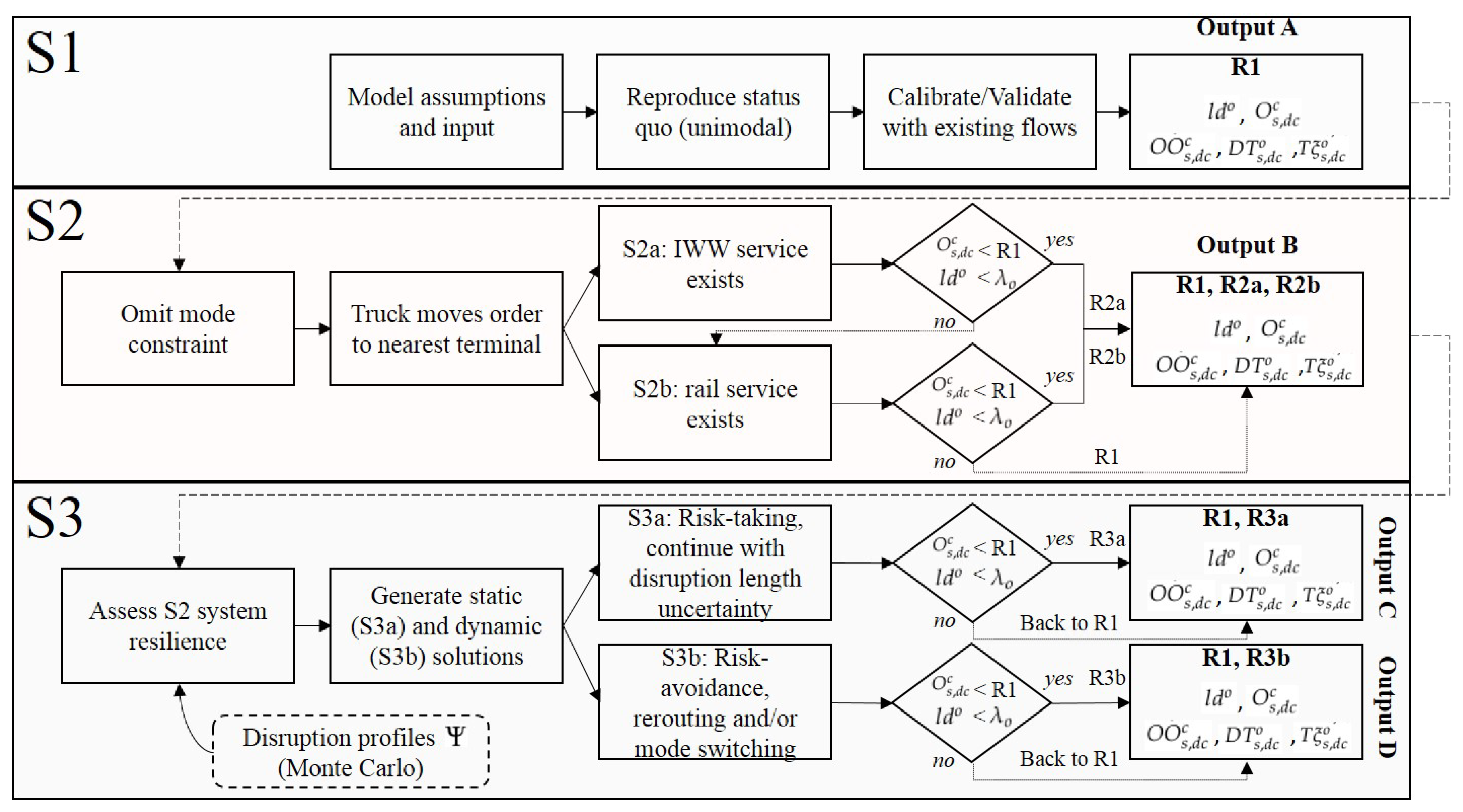Figure 5 provides a schematic overview of three main simulations.

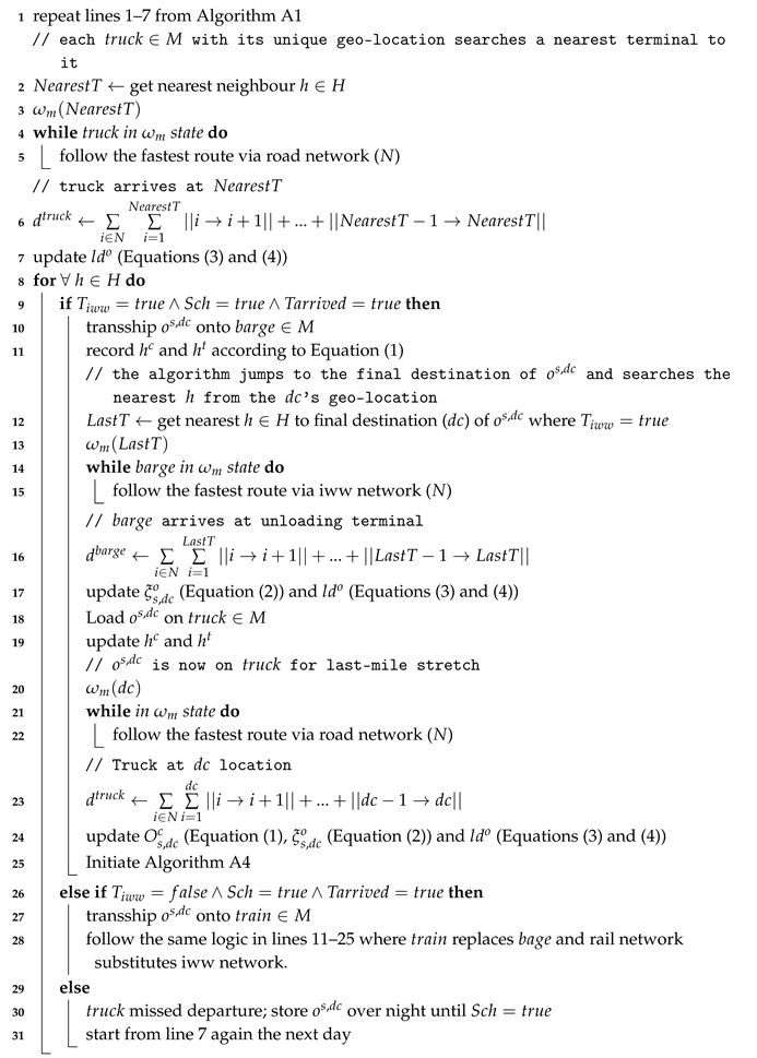
Simulation 1 $\left(S1\right)$—unimodal simulation (status quo): a dispatching loop scans the order file and sends out orders based on week numbers. Truck agents collected the orders at their geolocations in France at 08:00 and depart to the order’s DC locations in Belgium via geo-referenced space. The output values were indicated as output A in Figure 5. The calibration procedure yielded a cost of 0.87 Euro per km when final simulated deliveries were compared to existing data of the retailer. Therefore at this step, the truck cost/km input parameter $m^c$ is changed from 0.96 to 0.87. Appendix A.1 contains more details with regard to the computational logic of simulation 1.

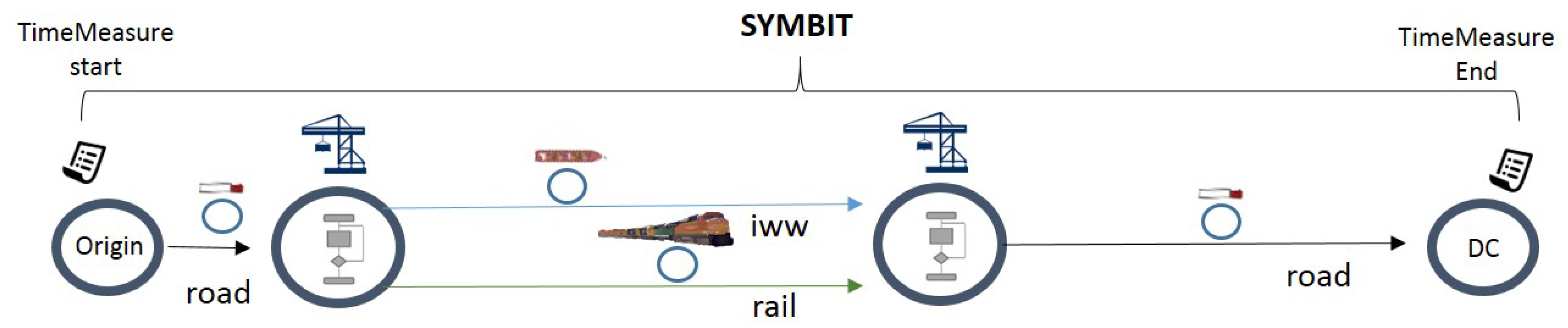
Simulation 2 $\left(S2\right)$—a service is booked rather than a single mode. The truck agents initiated a nearest neighbour search from their individual geolocations and depart to their nearest terminals for transshipment. Should there be a cheaper terminal within 50 km radius r (determined by $h^c$ of the terminal), the truck agents will move to $h\in H$ with the lowest cost. The order agent $o^{s,dc}$ was placed on a barge agent which receives the next terminal delivery location; an algorithm scans the DC geolocation embedded in $o^{s,dc}$ and searches the nearest cheapest terminal to that DC location in Belgium. The barge agent departs to that specific terminal and records its lead-time ($t_{\left|\right|i\to i+1\left|\right|}^m$) and cost ($m^c{d}_{\left|\right|i\to i+1\left|\right|}^m$) in Equation (1). The order agent is then transshipped to a truck for last-mile delivery. The pre-haulage—transshipment—main leg by barge—transshipment—post-haulage form the total cost of an order $O_{s,dc}^c$ and determine its lead-time $l{d}^o$. Both were then compared to result 1 (R1) from the previous simulation. If the time was lower than the allowed time window ${\lambda }_o$ and the cost was lower than the previous unimodal delivery of the specific order, the solution is kept as R2a. Else, if the cost $O_{s,dc}^c$ was acceptable but the lead-time ${\lambda }_o$ was exceeded, a rail solution is queried following the same procedure as above. If the rail result R2b was cheaper and deliverable within ${\lambda }_o$, the result was kept (Figure 5), if not, the initial R1 was kept. The same procedure was followed in case no iww service exists. Appendix A.2 sheds more light on the modelling logic.

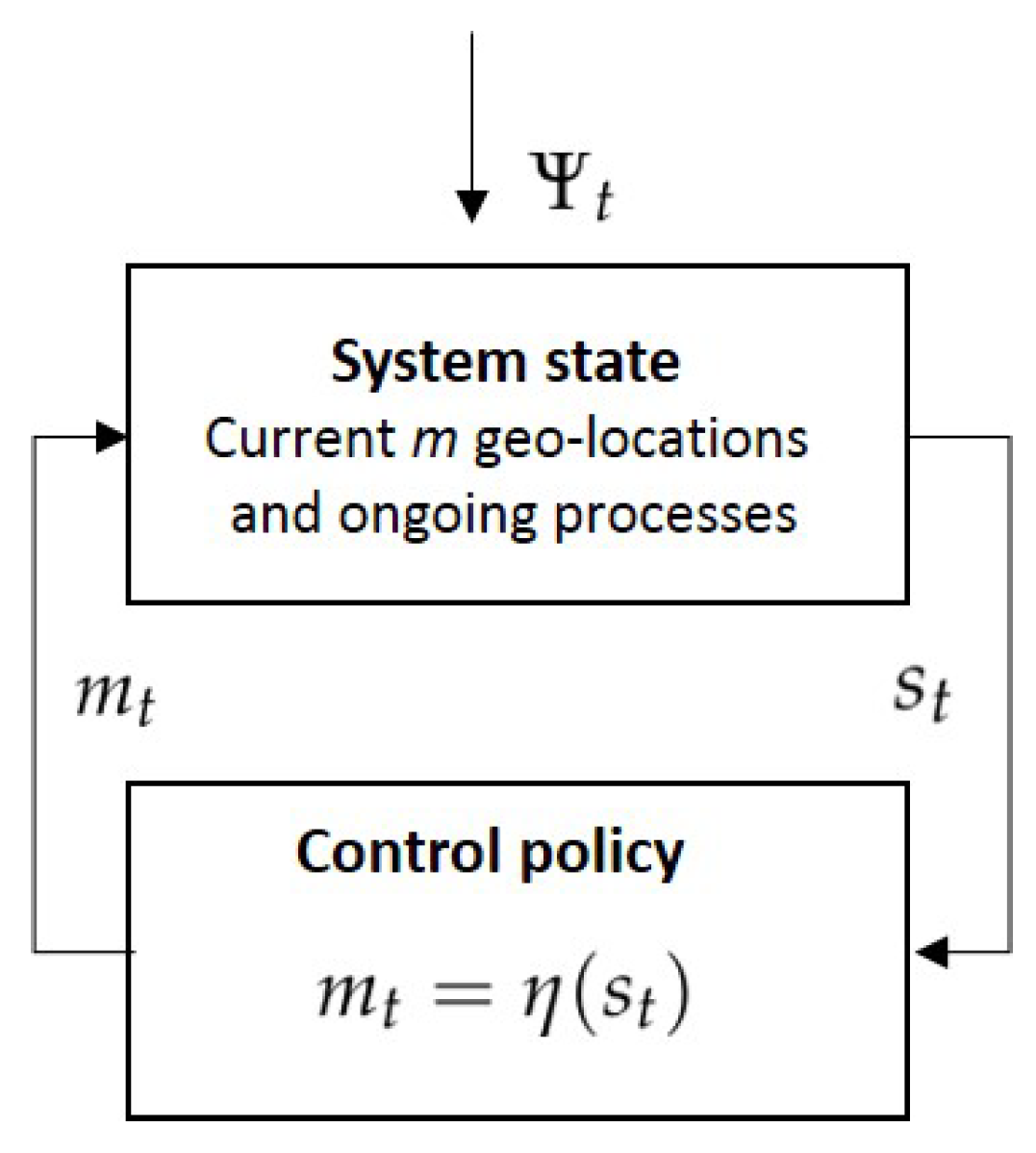
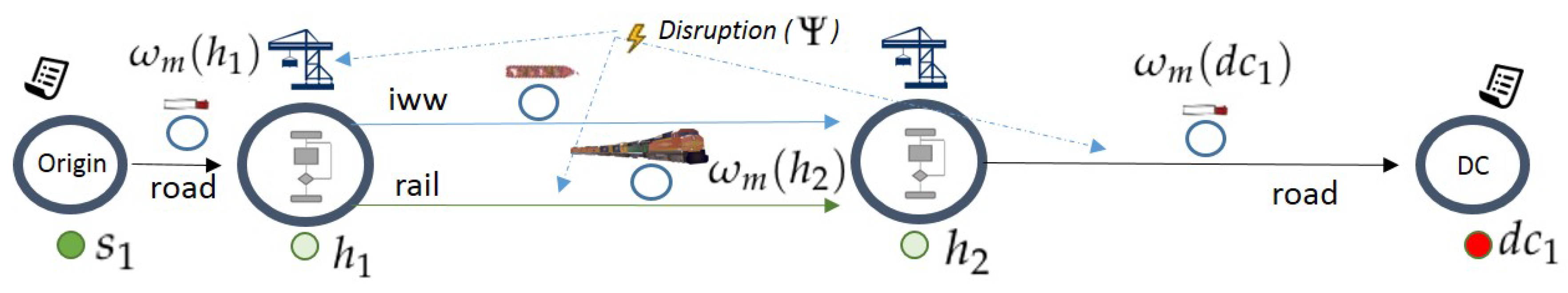
Simulation 3 $\left(S3\right)$—disruption scenario (resilience assessment): this simulation took the final configuration of S2 as its input, and tested the system resilience to perturbations. Having established intermodal solutions at this point, we focused on the flexibility aspect of synchromodality. We compare the intermodal (static) solution with the synchromodal (dynamic) solution. These two represent the control policies ($\eta$). The former, static, was labelled as risk-taking (Figure 5) which means that once the disruption profiles $\Psi$ from Table 2 were applied, all the agents in transition state ${\omega }_m(.)$ were be exposed to delays caused by $\Psi t$ given their current geolocations in space and time at the moment of occurrence (Figure 6). In the static case (S3a) the agents were delayed without knowing the disruption length. If the cost ($O_{s,dc}^c$ from S1) and time ${\lambda }_o$ thresholds were violated, the initial R1 solutions was kept. The latter, dynamic (S3b), means that agents received information about each disruption and proactively seek alternatives, labelled as risk-avoidance. Mainly disruption profiles 2 and 3 were considered since profile 1 did not have any significant impact on the deliveries (further elaborated in Section 4.2). Planning was done as late as possible so that the planners had enough time to detect disturbances and respond to them proactively. For profile 2, the trains were able traverse a path in case of terminal breakdown. This resulted in re-routing where the truck agent will move to the next nearest terminal. A search radius of 300 km was added to query iww terminals first. This was to find potentially cheaper options and also avoid trucks seeking rail terminals further inland in the opposite direction. The radius applied to orders situated within the Rhine–Alpine corridor which were closer to Basel in Switzerland. If the cost and time thresholds were not met, the R1 solution was reinstated. For longer-term disruptions in profile 3 such as rail strike, the LSP will seek other than rail alternatives. R3b is recorded in output D if cost was lower than R1 and time fell under five days (${\lambda }_o$). Else, R1 was reinstated. The static case output C was then compared to the dynamic case output D. The algorithm is described in more detail in Appendix A.3.

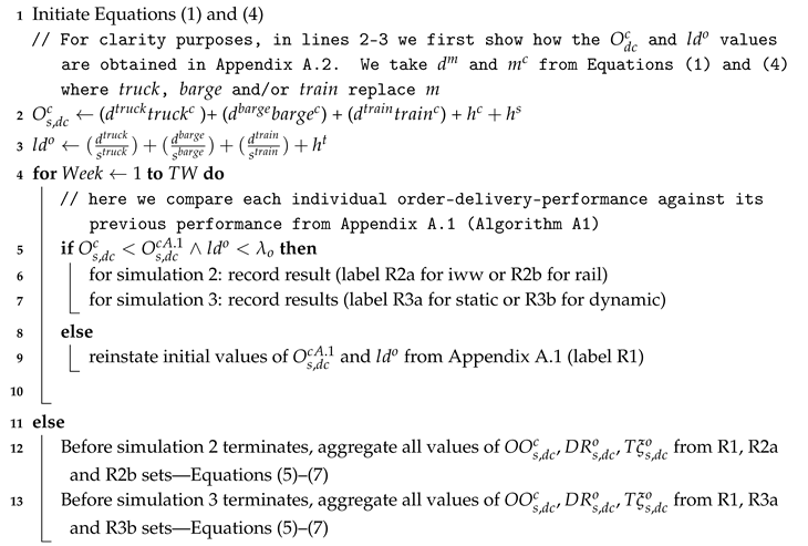
4.2. Simulation Results

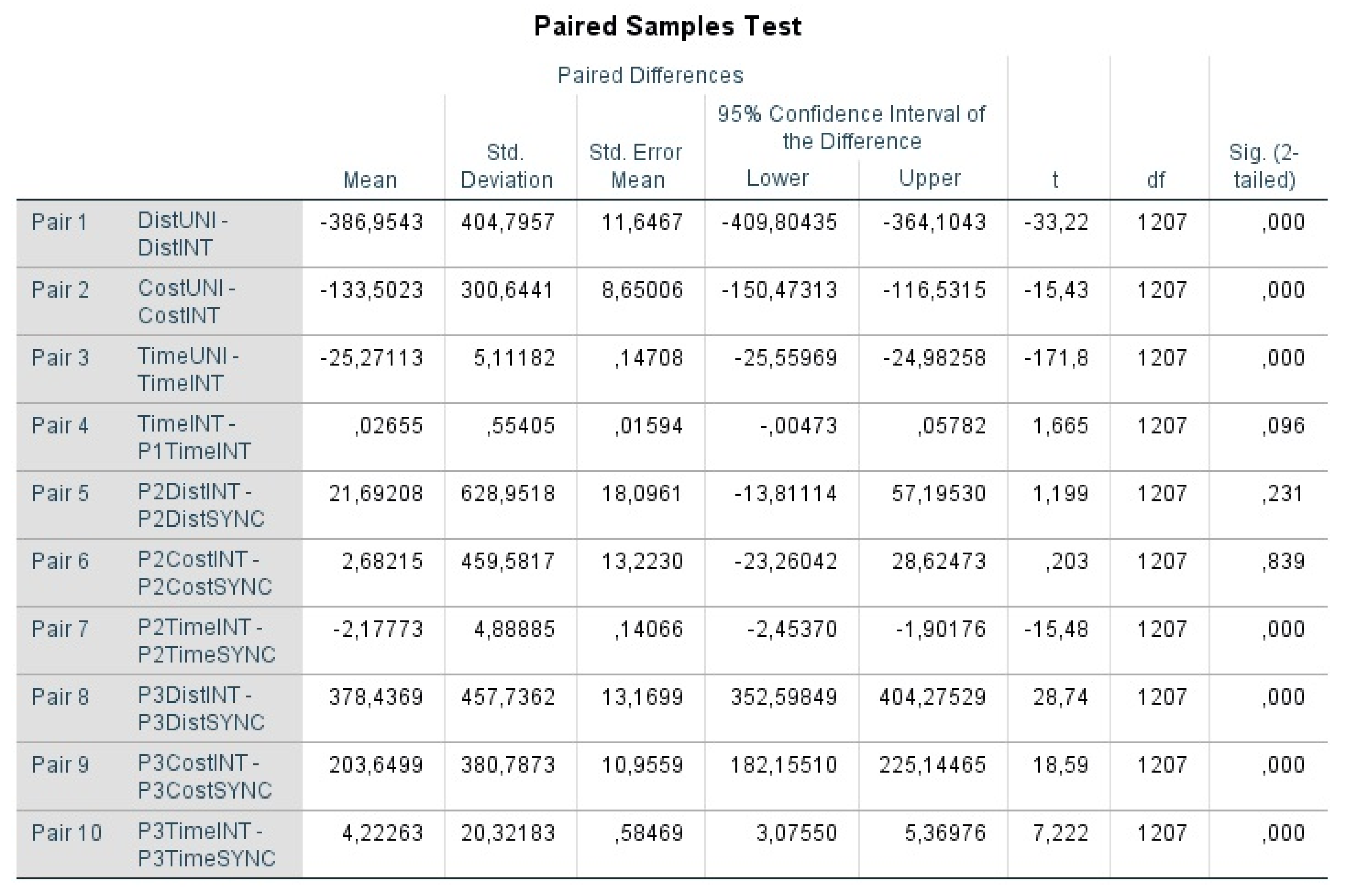
The case study results were validated with the retailer on a continuous basis; we have re-visited the retailer three times after each model calibration in order to validate with them whether the model represents realistic outputs. After each visit, we incorporated feedback provided by the retailer to increase the accuracy and validity of our model. The retailer provided us with their price files for truck-only deliveries. The output was analyzed statistically by using paired samples t-tests (Appendix B). We interpret the statistical difference in the following sub-sections. Significance level of 0.05 (p-value) was used which relates to confidence intervals of 95%. The analysis in Section 4.2.1 concerns our first research question, whereas Section 4.2.2 concerns the second research question.

4.2.1. Unimodal vs. Intermodal (Simulation 1 vs. Simulation 2)

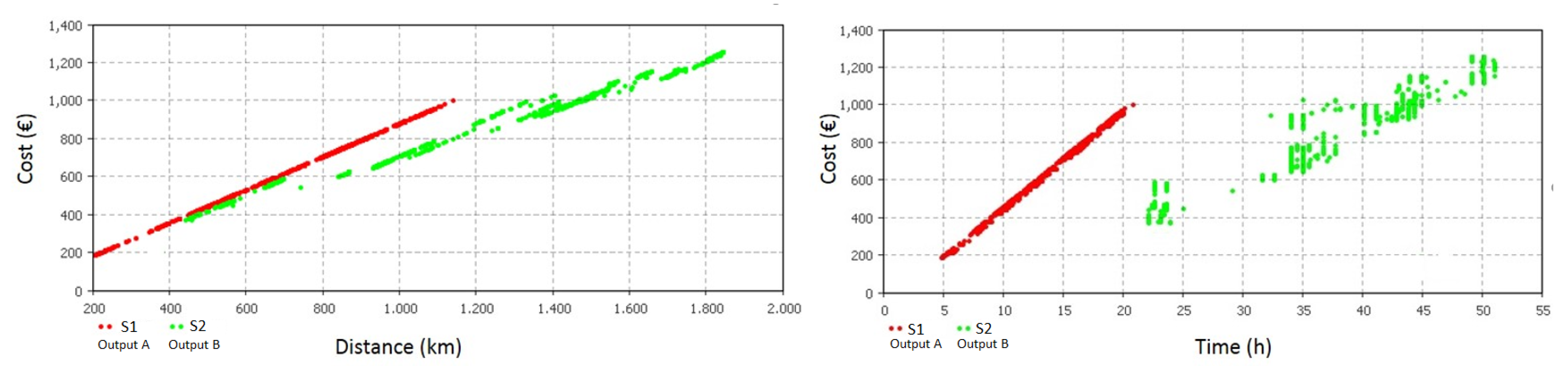
The results of simulation 1 and simulation 2 were shown in Figure 7 where the reproduced unimodal flows (red) were compared to computed intermodal flows (green). Each dot represents a single order $o^{s,dc}$ after reaching its final destination. The order plots indicate cost ($O_{s,dc}^c$), distance and lead-time ($l{d}^o$) per order that were recorder upon arrival at distribution centers. It can be visually inferred that intermodal options lead to longer distances, lead-times and higher costs. The cost increase is caused by extra handling and the containers need to be transshipped onto a barge or a train. The order costs in the interval between 800 and 1200 km were the most competitive as the lower cost per km of barges and trains compensated for the extra handling costs. Even though longer distances favoured intermodal transport, there were also flows that exceed €1000 and 1200 km (green). This was caused mainly by the first-mile of the trucks that take detours to their nearest terminals. Such detours, and also terminal handling operations, increased overall lead-times as illustrated in the right side of the figure. The differences per variable were significant: distance (p ≤ 0.05), cost (p ≤ 0.05) and time (p ≤ 0.05).

Table 3. Output for business-as-usual simulation (S1) and possible intermodal alternatives (S2).

	${\mathit{\lambda }}_{\mathit{o}}$ (Days)	Shifted/Unimodal (%)	Distance Share (%) (Road/Iww/Rail)	Cost Share (%) (Road/Iww/Rail/Term)	CO2-eq Share (%) (Road/Iww/Rail)
S1	${\lambda }_{o2}$	0/100	100/0/0	100/0/0	100/0/0
	Total${\mathit{\lambda }}_{\mathit{o}\mathbf{2}}$		887,110 km	€771,785	1,827,446 kg
S2	${\lambda }_{o5}$	26.5/73.5	79.1/4.3/16.7	83.1/1.1/12.5/3.3	94.5/1.6/3.9
	${\lambda }_{o2}$	14.5/85.5	84.7/0/15.3	87.1/0/11.2/1.7	96.6/0/3.4
	Total${\mathit{\lambda }}_{\mathit{o}\mathbf{5}}$		887,337,km	€734,331	1,529,276 kg
	Total${\mathit{\lambda }}_{\mathit{o}\mathbf{2}}$		906,355 km	€767,258	1,637,542 kg

shows simulation output A and B (as shown in Figure 5). When applying time window ${\lambda }_{o2}$ constraint of two days for S1, all trucks were capable of reaching their destination within that specific time frame. This fact was also validated by the retailer. The unimodal freight deliveries (truck-only) generated 887,110 km in one year which resulted in 771,785 of costs and 1,827,446 kg of CO${}_{eq}$ emissions. S2 yielded a potential of 26.5% of orders that can be shifted from road-only transport where 4.3% of distances were done via iww and 16.7% by rail. Even though the cost was distributed among roads, iww, rails and terminals, the combination still offers costs savings of €37,454 and an emission reduction of 298,170 kg on a yearly basis. When imposing ${\lambda }_{o2}$ instead of ${\lambda }_{o5}$, the share of shifted orders decreases to 14.5%. This percentage consists of orders that are geographically close enough to meet the time and cost constraints; carried by road and rail as depicted by the distance share in Table 3.

4.2.2. Resilience Assessment—Intermodality (S3a) vs. Synchromodality (S3b) Simulations

In this section, intermodal and synchromodal performances are compared when exposing S2 configuration to our disruption profiles (see Figure 5). Only profiles 2 and 3 are addressed since profile 1 did not have any significant impact (p ≥ 0.05); this means that 1–3 h delays did not affect the trucks which managed to reach their nearest terminal before train and barge departures. The profile input values from Table 2 that affect the behaviour of the system are based on Monte Carlo simulations. To ensure comparability, each simulation is executed by using a fixed random seed for numbers taken from the uniform distribution functions; this is to account for reproducible and comparable simulations so that S3b reacts to the same random number sequence used in S3a.

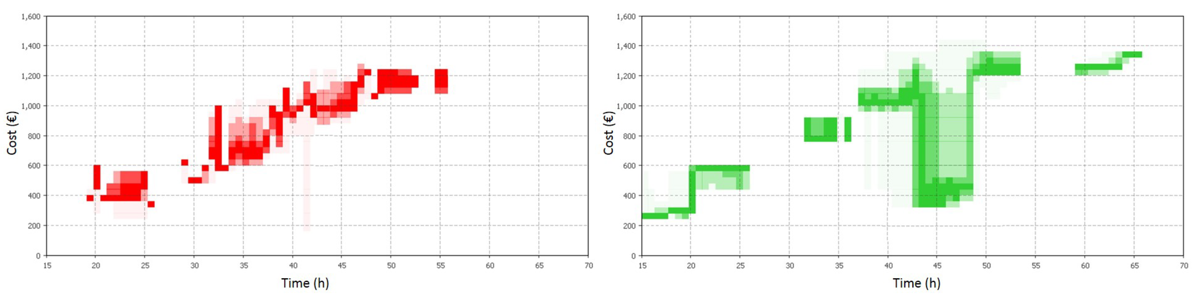
Disruption profile $\Psi$2: when comparing intermodal (red) and synchromodal (green) simulations under disruption profile 2 (Figure 8), the results do not yield any significant difference in terms of cost (p ≥ 0.05) and distance (p ≥ 0.05). However, the figure visually depicts some orders which had to cover longer distances and slightly higher costs. This development can be attributed to the pro-activeness of agents that seek other available terminals in the synchromodal case (green). Given the insignificant difference in cost and distance, the modes that carried the orders play a crucial role. With regard to modal share,

Table 4. Comparison of static intermodal (S3a) and dynamic synchromodal (S3b) measures after exposing simulation 2 (S2) to disruption profiles.

	${\mathit{\lambda }}_{\mathit{o}}$ (Days)	Shifted/Unimodal (%)	Distance Share (%) (Road/Iww/Rail)	Cost Share (%) (Road/Iww/Rail/Term)	CO2-eq Share (%) (Road/Iww/Rail)
Disruption profile $\Psi$2
S3a	${\lambda }_{o5}$	26.5/73.5	79.1/4.3/16.7	83.1/1.1/12.5/3.3	94.5/1.6/3.9
	${\lambda }_{o2}$	10.6/89.4	89.6/0/10.4	91.2/0/7.5/1.3	97.8/0/2.2
	Total ${\mathit{\lambda }}_{\mathit{o}\mathbf{5}}$	-	887,337 km	€734,331	1,529,276 kg
	Total ${\mathit{\lambda }}_{\mathit{o}\mathbf{2}}$	-	903,215 km	€772,031	1,704,625 kg
S3b	${\lambda }_{o5}$	39.5/60.5	85.7/12.9/1.4	90.5/3.3/1/5.2	95.1/4.6/0.3
	${\lambda }_{o2}$	6.7/93.3	99.7/0.1/0.3	99/0.01/0.2/0.8	99.9/0.01/0.1
	Total ${\mathit{\lambda }}_{\mathit{o}\mathbf{5}}$	-	857,749 km	€706,639	1,592,733 kg
	Total ${\mathit{\lambda }}_{\mathit{o}\mathbf{2}}$	-	886,490 km	€779,639	1,821,216 kg
Disruption Profile $\Psi$3
S3a	${\lambda }_{o5}$	26.5/73.5	79.1/4.3/16.7	83.1/1.1/12.5/3.3	94.5/1.6/3.9
	${\lambda }_{o2}$	9.3/90.7	90.1/0/9.9	91.7/0/7.2/1.1	97.9/0/2.1
	Total ${\mathit{\lambda }}_{\mathit{o}\mathbf{5}}$	-	887,337 km	€734,331	1,529,276 kg
	Total ${\mathit{\lambda }}_{\mathit{o}\mathbf{2}}$	-	901,077 km	€770,122	1,707,463 kg
S3b	${\lambda }_{o5}$	58.4/41.6	80.4/19.6/0	87.1/5.1/0/7.8	92.8/7.2/0
	${\lambda }_{o2}$	2/98	99.9/0.1/0	99.1/0.1/0/0.8	99.9/0.1/0
	Total ${\mathit{\lambda }}_{\mathit{o}\mathbf{5}}$	-	853,963 km	€686,079	1,524,217 kg
	Total ${\mathit{\lambda }}_{\mathit{o}\mathbf{2}}$	-	884,934 km	€776,378	1,821,727 kg

shows the share of shifted orders increased from 26.5% (S3a) to 39.5% (S3b) due to the ability of trucks to query iww terminals that are further away than the rail terminals chosen by static intermodal solutions. The share of iww distances supports this claim as it increased from 4.3% to 12.9%. It is important to notice is the higher share of terminal costs that changed from 3.3% to 5.2%. The increase was caused by the higher shifted order share where more handling is required, but also by the terminal size as larger terminals are avoided and other smaller terminals are chosen. As indicated in our input Table 1, medium terminals charge €60 per handling instead of €36. Hence, the cost does not improve significantly for the synchromodal setting as the higher handling costs deteriorate the potential cost improvement. As far as the lead-time is concerned (Figure 8, right), the pattern differs significantly (p ≤ 0.05). The most visual outliers are between 60 and 66 h which can be explained by the risk-avoiding approach of synchromodality choosing terminals further away and incurring delays be unnecessary detours. This aspect generates higher share of road from 79.1% to 85.7% at the expanse of rail that decreased from 16.7% to 1.4% indicating that not all orders shifted to iww (Table 4). A cost decrease is observed between 45 and 50 h for green synchromodal dots (Figure 8, right) where choosing barge services located closer to the order’s final destination yielded lower costs as compared to the red intermodal dots above them.

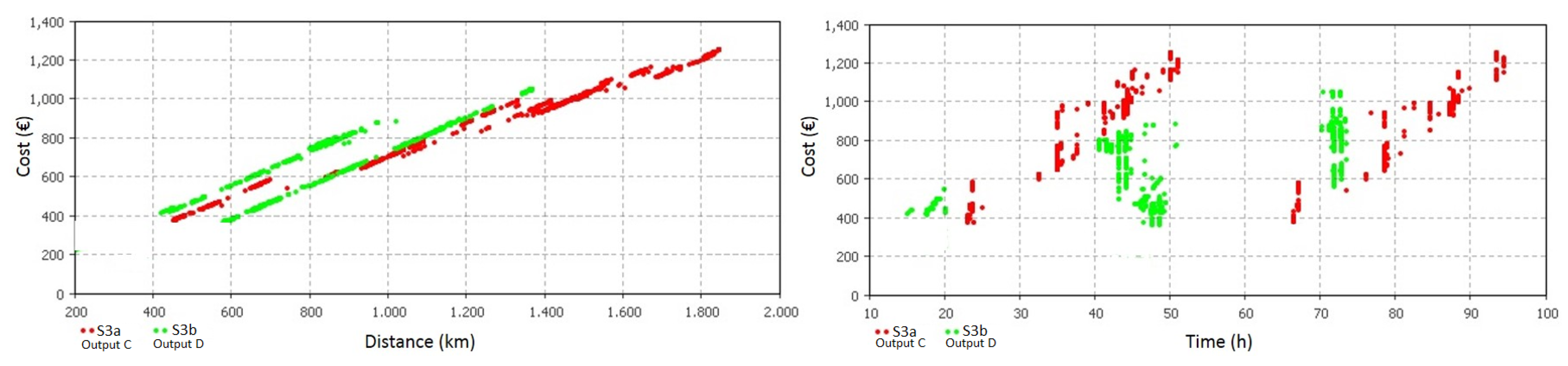
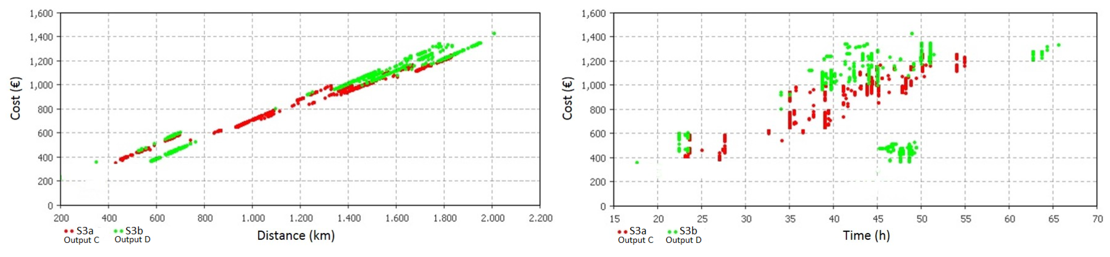
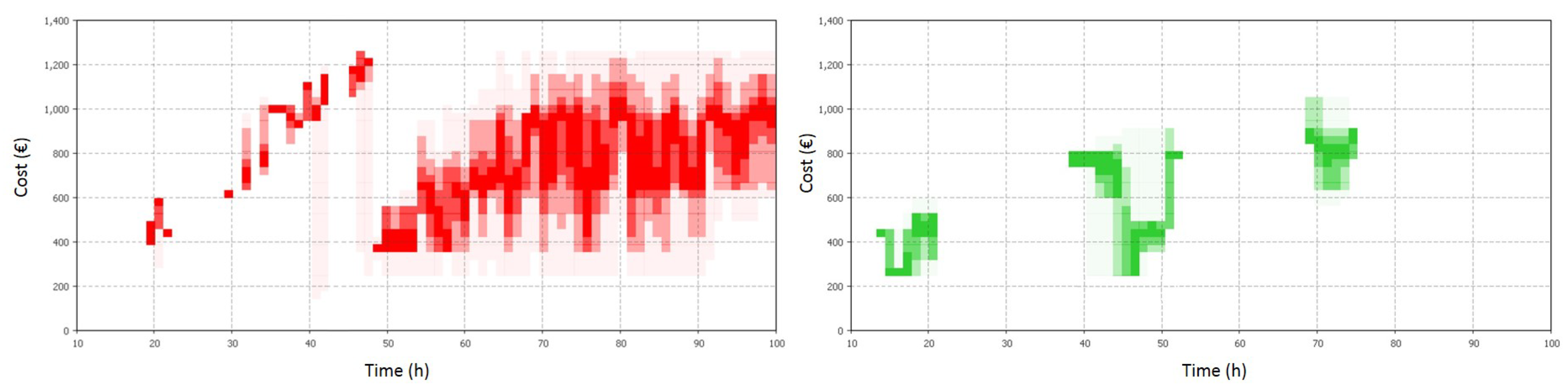
Disruption profile $\Psi$3: when applying disruption profile $\Psi$3 (Figure 9), the proactivness of synchromodality (green) yields significantly better performance in terms of distances (p ≤ 0.05), costs (p ≤ 0.05) and lead-times (p ≤ 0.05). This development was caused by the fact that all truck agents search iww solutions as the usage of rail is omitted. In this case the geo-spatial search goes beyond the 300 km radius, ignoring several rail terminal options that lay in between, until the nearest iww terminal is found. Given this setting, and the ${\lambda }_{o5}$ and cost thresholds $O_{s,dc}^c$ from S1, 54.8% of orders could be shifted from road-only transport. However, synchromodal flexibility is not always a better solution; while most of the green orders situated between 40–50 h outperform red orders in terms of cost and between 70–80 h in terms of time, it is observed that a small amount of red orders under €800 yielded relatively better cost and time results. This is an interesting development which implies that synchromodal solutions mitigate the effects of disruptions worse in terms of costs and lead-time for these particular orders; the intermodal static case (S3a) continued with deliveries once the disruption was over, unlike the synchromodal solution seeking case (S3b) that needed more time to deviate to another terminal. Handling cost may also play a role since smaller terminals charge more per handling than larger ones. In this particular case, it is more beneficial for some orders to wait at a disrupted path rather than search proactively for other solutions. Hence, the flexibility of synchromnodality may also yield more negative effects for a fraction of orders when compared to intermodal static options.

As far as emissions are concerned (Table 4), the synchromodal setting under disruption profile 2 generated 63,457 kg more as a result of a higher share of iww from 1.6 to 4.6% and a decrease in rail from 3.9 to 0.3%. The increase in road emission share caused by deviations is rather negligible. A reverse effect is observed under disruption profile 3 when the synchromodal solutions decrease emissions by 5059 kg. This effect is attributed to higher iww share (1.6 to 7.2%) in combination with lower road share (94.4 to 92.8%).

5. Discussion

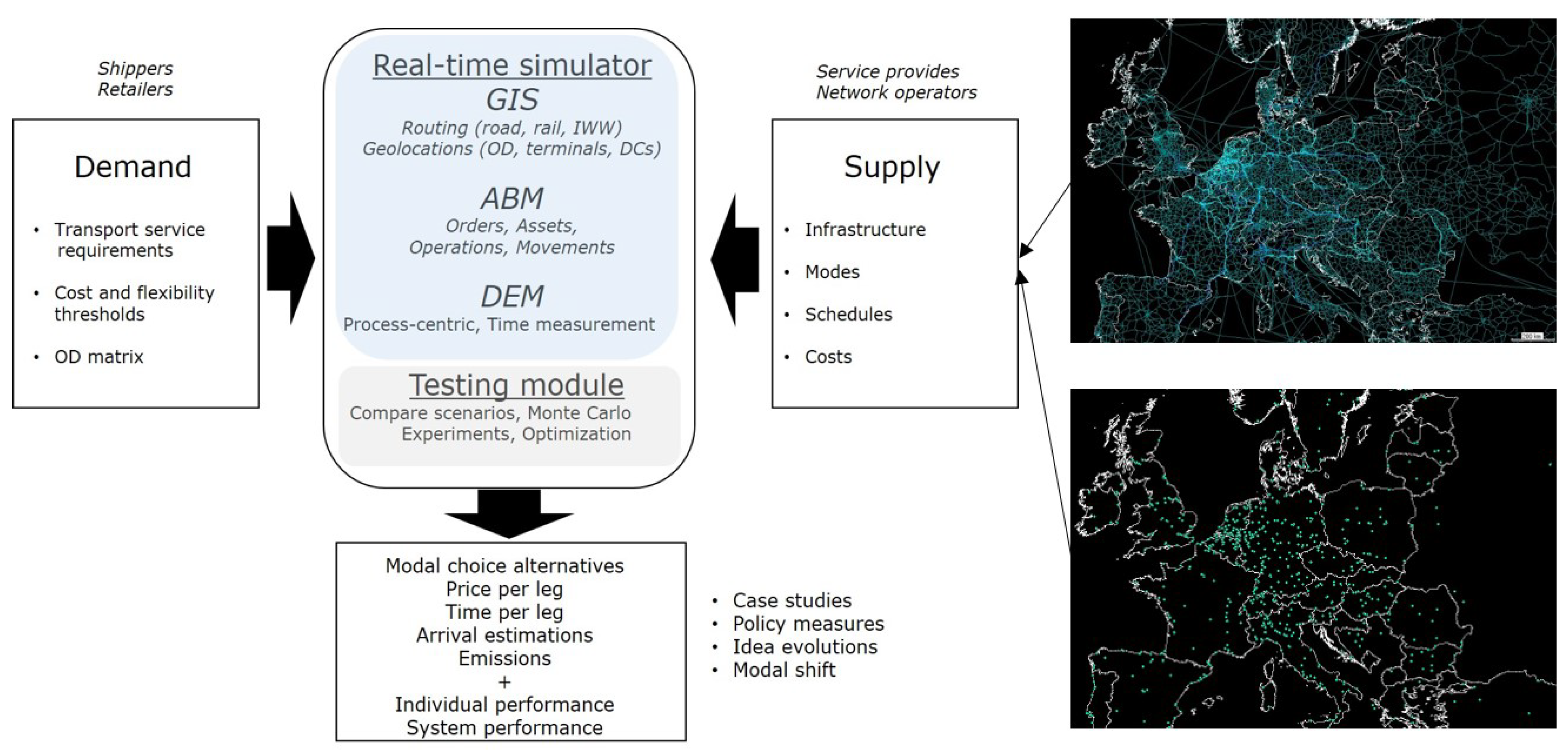
Managerial implications: the simulation experiments provide a range of alternatives and assessments which may also be of interest to other retailers who rely on truck-only transport. To answer our first research question (what is the modal shift potential of individual dispersed orders served by truck-only when imposing lead-time and cost thresholds?), the modal shift potential is 26.5% and may increase to 39.5% and 58.4% when allowing for synchromodal solutions. These solutions, however, rely on network openness and benevolence of other carriers to flexibly change modes at any time. Our work presents the benefits of having such an open network where orders may be transported by a different mode, depending on its availability in geographic space. The 26.5% shift potential can incur savings of €37,545 and 298,170 kg of emissions per year. These estimates change if stricter time windows are imposed. Such strict time windows concern around 10% of the orders in case of our retailer, and these urgencies are caused by miscalculations, frequently used products, unexpected peaks in demand etc. Given the rather attractive benefits in terms of cost and emissions, there is still a lack of intermodal service offer for the order locations with modal shift potential. The LSPs offer truck-only solutions due to the fact that a limited number of back-flows is present to fill a train or a barge for a return trip. As a matter of fact, the fragmented flows are currently not interesting for LSPs as they prefer full trains from one factory to another. Retailers cannot induce a modal shift on their own because they do not have the necessary volumes and power to carry the costs and experiments alone. It is thus necessary to gain insights and identify flows that would fill return trips. In this regard, transparency and information sharing is crucial. SYMBIT can be perceived as a platform that has the ability to simulate fragmented retail flows and assess what-if scenarios. The model exposes the potential for a modal shift of a company, but may also compute bundling scenarios with another company with similar backward flows. Without having critical stable mass however, the alternative of single-wagon-loads (SWL) could be explored. This might imply development of hybrid structures that allow for block train volumes being integrated with SWL business. A setting of this type could enable accessing stable base volumes that could also benefit from high return SWL of the retailer presented herein. In other words, existing train and barge services would have to be connected with local trucking companies to offer more reliable services by reinforcing each other. In terms of implementation, more case studies and European pilots are necessary to further strengthen the synchromodal idea. Furthermore, standardization at a European level is a crucial element due to diverse working cultures, different levels of digitalization and automation as well as willingness to share information among member states and companies.

Research implications: real-time simulations within GIS can be extremely powerful and accurate. Nonetheless, these are currently underexploited. Objects/agents have the ability to learn certain aspects of the model during execution; when parameters or the context change, the agents will try to find solutions that meet their objectives in realistic space and time. These spatial and temporal dimensions are not depicted by current synchromodal models, and those which do include GIS, make use of them for visual interpretation of results and ex-post analysis. Hence, GIS are currently never or rarely embodied in the simulation process itself.

As for our last research question (does synchromodal dynamic reconfiguration have any impact on the lead-time, cost and emissions compared to a, more static, intermodal setting?), our approach sheds light on the uncertainty regarding cost and time thresholds once intermodal solutions are exposed to disruptions. Disruptions and delays occur in reality which is why SYMBIT’s architecture is devised to reconfigure when exposed to perturbations. This is achieved by decentralized intelligence of each agent and its local possibilities facilitated by spatial and temporal awareness. As mentioned earlier, deliveries under disruption profile 1 are robust enough to small deviations. With regard to disruption profile 2, shifting modes dynamically is not always required because the extra deviations and unnecessary pro-activeness decrease the potential emission and time savings. Therefore the disruption severity needs to be considered when thinking about proactive solutions and whether these proactive solutions are worth the deviations and switching in terms of KPIs. Despite visual observations, the differences under profile 2 are not statistically significant. However, synchromodality does present a significant improvement when dealing with longer and more severe disruptions. In this regard, more advanced algorithms would be needed to answer each agent’s question: should I stay or should I go? This is a very challenging task as the disruption length uncertainty is not always known in reality, which presents a major challenge. New sensor technologies and techniques that can collect and integrate real-time information will be imperative to determine the disruption severity, its length and spatial occurrence in order to reduce uncertainties depicted by probability distribution functions. The earlier mentioned network openness can be achieved through IoT technologies and geo-spatial coverage, by 5G network for instance, in order to reach out to assets by facilitating information exchange, remote-control and automation.

6. Conclusions

This paper assesses the modal shift potential of hundreds of real-world scattered orders. We provide evidence that intermodal solutions can be efficient in terms of cost and time. Furthermore, the potential orders could yield significant cost savings of nearly 5% on a yearly basis and mitigate the overall environmental impact by 16%. These benefits ameliorate when applying flexible and dynamic synchromodal solutions. However, the benefits diminish for most of the orders when imposing two-day time windows which is why better planning and demand forecasting are imperative to avoid such developments. From a methodological perspective, our approach offers the ability to simulate information availability/exchange that is linked to consequent reactive agent behaviour induced by it. This ability of SYMBIT is tested by exposing static solutions to disruptions where individual agents reconfigure based on their position in space and time. Knowing the state of the transport system and its evolution allows for more accurate and efficient policy rules to mitigate the undesired effects of the system and its sub-parts. Synchromodality does offer more alternatives, but these alternatives should be assessed carefully as the performance may not always be more beneficial than the more static intermodal solutions. As far as disruption management is concerned, future research could focus on more severe disruptions such as the known occurrence of a sink hole in rail tracks within the Rhine–Alpine corridor. Our agent reconfiguration may contribute to testing the resilience of possible disruption management schemes to tackle similar events in the future. Future work could also include dynamically changing speed profiles of agents to account for peak hours in specific geographical regions. The horizontal collaboration dimension and bundling scenarios with revenue management should be considered as well, once another company’s similar flows are exposed.