Abstract
Any change in the geometric configuration of the existing road affects other dependent elements such as travel time, fuel consumption, and existing pavement. This paper quantifies these effects and finds an optimum geometric configuration. Three separate models are developed in this research: (1) the travel time model which predicts vehicles flow speed on the specified geometric condition, traffic composure, and evaluates the imposed costs to the road users; (2) the fuel consumption model, which estimates needed propulsive force and anticipated fuel for vehicles passing through the road; and (3) the pavement rehabilitation cost model considering two main constraints of existing pavement condition and project line elevation. The developed pavement rehabilitation model proposes the best solution for pavement rehabilitation practice and computes associated costs. Particle Swarm Optimization (PSO) is used to find the optimum solution in a minimization problem search space. The proposed model is applied to a real-world case study. Results show that there is an extremely less tendency for change, even with the existence of adverse geometric conditions, when there is a relatively good pavement condition. In the case of deteriorated pavement conditions, economic justification for geometric modification is required.
1. Introduction
1.1. Problem Statement
Maintenance, rehabilitation, and modification of existing roads impose remarkable human and financial resources to road owners and road users. There is a need for robust management to sustain the appropriate condition of the road and minimize the rehabilitation costs. Road rehabilitation mostly divides into two different categories: (1) the geometric modification of the road which would be conducted in a certain condition such as accident vulnerability prevention, traffic flow enhancement, access adjustment, etc., and (2) pavement rehabilitation which would be conducted on a regular basis and depends on the pavement condition. It may be done all over the road pavement, such as a complementary overlay, which mostly applies in the second half of the pavement designed life and may apply in certain segments of the pavement that locally suffer from deteriorated conditions. Any change in the geometric design of an existing roadway causes a high capital investment in the construction because of excavation, embankment, pavement construction, and other existing constraints, as well as travel time and fuel consumption. The sensitivity of these parameters and their impacts on overall cost are different in nature.
This paper aims to develop a framework for geometric changes of an existing road, measures the impact on dependent parameters, and optimizes variation by establishing a model for geometric modification of vertical roadway alignment. Since the geometric changes of the existing roadway affect the traffic flow and fuel consumption (user costs), two separate models need to be established to calculate the associated costs. We therefore use the Particle Swarm Optimization (PSO) algorithm in combination with the developed pavement rehabilitation cost model; the best solution is achieved within a minimization problem.
In the following sections, the geometric components of the vertical alignment are described. After reviewing the previous research background of road alignment optimization models, the developed models for cost estimation (travel time cost, fuel consumption cost, and pavement rehabilitation cost) are discussed in detail. With the introduction of the optimization model, all the required information is gathered in the PSO framework to propose an optimum solution. A real-world case study is conducted to evaluate the palpability of this model and the results are discussed.
1.2. Research Background
The first generations of road alignment optimization models have been developed in the late 60s [1,2]. With advancement in computer process capabilities in the 70s, this model progressed accordingly [3,4,5] and, nowadays, there is a rich bibliographic background. There are numerous models which can be considered in three main categories: (1) optimization methods; (2) dimension and number of optimization objectives; and (3) cost functions and level of detail with which these models have been used. There is a wide range of optimization methods for road alignment model that can be categorized into classic and metaheuristic methods. Classic methods include mixed integer linear programming, dynamic programming [6], mixed integer linear programming [7,8], etc. Metaheuristic methods including Genetic Algorithm (GA) [9] and swarm intelligent-based methods (e.g., PSO [10,11]). There are some advanced methods which use the Combination of GA and Geographical Information System (GIS). This pair of GIS and GA models are known as Highway Alignment Optimization (HAO) models [12,13,14,15,16].
If there is more than one dependent variable in optimization, all variables convert into one mutual dependent value which is usually cost and the problem is solved as a single-objective problem. In some cases, bi-objective [17] and multi-objective [18] frameworks are proposed which provide a wider selection range for decision makers. With the evolution of models, more complicated and detailed cost functions and various road conditions embed into models to cover different settings and enhance the flexibility and versatility of models. Different road circumstances, such as regional route locations [5], forest roads [19], permafrost regions [20], ecologically sensitive area [21], and environmental constraints [22], were investigated with their specific design characteristics. Several cost functions for highway alignment optimization models were proposed by Jong and Schonfeld [13]. Various objectives, such as minimization of fuel consumption and improving safety [23], sight distance [24], roadside slope and block regions [7], and optimization in a pre-allocated corridor with more accuracy [25], were studied in recent researches. Table 1 shows the summary of relevant researches over the past four years and their innovations.

Table 1.
Recent highway alignment optimization models in the past four years.
Although the optimization models have been propagated in the last decades, the rehabilitation and reconstruction models are in their infancy, except for some recent models [26]. Most of the recent researches contributed to cover diverse conditions and provide a solution for each one. Developed countries are currently dealing with large size existing roadway networks and high maintenance cost of these roadways, which highlights the necessity for expanding the research on rehabilitation and modification of existing roads. The main contribution of this research is focused on the horizon of alignment optimization with a rehabilitation model of the existing road by proposing a framework for pavement rehabilitation design.
2. Methods
An overview of the proposed method is shown in Figure 1. The cost models used in the proposed method in this research including fuel consumption cost related to the travel time of passing vehicles and pavement rehabilitation accompanied costs are discussed in detail.
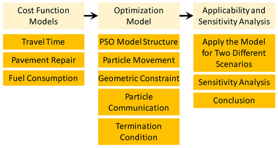
Figure 1.
An overview of the proposed method.
2.1. Cost Components
2.1.1. Fuel Consumption Estimation
Fuel consumption of a vehicle is sensitive to grades in vertical alignment and directly depends on road geometric design particularly resisting forces applied to the vehicle as shown in Figure 2. These forces are grade resistance, rolling resistance, the internal resistance of vehicle, and air resistance. Vehicle internal resistance can be neglected in the model because it is relatively constant in different geometric conditions for a single vehicle.
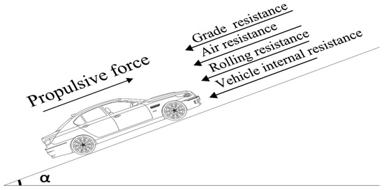
Figure 2.
The propulsive force applied to move the vehicle on a gradient.
The fuel consumption model, which is deployed in this research, considers three main forces, including the grade resistance, the internal resistance of the vehicle, and air resistance. For a vehicle, this force is simply calculated as
where W is the total required propulsive force, is the gravity resistance force, is rolling resistance force of moving vehicle, is air resistance force, m is mass of vehicle, is gravitational acceleration, is rolling resistance coefficient, is grade angle, Af is a front area of the vehicle, is the air density of the vehicle, is the drag coefficient, and V is the vehicle speed.
There exist five categories of car—Recreational Vehicle (RV), bus, empty truck, and loaded truck—that are defined for different vehicle weights and characteristics. In the proposed model, it is also assumed that the vehicle moves with constant cruise speed. In order to neutralize friction and gravity forces, there is a need for a compensating force to maintain the constant speed. Figure 3 shows the change of needed propulsive force in a route with a sample longitudinal profile for five different vehicle types. The model shows that for heavier vehicles in steep upward slopes the needed propulsive force increases sharply (see the propulsive force for loaded truck between 2 + 600 and 2 + 700). In contrast, in steep downward slopes, a need for braking action exists for heavy vehicles. The red dotted line shows the minimum average grade which imposes minimum fuel consumption cost.
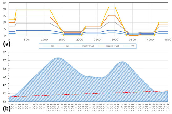
Figure 3.
Change of propulsive force for different vehicles (a) in different geometric designs (b) of road.
Equation (2) is used to quantify the needed fuel for movement of vehicles on designed geometric composure of road (VF): this is the estimate of the equivalent fuel to provide the needed propulsive force (W) using fuel consumption rate (rf is in Liter/Joule).
In order to calculate the extra fuel consumption due to the geometric configuration of the road, the fuel consumption in the base condition needs to be subtracted from the total consumption. Fuel consumption in base condition is defined as an amount of fuel consumption from starting point to the endpoint passing a straight line as shown in the red-dashed line in Figure 3. The extra fuel consumption is calculated as Equation (3):
where Cf,model is the extra fuel consumption cost due to geometric change used in the model, Cf,new is fuel consumption cost of the new condition of the road, and Cf,basic is fuel consumption cost in the base condition.
2.1.2. Travel Time Cost
In the Highway Capacity Manual (HCM), a comprehensive procedure to evaluate traffic speed consequent travel time has been presented. This is discussed in the second volume of HCM (uninterrupted flow) in Chapter 11 (basic freeway segments). This method has been adapted for travel time computations. In the proposed model, it is assumed that (1) the studied freeway segments has three lanes with 3.65 m width for each lane and 1.8 m shoulder at right side with PHF (Peak Hour Factor) = 0.85, FFS (Free Flow Speed) = 110 km/h, and a flow rate (in prevail condition) of 1600 pc/h/lane; (2) there is no on-ramps/off-ramps or merge/diverge zone; and (3) that the same conditions apply to all proposed project lines in the base conditions of the studied segments, including good weather and visibility, no accidents, no work zone activity, and pavement deterioration does not affect the traffic stream.
Since the freeway is in service and the traffic data is available, the values of traffic parameters are determined based on an on-site survey of the existing freeway. There are multiple steps required in order to calculate the travel time for freeway segments as follows.
- Vehicle demand volume and speeds
In the first step, demand volume should be converted from prevailing condition (which is evaluated on site) into the equivalent base condition to accommodate variations in PHF, the number of lanes, the grade value and grade changes, traffic configuration, and the driver’s familiarity of the roadway. Equation (4) quantifies the effect of changing each of these factors on demand flow rate:
where vp is the demand flow rate under equivalent base condition (pc/h/ln); V is demand volume under prevailing conditions (veh/h), which is estimated on site; PHF is Peak-Hour Factor; N is the number of lanes in analysis direction; fHV is an adjustment factor for heavy vehicles (bus, truck, and recreational vehicles) when there is a critical condition of slope and length of slope for vertical alignment of the road; and fp is an adjustment factor to consider the effects of unfamiliar drivers. The commuter vehicles have more familiarity and less negative effect on the traffic stream. The recreational vehicles also have less familiarity and more negative effects on the traffic stream. This number ranges between 0.85 (for completely unfamiliar driver population) and 1 (for absolutely familiar drivers).
fHV is derived from Equation (5), where PT and Et are the proportion of trucks in traffic stream and equivalent factor for trucks, respectively, and PR and ER are the proportion and equivalent factor for recreational vehicles, respectively. The vehicle equivalent factor has different values for the different grade conditions of roadways, including general terrain, specific upgrades, and downgrades. For moderate and flat slopes, the equivalent values of trucks, buses, and recreational vehicles can be derived from Table 2.
Table 2.
Passenger car equivalent by type of terrain.
When the tangent’s grades and its length intensify, the speed reduction of heavy vehicles increases and, consequently, impacts the other vehicles on the highway. This effect depends on grade value and grade length percentage of heavy vehicles on the roadway. When the tangent’s grades and its length are intensified, the speed of grades between 2% and 3%, and longer than 0.5 miles or 3% and longer than 0.25 mile, would be considered as ‘special upgrades’.
The developed traffic model calculates this value based on each of the segment slope’s characteristics and measures the effect of the geometric change on vehicle speed. In upgrades, the speed reduction of heavy vehicles occurs more rapidly and it takes longer to recover the speed. This speed reduction affects the speed of the following vehicles and consequently the flow of vehicles. In longer and sharper slopes this effect intensifies. In contrast with upgrades, the speed reduction of heavy vehicles is due to the use of low gears to avoid speeding up for better control of the vehicles on downgrades. This affects the speed of other following vehicles.
- Speed based on existing condition
After determining vp based on adjusted existing roadway configurations, the average speed of passing vehicles is calculated. This equation proposed in HCM [28] is based on FFS and flow rates of passing vehicles. For FFS = 110 km/h:
where VAdjusted is adjusted passing vehicles average speed based on local traffic and the geometric and roadway configuration. This value is needed to calculate the travel time of passing vehicles. vp is calculated based on the existing condition of traffic and roadway configuration.
- Quantification of travel time cost
After determining the average speed of traveling vehicles, the overall time of travel between the starting point and endpoint can be calculated by dividing this distance by the average speed of traveling vehicles. The average occupancy rate of each type of vehicles is determined based on the on-site survey study. The value of time for each type of vehicle can be calculated using Equation (7):
where Ctt is the cost of travel time for all vehicles in all design period days; is total days in the design period; is a number of vehicle types; is Annual Average Daily Traffic which passes in all lanes; is Average Travel Speed; is average occupancy of vehicle type; is a percentage of vehicle type (ith) in all vehicles; is hourly wage rate; and is the value of time derived from Table 3.
Table 3.
The value of time for the passengers of different vehicles.
- Extra travel time cost due to geometric changes
To calculate travel time due to the road geometric configuration and specify the exclusive effects of geometric changes on travel time, it is necessary to separate it from the base condition of the roadway. The base condition is defined to calculate the minimum travel time cost between starting and endpoint of the roadway. Any geometric change may increase this cost. The base condition is defined as a simplest geometric composure in longitudinal profile which is a straight line with a constant slope as shown the red dashed line in Figure 3. The exclusive geometric cost for travel time in the model can be calculated as
where Ctt,new is the cost of the entire travel time of the new configuration of geometric design and Ctt,basic is the calculated travel time in the base geometric configuration of the roadway longitudinal profile.
2.1.3. Pavement Rehabilitation Cost
This research proposes a new model for the existing pavement structure. Therefore, selecting and estimating construction means and methods are more complicated in comparison with the new construction. Pavement reconstruction design depends on two main factors: (1) the difference between a new project line (PL) and existing ground (GL) and (2) existing pavement condition. Both of these two factors are important to choose a rehabilitation strategy. Figure 4 schematically shows the layers of existing pavement and its condition over new PL. The position of different PLs in comparison with existing pavement layers is shown in this figure.
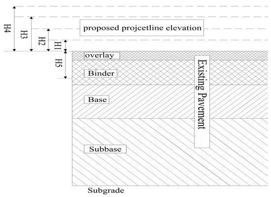
Figure 4.
New project line (PL) and existing ground (GL) differences.
There are different conditions based on existing pavement elevation and new project line elevation:
- In general rehabilitation practice, a complimentary layer applies on the existing pavement to enhance pavement efficacy for applied loads (H1 = minimum complimentary overlay layer’s depth).
- When the difference between Pl and GL increases and project line elevation exceeds H1 (H1 ≤ ΔH < H2) an overlay material would be used to cover this difference.
- With a greater increase in ΔH (H2 ≤ ΔH < H3) and exceeding the summation of the minimum allowable thickness of binder and minimum allowable thickness of the overlay layer, (ΔH > Hminoverlay + Hminbinder), a cheaper (in comparison with overlay) layer of binder would be used below the overlay layer.
- With increasing ΔH (H3 ≤ ΔH < H4), filling this depth with asphalt concrete makes the rehabilitation cost increase sharply. Another solution is to remove the existing pavement, applying an additional adjustment base (cheaper material) layer and then reconstructing the other top layers of the pavement. In other words, instead of filling the gap between PL and GL with an expensive layer of asphalt concrete, the cheaper layer of the base would fill this gap.
- If the difference increases more (ΔH > H4), the full depth reclamation of pavement, embankment to reach decent elevation and reconstruction of all pavement applies.
Damages occur in the pavement structure when it is exposed to loads of passing vehicles. Pavement damages may occur in any layer of pavement (overlay, binder, base, and subbase or subgrade). A conceptual “modified ground line” is introduced based on the severity and depth of deteriorations to estimate rehabilitation cost of damaged parts and associate it with the geometric terms. This modified ground line (GL*) shows the top layer of pavement where lower layers do not suffer from major damage. The modified ground level concept (GL*) is illustrated in Figure 5 and GL-GL* shows the deteriorated depth of pavement.
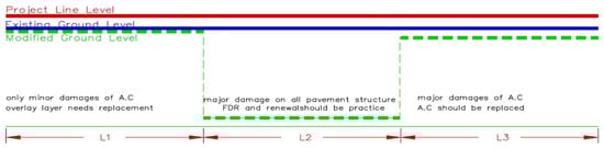
Figure 5.
Different conditions of the longitudinal profile for PL, GL, and GL* (vertically exaggerated).
As shown in Figure 5, there are three different conditions of existing pavement condition. In the first segment, the pavement has a good condition so it has a minor difference between GL and GL*. These minor damages are only in the overlay layer and can be repaired with milling and adding an overlay layer. In the second segment (L2), there is damage to the lower layers of pavement. The subgrade may need to be replaced or stabilized in this section. Hence, it is essential to reclaiming the existing pavement in full depth. Subgrade rehabilitation and then new construction of pavement should be executed. In the third segment, the asphalt concrete including overlay and binder has major deteriorations that it has to be replaced with new asphalt concrete. In this case, the difference between GL and GL* is equal to asphalt concrete pavement thickness. The modified ground line (GL*) concept is a practical tool for understanding the existing pavement conditions and deteriorated depth. It converts the pavement condition into a geometric pattern to consider in the geometric design of the longitudinal profile. The pattern in Table 4 is used to select proper treatment to quantify the pavement rehabilitation practice. The accompanied cost for each of these practice types calculated based on the unit cost [29].
Table 4.
Practice type selection and its practical details based on different states of PL, GL, and GL*.
There is a rehabilitation cost for treatment of existing pavement. This cost is divided into two main categories: (1) the existing pavement rehabilitation practice, which includes all costs related to repair of the pavement (Crehab), and (2) complementary overlay on the entire pavement (Coverlay). These costs are geometric-independent. Therefore, the geometric-dependent cost can be achieved from
where Cp,model is the geometric cost of pavement rehabilitation practice and Cp,new is the total cost of pavement repair.
2.2. Geometric Components
2.2.1. Geometric Composure of Vertical Alignment
The main components of a vertical alignment in the geometric configuration are grades (upgrade and downgrade) and curves (sag and crest). These curves, based on applicability, have circular or parabolic equations. For roadways, the parabolic curve is used with an equivalent vertical axis centered on the vertical point of intersection. If the outward tangent of the curve has a greater value than the inward grade, the curve is concave (sag); otherwise, it is considered a convex (crest) curve. Figure 6 shows the configuration of the parabolic longitudinal curve.
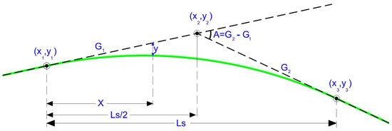
Figure 6.
Parameters of tangents and parabolic curve in longitudinal profile.
The two intersecting tangents have a linear equation in the first and second tangents, as shown in Equations (10) and (11):
The curve has a parabolic equation in form of
In which a, b, and c are
2.2.2. Geometric Restrictions of Vertical Alignment Components
- Grades
There are maximum and minimum grade restrictions for highway longitudinal alignment. Absolute maximum restrictions have been implied to avoid excessive deceleration of heavy vehicles. The minimum grade also assures better drainage of the roadway. The desirable minimum grade for proper drainage is 0.20 percent. On the start and endpoints of the project, the slope and elevation of the new project line should be compatible with existing road alignment. This condition is considered in the configuration of every project lines.
- Curves
Minimum stopping sight distance is a design control for vertical curve length. In vertical curves, this distance depends on slope change (A) and the rate of vertical curvature (K). K represents the needed horizontal distance in meters to make a one percent change in gradient. The K value varies in different types of curves (sag vs. crest) and design speeds. The absolute value of the change in gradient (g) also has a restriction for sag and crest vertical curves:
where g is the absolute algebraic difference in gradient (%), L is the length of the vertical curve (m), and S is sight distance (m). For divided multilane highways, if there is no opposing traffic stream, the minimum length for passing maneuver will not be an applicable criterion.
2.2.3. Applying Evolutionary Change for Each Intersecting Points of Tangents (IPS)
In the optimization procedure, the change of IPs leads to the evolution of the solution. This change should be compatible with design criteria satisfies all technical requirements for longitudinal direction. In the first step, the affected length of each IP should be determined. For each presumed IP change, the inward and outward tangents and curve length of that IP would change. Furthermore, variation in the slope of these tangents affects the delta angle (A) of the previous and next IPs and, consequently, it changes the curves of two adjacent IPs. Figure 7 shows the affected length of changing one IP.
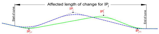
Figure 7.
Affected length of longitudinal profile due to change of IP location.
For every change in each IP, there are three changing components: change in km of each IP (x), elevation of each IP (y), and length of curve Ls.
- “x” variation restrictions
In the optimization procedure, the “x” component moves in the solution space and there is a restriction for each IP’s x coordinate movement. A changing domain for x is defined as the mid-distance between two adjacent IPs .
- “y” variation restrictions
Assuming x position, the change of y should be bounded. There are several components which restrict the y boundary. It comprised of maximum and minimum allowable slopes for inward and outward tangents, minimum curve length for changing IP, and its adjacent curves. Some subjective changes due to the change in IP arise in two neighboring curves. In order to justify this curve for the new condition, it would change proportional to the change of angle difference (A) for these IPs.
As is shown in Figure 7, the change of IPj affects the adjacent tangents gradient, i.e., IPj−1 and IPj+1 (and therefore curve length). To adopt this change, the new curve length (Ls2) would be
where are the length of the curve, angular change, and curve length coefficient before the change of IP, respectively, and are the length of the curve, angular change, and the curve length coefficient after a change of IP, respectively.
- ” Ls” variation restrictions
As previously mentioned (in Equations (16) and (17)), the minimum curve length should satisfy the sight distance requirements. Therefore, the minimum curve length is based on sight distance and corresponding equations. The maximum length of the curve for ‘ith’ IP is
2.3. Optimization Method—Particle Swarm Optimization (PSO)
2.3.1. General Formulations
Particle Swarm Optimization (PSO) is a population-based stochastic optimization method inspired by the social behavior of agents [30]. This system is initiated with a population of random solutions and searches for optima by updating generations. In PSO, every single solution is a particle in the search space. All of the particles have fitness values that are evaluated by the fitness function. Every particle has a velocity which orients the moving of the particles. The particles move in the problem space by following the current optimum particles.
This method is initialized with a group of random particles and then searches for optima based on updating these particles in every iteration. Each particle is updated by the two best values including Personal Best (Pb) and Global best (Gb). Pb is the optimized value which one particle achieved and Gb is the optimized value achieved between all particles. With these two values, the particles move in solution space. The movement pattern is defined with
where is the velocity of ith particle in kth iteration; r1 and r2 are random numbers generated uniformly between 0 and 1; c1 is the coefficient of personal best for one particle and c2 is the global best coefficient; w is the inertia factor of particle movement; and is the current solution of ith particle. The first term of this equation represents the effect of inertia of particle, the second term is related to the effect of previous particle’s experiences, and the third term represents social communication between all particle experiences.
In this research, the optimum finding problem defines as minimization of all costs due to the change of vertical alignment subjected to geometric constraints. A four-step procedure is defined to solve this minimization problem with the PSO algorithm: (1) Define the initial condition of the PSO model; (2) create random solutions by number of particles and find the global best and the personal best; (3) PSO optimization main loop; and (4) the termination condition. In the following subsections this process is described in more detail.
2.3.2. Initial Condition of PSO Model
In this step, the optimization problem has been defined as a minimization problem:
where Ct, Cf, and Cp are the costs of travel time, fuel consumption, and pavement repair of the proposed vertical alignment, respectively.
To construct a PSO framework, a solution space and solution matrix should be defined to resemble the vertical alignment characteristics. This matrix has a 3 × N dimension, which N is the number of IPs on the vertical curve. Each IP has a kilometer value (x), elevation value (y), and curve length (Ls). The number of IPs is the same as an existing condition. Figure 8 shows the matrix resemblance of geometric configuration for vertical alignment of the highway.
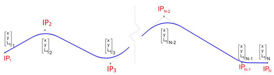
Figure 8.
Matrix modeling of vertical alignment.
In the next step, a number of particles and iterations should be defined. The number of particles mostly depends on the nature of optimization problems such as search space, number of variables, and the nature of the movement of particles. The number of particles is basically determined based on a trial-and-error method and usually considers problem dimensionality three or four times. The number of iterations is also determined by the quality of answers.
Then, the PSO coefficients of movement inertia coefficient (w), the personal experience related coefficient (c1), and social coefficient (c2) are determined. These coefficients have been studied by Clerc and Kennedy [31] using a theoretical approach to make the algorithm work efficiently by the following equations.
where is the constriction coefficient. The other parameters are the same as Equation (21). The most efficient value for is [31]:
where and the values of constriction coefficients c1, and c2:
These coefficients describe the particle’s movement and communication pattern. When these coefficients do not define precisely, the optimization procedure will not expand in search space and converge properly and as a result, the final answer will not be unreliable. If the global best coefficient is set to higher than the standard values, then exploration in the search space will not be adequately achieved and the final answer may not be an optimum solution as shown in Figure 9a. In contrast, if the personal best coefficient sets to inappropriate higher values, the vulnerability of getting stuck in local optima increases as shown in Figure 9b. This is due to the lack of movement toward the best solution and because each particle mostly sticks to improve its personal answer and communication and experiences exchange with other particles weakens. To tune the communication between particles while sticking to particle experiences, this coefficient should be defined properly (Figure 9c).
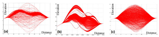
Figure 9.
Proposed solutions for different search space of particles when (a) CGB >> CPB, (b) CGB << CPB, and (c) the appropriate condition.
2.3.3. Create Random Solution by Number of Particles
After finding the PSO framework, the random solutions (particles) are developed by applying geometric restrictions of vertical alignment. The proposed model was developed in MATLAB. The random solution particle (i) is a 3 × N matrix, which N is the number of IPs in vertical alignment.
In the next step, all the particles are evaluated with different functions to calculate travel time, fuel consumption, and pavement construction practice costs, separately. The total cost for each particle is then obtained. Since there is no previous experience for any of the particles, this value is assigned as a personal best for each particle. The minimum value among all particles is reflected as the global best cost (Gb.cost) and its geometric configuration is used as the global best position (Gb.position) in the evolution procedure. In this step, the PSO procedure is defined for n particles and m iterations as the n × m matrix. The first column is filled with values and other columns are remained empty and will be filled during PSO evolutionary main loop.
2.3.4. PSO Main Loop
The developed matrix in the previous section is completed in cyclic iterations. In each iteration, Gb among all particles and the Pb of each particle should be updated and, accordingly, the movement equation for each particle changes during the evolution of solutions. Figure 10 shows the optimization procedure.
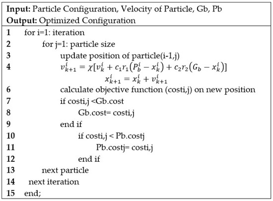
Figure 10.
The pseudo code of the main Particle Swarm Optimization (PSO) loop.
There are several methods to terminate the iteration of particles based on the problem condition. The important factor is to ensure the achievement of the mature answer. In this model, the maximum number of iterations without improvement of the objective function which is the total cost is used as the termination condition.
3. Data Collection and Setup
A real-world case study was conducted to evaluate and validate the proposed model in this research. The case study is a one-way three-lane highway with 4 + 500 m length. The optimum geometric design of highway under two different conditions is studied: (1) actual existing pavement in good condition with some local defects and (2) the hypothesized condition with the same geometric configuration as the first case but with assumed deteriorated pavement in some segments of the road. In other words, between stations of (0 + 185) to (2 + 105) all pavement layers are considered as deteriorated layers. All other geometric and pavement conditions stay the same. Figure 11 shows the longitudinal profile and deteriorated depth of the existing pavement for both cases. The basic parameters used in the case study are listed in Table 5.
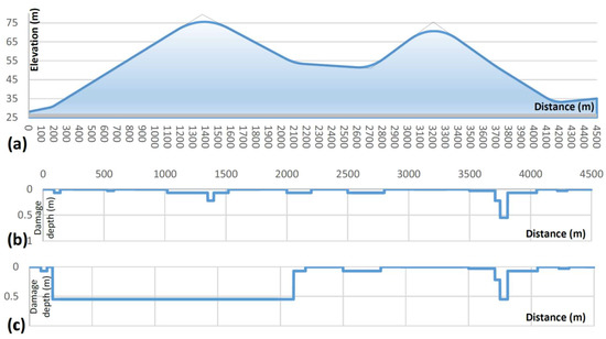
Figure 11.
Vertical alignment of existing road (a) and pavement deteriorated depth in the first (b) and second (c) case studies.
Table 5.
Case study assumptions.
4. Results and Discussions
For both scenarios of the case study, the cost evaluation models for travel time, fuel consumption, and pavement construction were applied. These costs were optimized using the proposed PSO-based optimization model to achieve the best solution. In both cases, the results of the cost function for fuel consumption are mostly the same while there are some major differences in travel time cost and pavement rehabilitation cost.
The optimized solution in the first condition lies on the existing ground. Since there is a relatively good condition for most of the segments of the pavement, changing the project line imposes a high cost on road rehabilitation practice and, consequently, this change was limited. In contrast, in the second case, where there is a deteriorated pavement condition between stations (0 + 185) to (2 + 105), this high sensitivity of change did not exist. Hence, there is a tendency of alteration to reduce the slope and positive effects on fuel consumption cost and travel time cost of the road. Figure 12 shows a minor reduction in fuel consumption but a major change in Free Flow Speed of vehicles between (0 + 185) to (2 + 105), as shown in Figure 13.
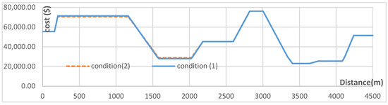
Figure 12.
Fuel consumption cost for both conditions.
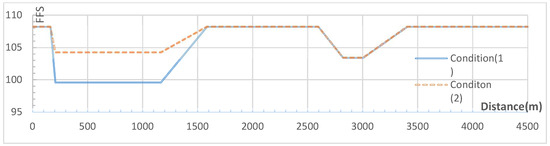
Figure 13.
Free flow speed (FFS).
To achieve a better understanding of the variation trend for cost variables, a sensitivity analysis was conducted for these two conditions. These cases, which have been previously introduced, have been shown in Figure 14 with (1) for the first and (2) for the second case study. The sensitivity analysis performed with changing the geometric configuration of the longitudinal profile with altering one IP’s elevation. The third IP, which is located at (1 + 375) km of the existing roadway, was moved vertically between (−5, 5) m with 1 cm increment. In both cases, the pavement conditions have two different pavement conditions of good and deteriorated. Figure 15 shows the trend of change in the variables. Due to the same geometric condition, the function for fuel cost and travel time cost is the same in both conditions, but there are two pavement cost functions. The total cost is also shown for both conditions. The cost functions used in the proposed model are the costs depend on the geometric changes of the roadway.
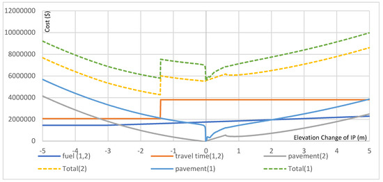
Figure 14.
Sensitivity analysis of cost functions.
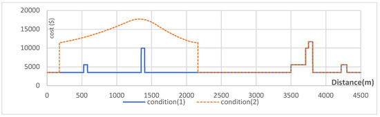
Figure 15.
Pavement rehabilitation cost.
The results show that in the good pavement condition there is a high sensitivity even in minor changes. This is because of changes in an expensive layer of asphalt. When the project line lies below the existing pavement, the compulsory deterioration of existing pavement imposes a high cost into reconstruction practice. Also, as shown in Figure 14, there is a low sensitivity to change of geometric configuration when there is a poor pavement condition. Which in this case, other factors would be dominant and geometric change would have an economic justification.
There are some limitations on developed cost models, especially on fuel consumption and construction cost models. In fuel consumption model, all passing traffic has been categorized into five vehicle types. This causes some approximation into the model. Adding more categories, results in more accurate modeling.
For simplification of model on evaluation of existing pavement condition, in each section, all cross-sections have been considered with the same pavement deterioration. When the number of lanes increases, this would increase the model’s cost assessment accuracy.
As discussed in the literature review, a new generation of optimization methods mostly applies to extend new conditions of the road into models. This research addressed the vertical road alignment optimization of existing separated multilane highways. Considering other aspects and conditions of this paper also would be studied in future works. The cost functions used in this study are applied to divided multilane rural highways. Other types of roads have different inherent characteristics, especially in traffic and safety concepts and would be more explored in future studies. There are also other types of pavements (such as concrete pavements, gravel, and even unpaved roads) which would be extended to this model. Adding other parameters such as emission-related costs, adding construction time and its dependent closure time for users would make the current model more versatile and turns it into a more adaptable model for different conditions.
5. Conclusions
In this paper, an optimization model has been developed to propose the best geometric configuration of the existing road based on cost functions of the road. The main cost functions of the road are travel time cost, fuel consumption cost, and pavement consumption cost. Using a PSO model, the best geometric configuration of the longitudinal alignment of the road has been proposed which impose a minimum cost for the road users and owners. When applying a case study, the applicability of the model has been shown. The case study results show that when there is a poor pavement condition more inclination to geometric modification exists in a way that fuel consumption and travel time cost reduction achieves on the other hand when there is a good pavement condition or noncritical geometric configuration, there is no economic justification for changing the geometric composure of the road. The proposed model provides the optimum configuration of the project line and accordingly determines the reconstruction type which might be used as an aid for the decision-making process for the rehabilitation of existing roads.
Author Contributions
M.M developed the model and conducted the data analysis. This study has been completed under the supervision of S.M. at the K.N. Toosi University of Technology and V.B. at California State University Long Beach. This paper prepared by M.M. and edited by S.M. and V.B. All authors read and approved the final manuscript.
Funding
This research received no external funding.
Conflicts of Interest
The authors declare no conflict of interest.
References
- Hayman, R.W. Optimization of vertical alignment for highways through mathematical programming; Highway Research Board: Washington, DC, USA, 1970; pp. 1–9. [Google Scholar]
- Howard, B.E.; Bramnick, Z.; Shaw, J.F.B. Optimum curvature principle in highway routing. J. Highw. Div. 1968, 94, 61–82. [Google Scholar]
- Hogan, J.D. Experience with OPTLOC optimum location of highways by computer. In Proceedings of the PTRC Seminar Proceedings on Cost Models and Optimization in Highways (Session L10), London, UK, 25–29 June 1973. [Google Scholar]
- Nicholson, A.J. A Variational Approach to Optimal Route Location. Ph.D. Thesis, The University of Canterbury, Civil Engineering, Christchurch, New Zealand, 1973. [Google Scholar]
- Turner, A.K.; Miles, R.D. The GCARS System: A Computer-Assisted Method of Regional Route Location; Purdue University: Lafayette, IN, USA, 1971. [Google Scholar]
- Fwa, T.F. Highway vertical alignment analysis by dynamic programming. Transp. Res. Rec. 1989, 1239, 2–3. [Google Scholar]
- Hare, W.L.; Koch, V.R.; Lucet, Y. Models and algorithms to improve earthwork operations in road design using mixed integer linear programming. Eur. J. Oper. Res. 2011, 215, 470–480. [Google Scholar] [CrossRef]
- Hare, W.; Lucet, Y.; Rahman, F. A mixed-integer linear programming model to optimize the vertical alignment considering blocks and side-slopes in road construction. Eur. J. Oper. Res. 2015, 241, 631–641. [Google Scholar] [CrossRef]
- Fwa, T.F.; Chan, W.T.; Sim, Y.P. Optimal vertical alignment analysis for highway design. J. Transp. Eng. 2002, 128, 395–402. [Google Scholar] [CrossRef]
- Shafahi, Y.; Bagherian, M. A customized particle swarm method to solve the highway alignment optimization problem. Comput. Aided Civ. Infrastruct. Eng. 2013, 28, 52–67. [Google Scholar] [CrossRef]
- Tu, S.; Guo, X.; Tu, S. Optimizing Highway Alignments Based on Improved Particle Swarm Optimization and ArcGIS. In Proceedings of the First International Symposium on Transportation and Development–Innovative Best Practices (TDIBP 2008), Beijing, China, 24–26 April 2008. [Google Scholar]
- Jha, M.K.; Schonfeld, P. A highway alignment optimization model using geographic information systems. Transp. Res. Part A Policy Pract. 2004, 38, 455–481. [Google Scholar] [CrossRef]
- Jong, J.-C.; Schonfeld, P. Cost functions for optimizing highway alignments. Transp. Res. Rec. 1999, 1659, 58–67. [Google Scholar] [CrossRef]
- Kang, M.-W.; Jha, M.K.; Schonfeld, P. Applicability of highway alignment optimization models. Transp. Res. Part C Emerg. Technol. 2012, 21, 257–286. [Google Scholar] [CrossRef]
- Kang, M.W.; Schonfeld, P.; Jong, J. Highway alignment optimization through feasible gates. J. Adv. Transp. 2007, 41, 115–144. [Google Scholar] [CrossRef]
- Tat, C.W.; Tao, F. Using GIS and genetic algorithm in highway alignment optimization. In Proceedings of the 2003 IEEE International Conference on Intelligent Transportation Systems, Shanghai, China, 12–15 October 2003; pp. 1563–1567. [Google Scholar]
- Hirpa, D.; Hare, W.; Lucet, Y.; Pushak, Y.; Tesfamariam, S. A bi-objective optimization framework for three-dimensional road alignment design. Transp. Res. Part C Emerg. Technol. 2016, 65, 61–78. [Google Scholar] [CrossRef]
- Maji, A.; Jha, M.K. Multi-objective highway alignment optimization using a genetic algorithm. J. Adv. Transp. 2009, 43, 481–504. [Google Scholar] [CrossRef]
- Babapour, R.; Naghdi, R.; Ghajar, I.; Mortazavi, Z. Forest road profile optimization using meta-heuristic techniques. Appl. Soft Comput. 2018, 64, 126–137. [Google Scholar] [CrossRef]
- Wang, S.; Xiong, L.; Zhang, C.; Chen, J.; Jin, L. An optimization model of a highway route scheme in permafrost regions. Cold Reg. Sci. Technol. 2017, 138, 84–90. [Google Scholar] [CrossRef]
- Davey, N.; Dunstall, S.; Halgamuge, S. Optimal road design through ecologically sensitive areas considering animal migration dynamics. Transp. Res. Part C Emerg. Technol. 2017, 77, 478–494. [Google Scholar] [CrossRef]
- Bosurgi, G.; Pellegrino, O.; Sollazzo, G. A PSO highway alignment optimization algorithm considering environmental constraints. In Advances in Transportation Studies; University Roma Tre: Roma, Italy, 2013. [Google Scholar]
- Kang, M.-W.; Shariat, S.; Jha, M.K. New highway geometric design methods for minimizing vehicular fuel consumption and improving safety. Transp. Res. Part C Emerg. Technol. 2013, 31, 99–111. [Google Scholar] [CrossRef]
- Jha, M.; Karri, G.; Kuhn, W. New three-dimensional highway design methodology for sight distance measurement. Transp. Res. Rec. 2011, 2262, 74–82. [Google Scholar] [CrossRef]
- Mondal, S.; Lucet, Y.; Hare, W. Optimizing horizontal alignment of roads in a specified corridor. Comput. Oper. Res. 2015, 64, 130–138. [Google Scholar] [CrossRef]
- Casal, G.; Santamarina, D.; Vázquez-Méndez, M.E. Optimization of horizontal alignment geometry in road design and reconstruction. Transp. Res. Part C Emerg. Technol. 2017, 74, 261–274. [Google Scholar] [CrossRef]
- Vázquez-Méndez, M.E.; Casal, G.; Santamarina, D.; Castro, A. A 3D Model for Optimizing Infrastructure Costs in Road Design. Comput. Aided Civ. Infrastruct. Eng. 2018, 33, 423–439. [Google Scholar] [CrossRef]
- Manual, H.C. The Highway Capacity Manual; TR News: Washington, DC, USA, 2010. [Google Scholar]
- Semnarshad, M.; Saffarzadeh, M. Evaluation of the Effects of Maintenance and Rehabilitation Projects on Road User Costs via HDM-4 Software. Int. J. Transp. Eng. 2018, 6, 157–176. [Google Scholar]
- Eberhart, R.C.; Shi, Y.S.; Kennedy, J. Swarm Intelligence; Elsevier: Amsterdam, The Netherlands, 2001. [Google Scholar]
- Clerc, M.; Kennedy, J. The particle swarm-explosion, stability, and convergence in a multidimensional complex space. IEEE Trans. Evol. Comput. 2002, 6, 58–73. [Google Scholar] [CrossRef]
© 2019 by the authors. Licensee MDPI, Basel, Switzerland. This article is an open access article distributed under the terms and conditions of the Creative Commons Attribution (CC BY) license (http://creativecommons.org/licenses/by/4.0/).