Intermodal Container Routing: Integrating Long-Haul Routing and Local Drayage Decisions


Abstract
:1. Introduction
2. Related Literature
2.1. Long-Haul Service Network Design and Intermodal Routing
2.2. Pre- and End-Haulage Transport
2.3. Research Opportunities
2.4. Contributions
3. Problem Formulation
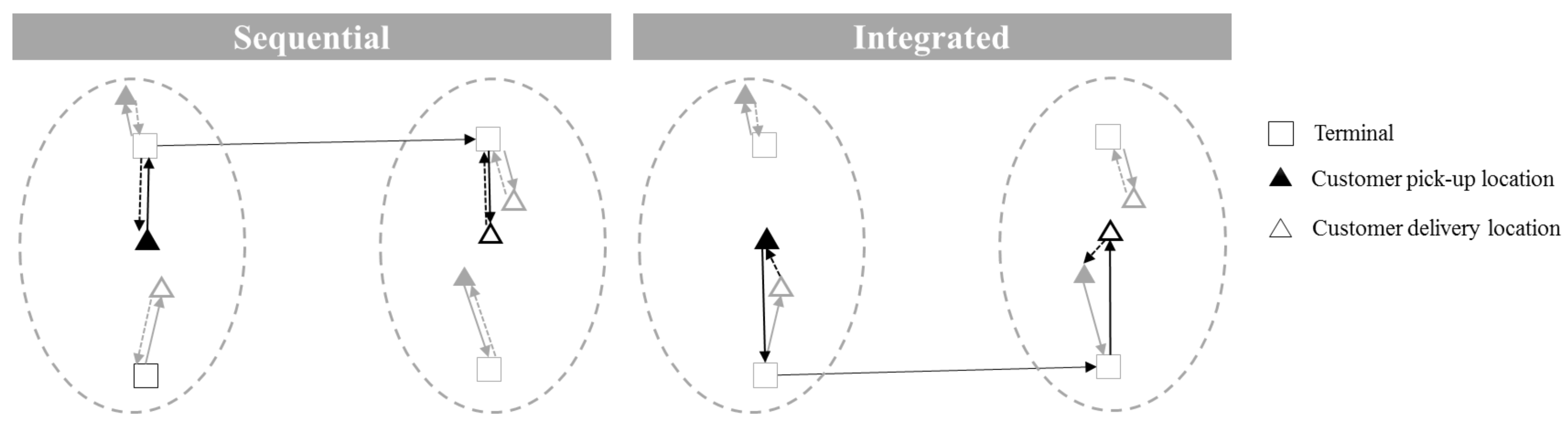
3.1. The Sequential Approach
3.1.1. The Intermodal Long-Haul Routing Problem
3.1.2. Vehicle Routing Problem in Each Region
- a depot node (), identical to
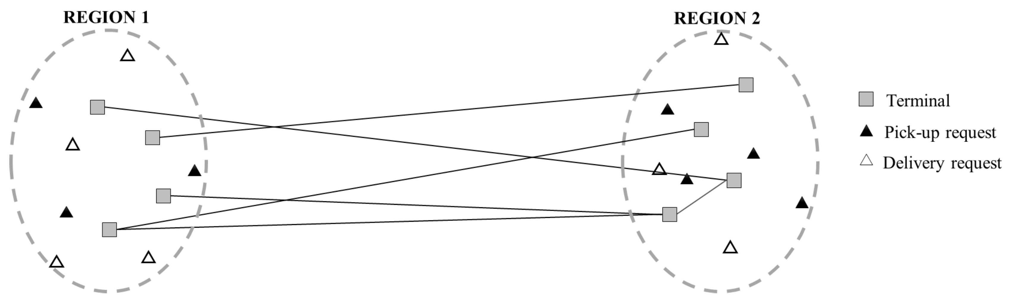
- a pickup task (), which consists of a customer pickup location () and a terminal (), both located in the same service region.
- an delivery task (), which consists of a terminal () and a customer delivery location ().
- a service time , with .
- a cost of visiting a node , with .
- a node type , related to the request dimensions. If the node is a pickup task (, and consequently ), , while if it is a delivery task (, and consequently ).
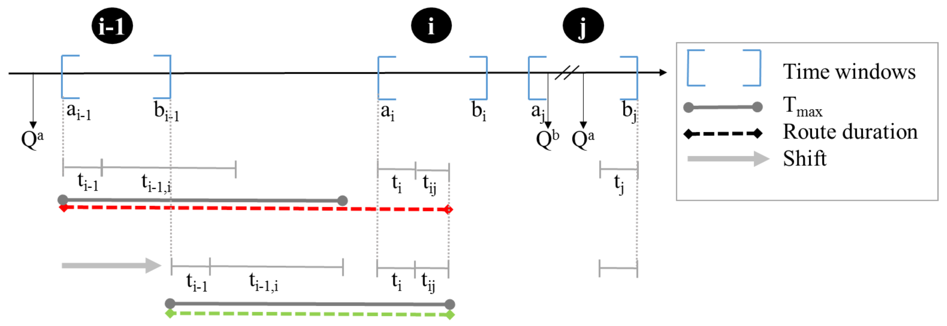
- a time window within which service at node i should start. For pickup tasks (): , . For delivery tasks (): , .
- a rail service , related to node i.
3.2. The Integrated Intermodal Container Routing Problem
4. Large Neighbourhood Search Heuristic Solution Method
4.1. General Structure of the LNS
| Algorithm 1 LNS Heuristic Structure for intermodal routing. |
|
4.2. Integrated Operators
4.3. Preliminary Checks for Inserting a Node
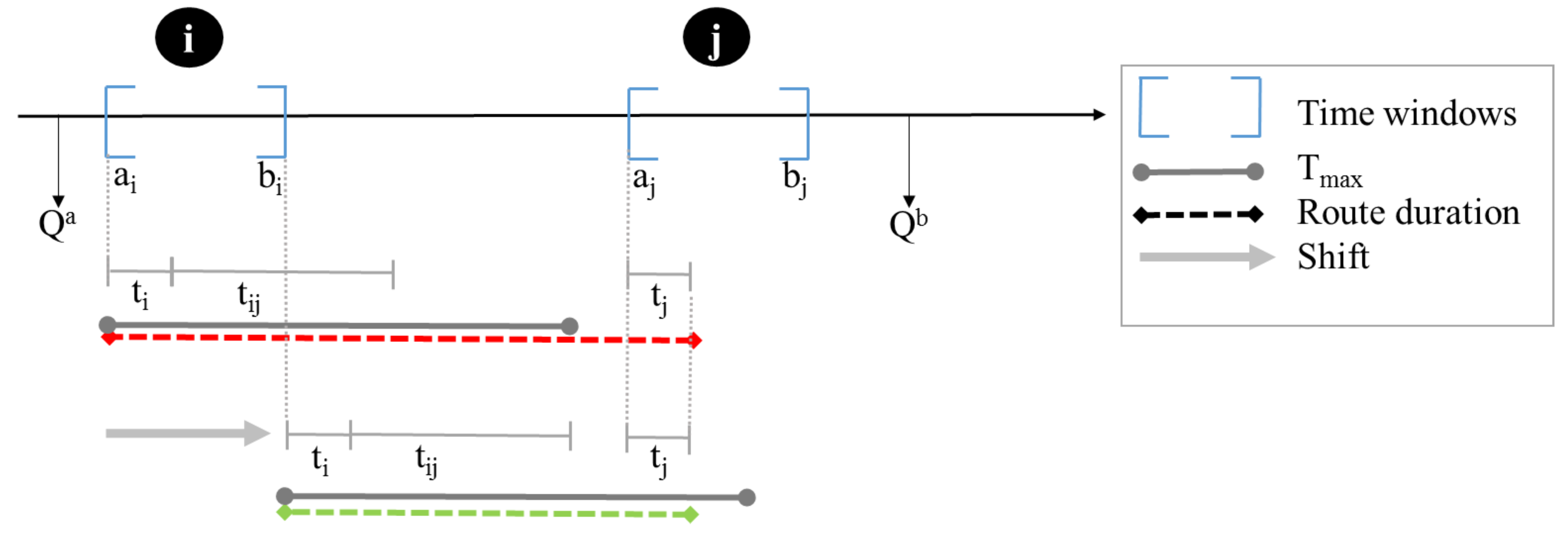
4.4. Feasibility of New Routes
5. Comparison of the Sequential and Integrated Approach
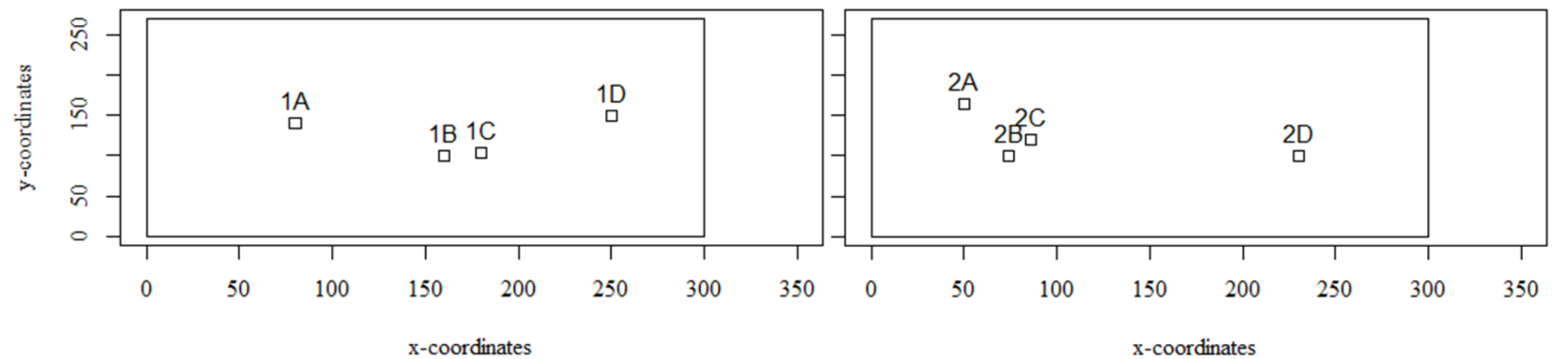
5.1. Generated Instances
5.2. Heuristic Parameters
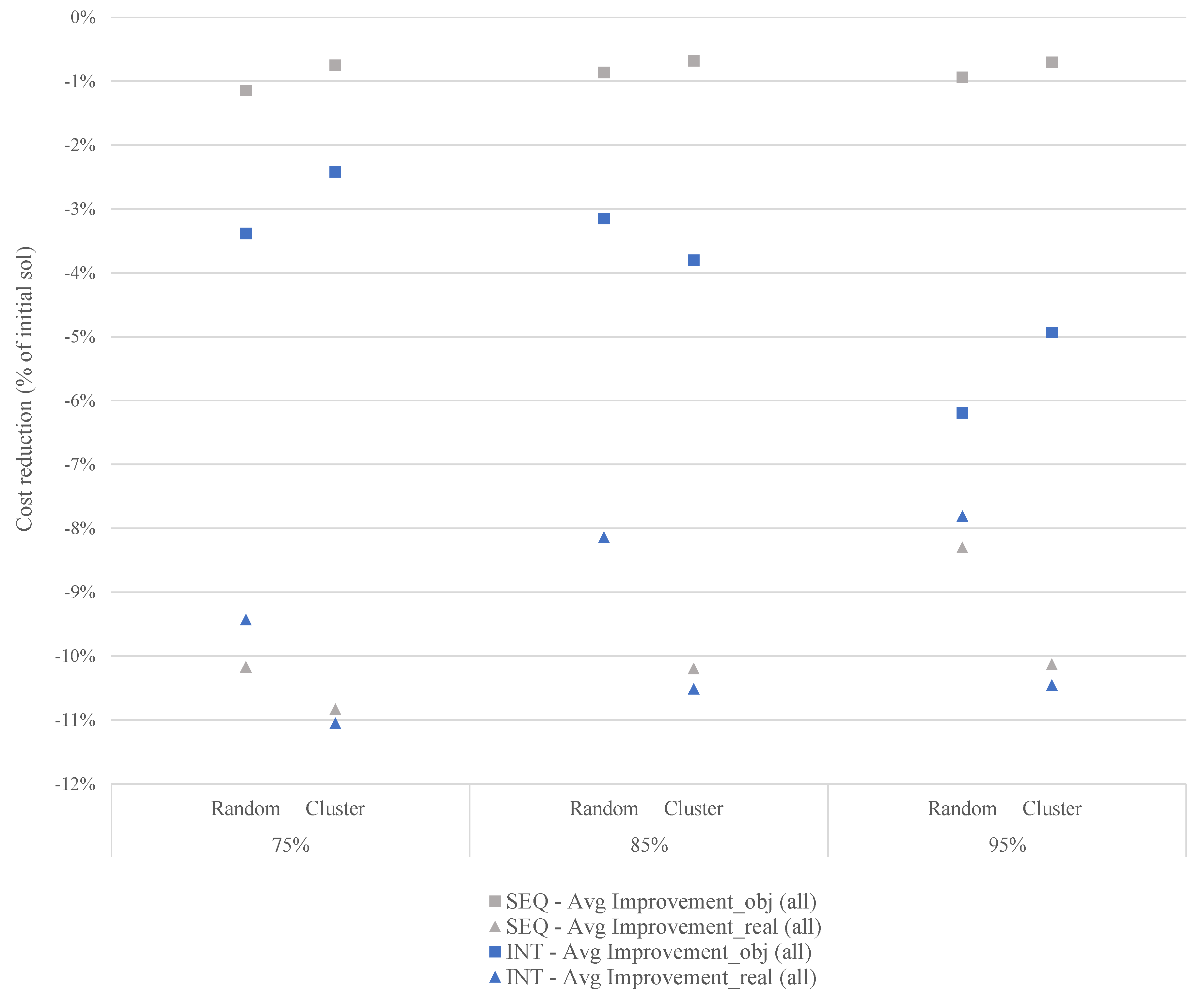
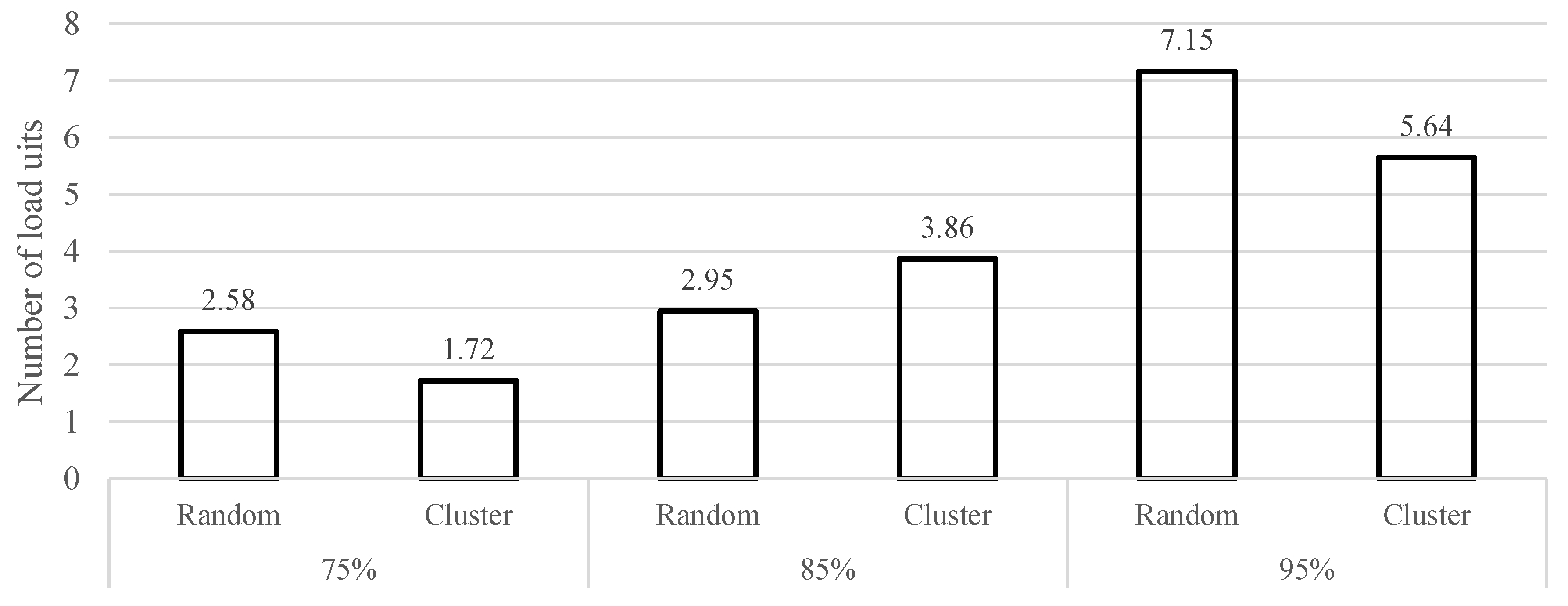
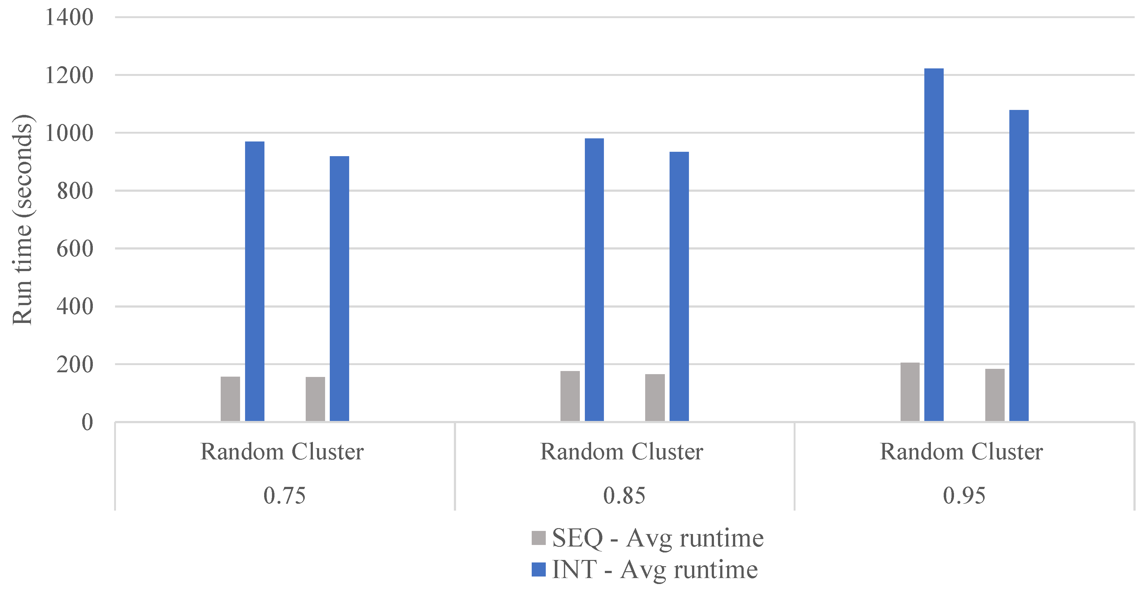
5.3. Experimental Results
6. Case Study: Tactical Service Network Design Decisions
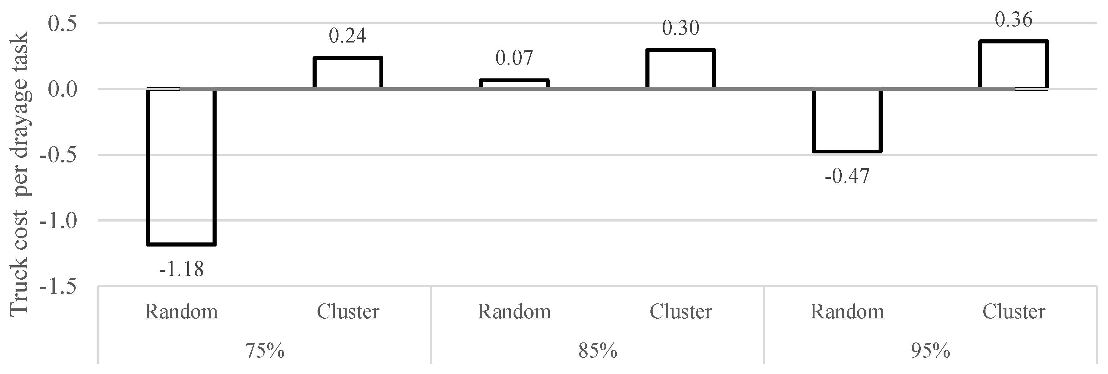
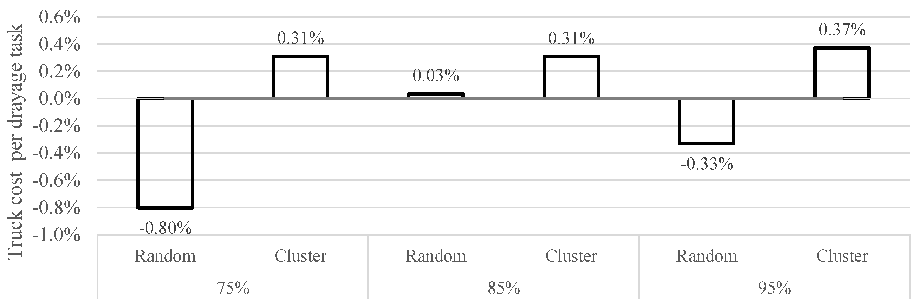
6.1. The Impact of Changes in the Service Network: Removing Long-Haul Services with Small Capacity
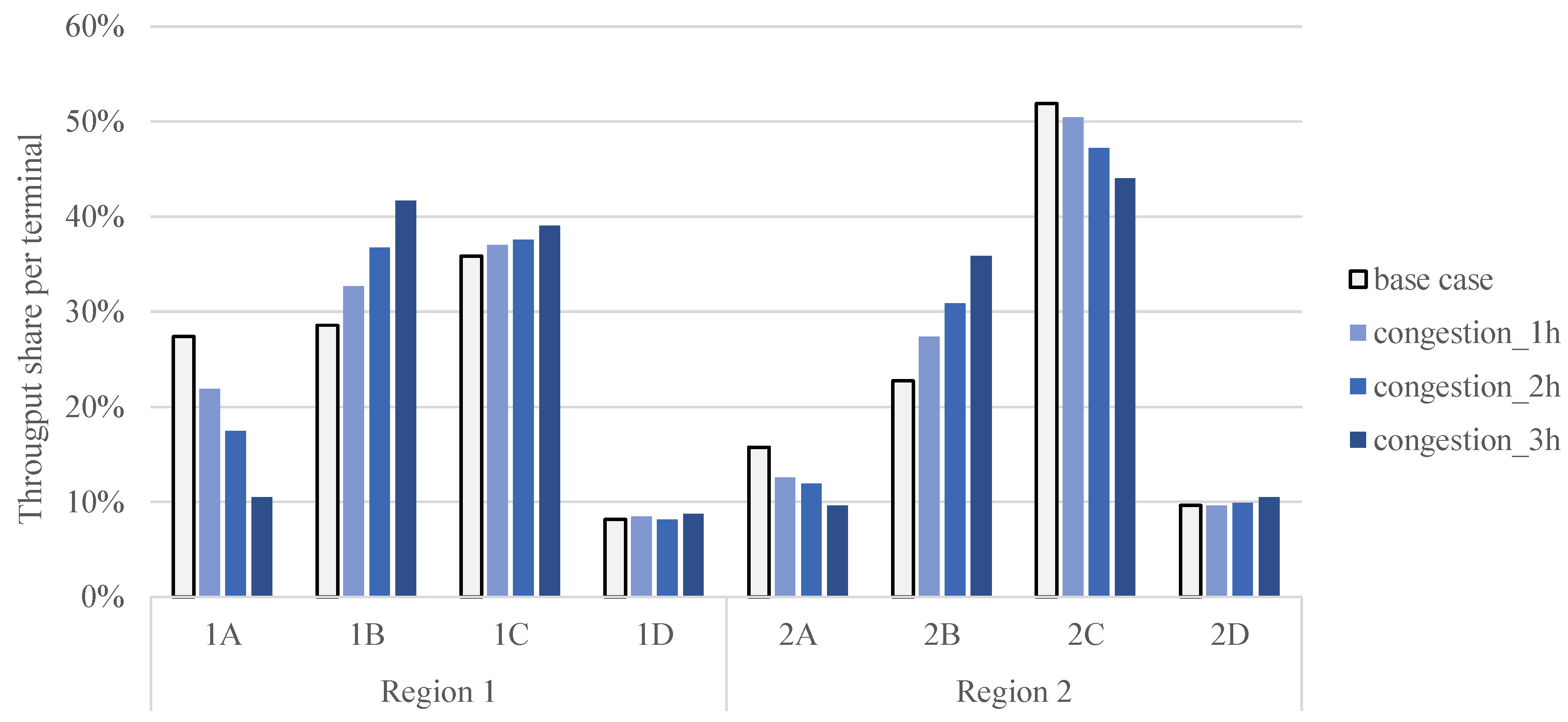
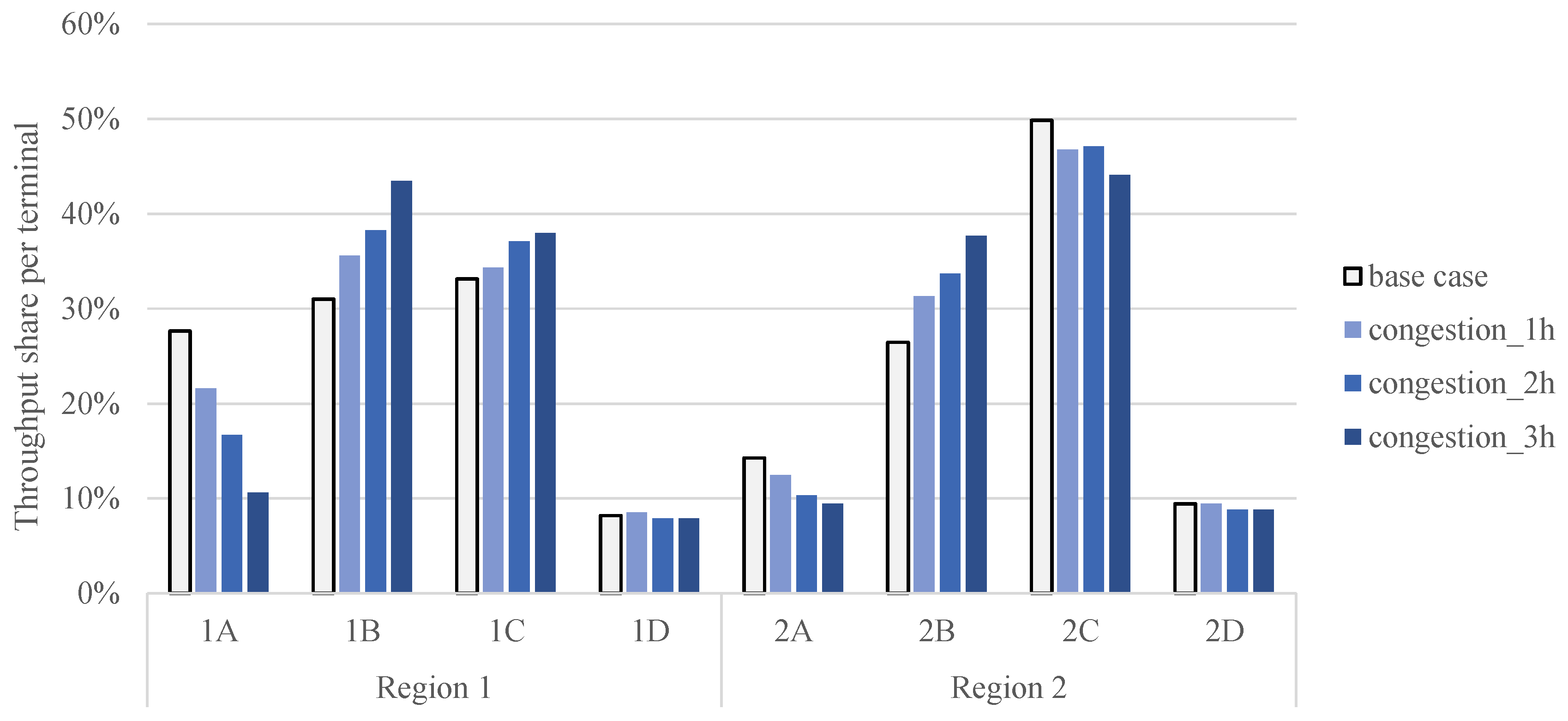
6.2. The Impact of Congestion around Terminals
6.3. Managerial Insights
7. Discussion and Conclusions
Author Contributions
Funding
Acknowledgments
Conflicts of Interest
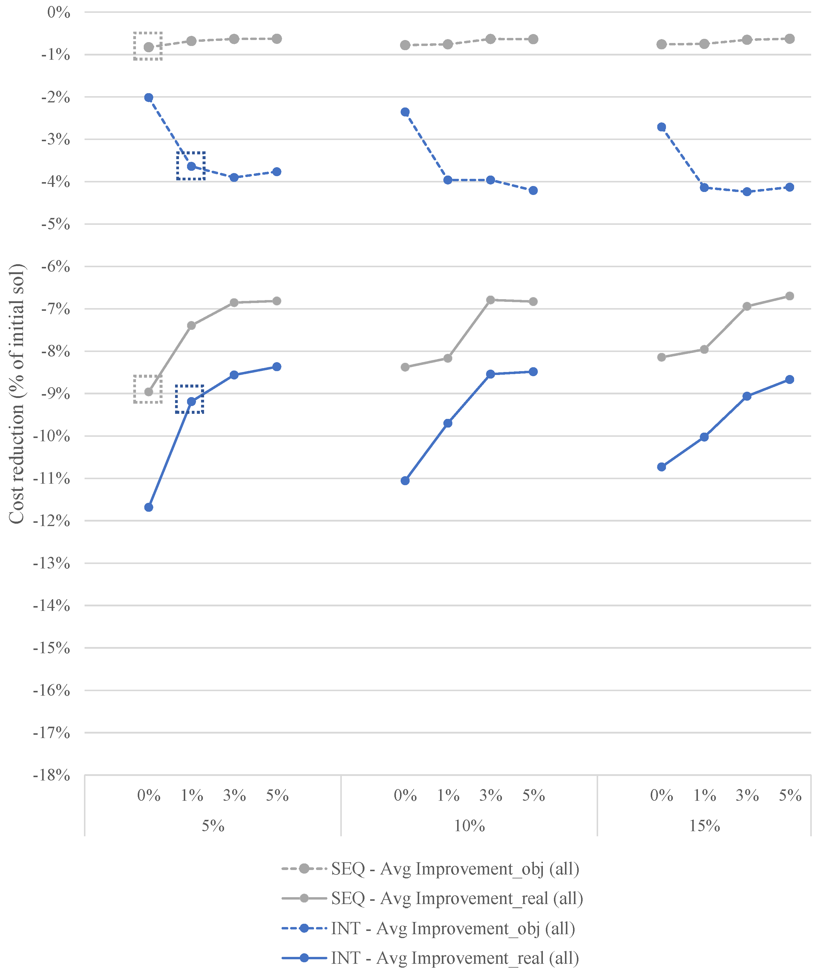
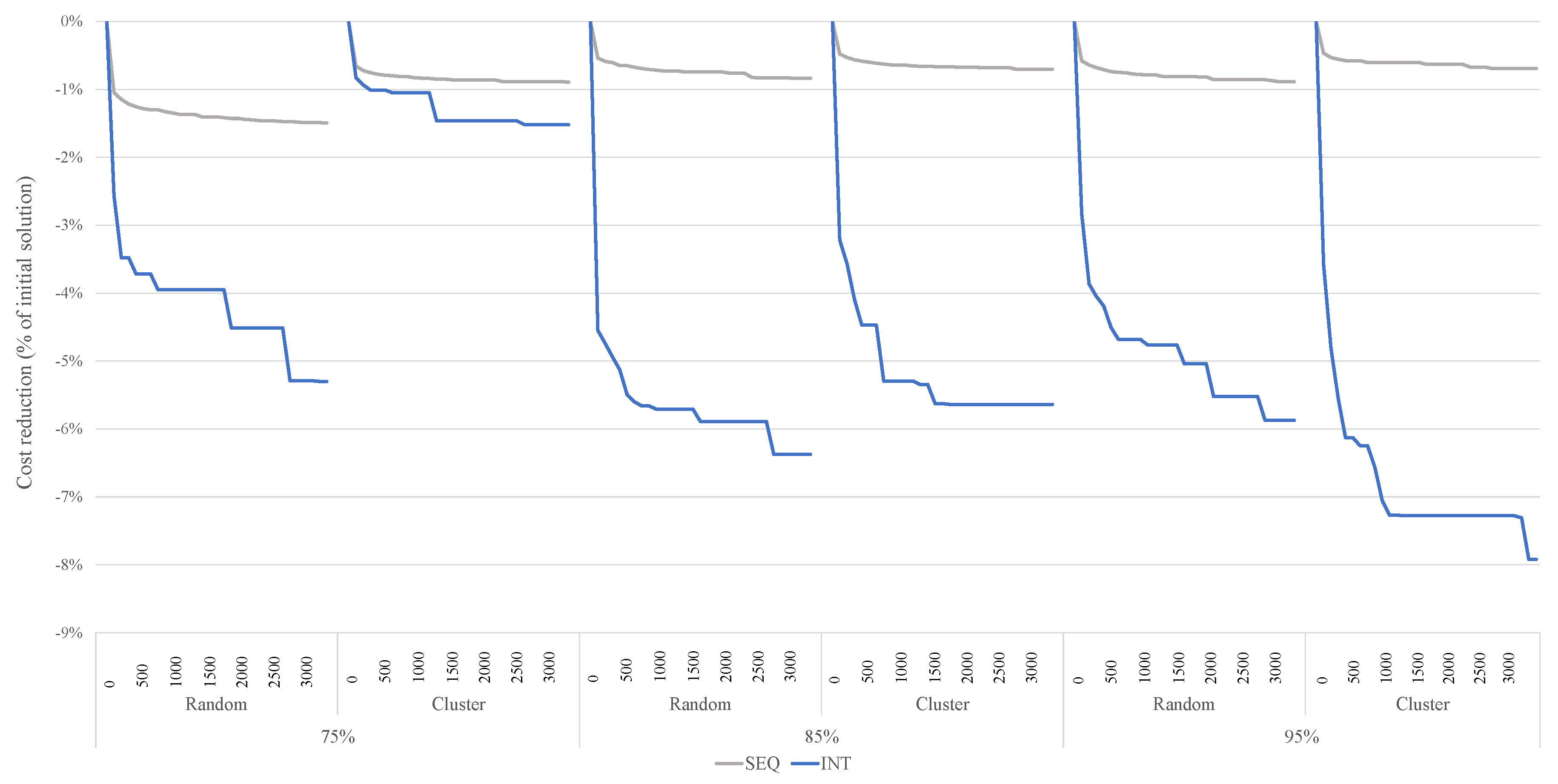
Appendix A. Parameter Tuning
Appendix A.1. Tuning the Parameter Values

| Input Parameter | Tested Values |
|---|---|
| Number of iterations | [0;3000] |
| Removal of requests | 5%; 10%; 15% |
| Acceptance threshold of new solutions | 0%; 1%; 3%; 5% |

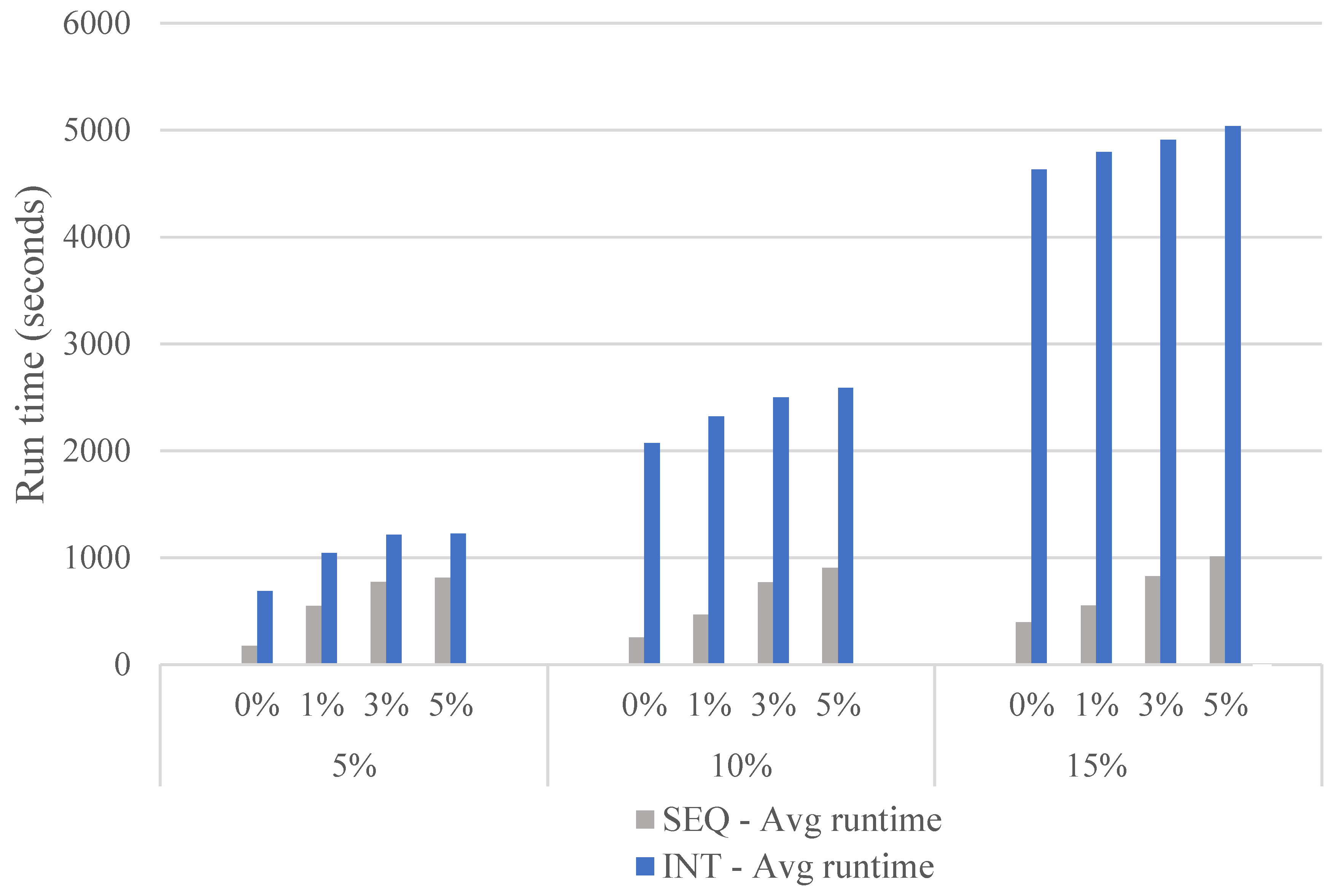
Appendix A.2. The Stopping Criterion

Appendix B. Results for the Congestion Scenario with Clustered Customer Locations

References
- Eurostat. Modal Split of Freight Transport, 2016. Available online: https://ec.europa.eu/eurostat/web/products-datasets/product?code=t2020_rk320 (accessed on 14 March 2019).
- European Commission. MEMO/11/197: Transport 2050: The Major Challenges, the Key Measures, 2011. Available online: http://europa.eu/rapid/press-releaseMEMO-11-197en.htm (accessed on 14 March 2019).
- ITF. ITF Transport Outlook 2015; ITF Transport Outlook; OECD Publishing: Paris, France, 2015. [Google Scholar]
- European Commission. White Paper: A Sustainable Future for Transport—Towards an Integrated, Technology-Led and User Friendly System, 2009. Available online: https://ec.europa.eu/transport/themes/strategies/consultations/2009_09_30_future_of_transport_en (accessed on 14 March 2019).
- Alliance for Logistics Innovation through Collaboration in Europe. Corridors, Hubs and Synchromodality Research and Innovation Roadmap, 2014. Available online: https://www.etp-logistics.eu/wp-content/uploads/2015/08/W26mayo-kopie.pdf (accessed on 14 March 2019).
- Montreuil, B. Toward a Physical Internet: Meeting the global logistics sustainability grand challenge. Logist. Res. 2011, 3, 71–87. [Google Scholar] [CrossRef]
- Ambra, T.; Caris, A.; Macharis, C. Towards freight transport system unification: Reviewing and combining the advancements in the physical internet and synchromodal transport research. Int. J. Prod. Res. 2018, 1–18. [Google Scholar] [CrossRef]
- Caris, A.; Macharis, C.; Janssens, G.K. Planning Problems in Intermodal Freight Transport: Accomplishments and Prospects. Transp. Plan. Technol. 2008, 31, 277–302. [Google Scholar] [CrossRef]
- Caris, A.; Macharis, C.; Janssens, G.K. Decision support in intermodal transport: A new research agenda. Comput. Ind. 2013, 64, 105–112. [Google Scholar] [CrossRef]
- Crainic, T.G.; Kim, K.H. Chapter 8 Intermodal Transportation. In Handbooks in Operations Research and Management Science; Elsevier: Amsterdam, The Netherlands, 2007; Volume 14, pp. 467–537. [Google Scholar]
- Li, L.; Negenborn, R.R.; De Schutter, B. Intermodal freight transport planning—A receding horizon control approach. Transp. Res. Part C Emerg. Technol. 2015, 60, 77–95. [Google Scholar] [CrossRef]
- SteadieSeifi, M.; Dellaert, N.; Nuijten, W.; Van Woensel, T.; Raoufi, R. Multimodal freight transportation planning: A literature review. Eur. J. Oper. Res. 2014, 233, 1–15. [Google Scholar] [CrossRef]
- Heggen, H.; Braekers, K.; Caris, A. A multi-objective approach for intermodal train load planning. OR Spectr. 2018, 40, 341–366. [Google Scholar] [CrossRef]
- van Riessen, B.; Negenborn, R.R.; Dekker, R. Real-time container transport planning with decision trees based on offline obtained optimal solutions. Decis. Support Syst. 2016, 89, 1–16. [Google Scholar] [CrossRef]
- Zhang, M.; Pel, A. Synchromodal hinterland freight transport: Model study for the port of Rotterdam. J. Transp. Geogr. 2016, 52, 1–10. [Google Scholar] [CrossRef]
- Grasman, S.E. Dynamic approach to strategic and operational multimodal routing decisions. Int. J. Logist. Syst. Manag. 2006, 2, 96–106. [Google Scholar] [CrossRef]
- Bock, S. Real-time control of freight forwarder transportation networks by integrating multimodal transport chains. Eur. J. Oper. Res. 2010, 200, 733–746. [Google Scholar] [CrossRef]
- Di Febbraro, A.; Sacco, N.; Saeednia, M. An agent-based framework for cooperative planning of intermodal freight transport chains. Transp. Res. Part C Emerg. Technol. 2016, 64, 72–85. [Google Scholar] [CrossRef]
- Erera, A.L.; Morales, J.C.; Savelsbergh, M. Global intermodal tank container management for the chemical industry. Transp. Res. Part E Logist. Transp. Rev. 2005, 41, 551–566. [Google Scholar] [CrossRef]
- Assadipour, G.; Ke, G.Y.; Verma, M. Planning and managing intermodal transportation of hazardous materials with capacity selection and congestion. Transp. Res. Part E Logist. Transp. Rev. 2015, 76, 45–57. [Google Scholar] [CrossRef]
- Jiang, X.; Bai, R.; Atkin, J.; Kendall, G. A scheme for determining vehicle routes based on Arc-based service network design. INFOR Inf. Syst. Oper. Res. 2017, 55, 16–37. [Google Scholar] [CrossRef]
- Verma, M.; Verter, V.; Zufferey, N. A bi-objective model for planning and managing rail-truck intermodal transportation of hazardous materials. Transp. Res. Part E Logist. Transp. Rev. 2012, 48, 132–149. [Google Scholar] [CrossRef]
- Moccia, L.; Cordeau, J.F.; Laporte, G.; Ropke, S.; Valentini, M.P. Modeling and solving a multimodal transportation problem with flexible-time and scheduled services. Networks 2011, 57, 53–68. [Google Scholar] [CrossRef]
- Chang, T.S. Best routes selection in international intermodal networks. Comput. Oper. Res. 2008, 35, 2877–2891. [Google Scholar] [CrossRef]
- Caramia, M.; Guerriero, F. A heuristic approach to long-haul freight transportation with multiple objective functions. Omega 2009, 37, 600–614. [Google Scholar] [CrossRef]
- van Riessen, B.; Negenborn, R.R.; Dekker, R.; Lodewijks, G. Service network design for an intermodal container network with flexible transit times and the possibility of using subcontracted transport. Int. J. Shipp. Transp. Logist. 2015, 7, 457–477. [Google Scholar] [CrossRef]
- Rudi, A.; Fröhling, M.; Zimmer, K.; Schultmann, F. Freight transportation planning considering carbon emissions and in-transit holding costs: A capacitated multi-commodity network flow model. Euro J. Transp. Logist. 2016, 5, 123–160. [Google Scholar] [CrossRef]
- Caris, A.; Janssens, G. A local search heuristic for the pre- and end-haulage of intermodal container terminals. Comput. Oper. Res. 2009, 36, 2763–2772. [Google Scholar] [CrossRef]
- Toth, P.; Vigo, D. (Eds.) Vehicle Routing: Problems, Methods, and Applications, 2nd ed.; Number 18 in MOS-SIAM Series on Optimization; SIAM [u.a.]: Philadelphia, PA, USA, 2014. [Google Scholar]
- Braekers, K.; Ramaekers, K.; Van Nieuwenhuyse, I. The vehicle routing problem: State of the art classification and review. Comput. Ind. Eng. 2016, 99, 300–313. [Google Scholar] [CrossRef]
- Dotoli, M.; Epicoco, N. A technique for the optimal management of containers’ drayage at intermodal terminals. In Proceedings of the 2016 IEEE International Conference on Systems, Man, and Cybernetics (SMC), Budapest, Hungary, 9–12 October 2016; pp. 566–571. [Google Scholar]
- Pérez Rivera, A.E.; Mes, M.R.K. Scheduling Drayage Operations in Synchromodal Transport. In Computational Logistics; Bektaş, T., Coniglio, S., Martinez-Sykora, A., Voß, S., Eds.; Springer International Publishing: Cham, Switzerland, 2017; Volume 10572, pp. 404–419. [Google Scholar]
- Zhang, R.; Yun, W.Y.; Moon, I. A reactive tabu search algorithm for the multi-depot container truck transportation problem. Transp. Res. Part E Logist. Transp. Rev. 2009, 45, 904–914. [Google Scholar] [CrossRef]
- Zhang, R.; Yun, W.Y.; Kopfer, H. Heuristic-based truck scheduling for inland container transportation. OR Spectr. 2010, 32, 787–808. [Google Scholar] [CrossRef]
- Nossack, J.; Pesch, E. A truck scheduling problem arising in intermodal container transportation. Eur. J. Oper. Res. 2013, 230, 666–680. [Google Scholar] [CrossRef]
- Sterzik, S.; Kopfer, H. A Tabu Search Heuristic for the Inland Container Transportation Problem. Comput. Oper. Res. 2013, 40, 953–962. [Google Scholar] [CrossRef]
- Reinhardt, L.B.; Pisinger, D.; Spoorendonk, S.; Sigurd, M.M. Optimization of the drayage problem using exact methods. INFOR Inf. Syst. Oper. Res. 2016, 54, 33–51. [Google Scholar] [CrossRef]
- Shiri, S.; Huynh, N. Optimization of drayage operations with time-window constraints. Int. J. Prod. Econ. 2016, 176, 7–20. [Google Scholar] [CrossRef]
- Francis, P.; Zhang, G.; Smilowitz, K. Improved modeling and solution methods for the multi-resource routing problem. Eur. J. Oper. Res. 2007, 180, 1045–1059. [Google Scholar] [CrossRef]
- Braekers, K.; Caris, A.; Janssens, G.K. Integrated planning of loaded and empty container movements. OR Spectr. 2013, 35, 457–478. [Google Scholar] [CrossRef]
- Posada, M.; Andersson, H.; Häll, C.H. The integrated dial-a-ride problem with timetabled fixed route service. Public Transp. 2017, 9, 217–241. [Google Scholar] [CrossRef]
- Medina, J.; Hewitt, M.; Lehuédé, F.; Péton, O. Integrating long-haul and local transportation planning: The Service Network Design and Routing Problem. EURO J. Transp. Logist. 2018. [Google Scholar] [CrossRef]
- Dragomir, A.G.; Nicola, D.; Soriano, A.; Gansterer, M. Multidepot pickup and delivery problems in multiple regions: A typology and integrated model. Int. Trans. Oper. Res. 2018, 25, 569–597. [Google Scholar] [CrossRef]
- Soriano, A.; Gansterer, M.; Hartl, R.F. The two-region multi-depot pickup and delivery problem. OR Spectr. 2018. [Google Scholar] [CrossRef]
- Wolfinger, D.; Tricoire, F.; Doerner, K.F. A matheuristic for a multimodal long haul routing problem. EURO J. Transp. Logist. 2018. [Google Scholar] [CrossRef]
- Shaw, P. Using Constraint Programming and Local Search Methods to Solve Vehicle Routing Problems. In Principles and Practice of Constraint Programming—CP98; Goos, G., Hartmanis, J., van Leeuwen, J., Maher, M., Puget, J.F., Eds.; Springer: Berlin/Heidelberg, Germany, 1998; Volume 1520, pp. 417–431. [Google Scholar]
- Ropke, S.; Pisinger, D. An Adaptive Large Neighborhood Search Heuristic for the Pickup and Delivery Problem with Time Windows. Transp. Sci. 2006, 40, 455–472. [Google Scholar] [CrossRef]
- Savelsbergh, M.W.P. The Vehicle Routing Problem with Time Windows: Minimizing Route Duration. ORSA J. Comput. 1992, 4, 146–154. [Google Scholar] [CrossRef]
- Vidal, T.; Crainic, T.G.; Gendreau, M.; Prins, C. Timing problems and algorithms: Time decisions for sequences of activities. Networks 2015, 65, 102–128. [Google Scholar] [CrossRef]
- Cordeau, J.F.; Gendreau, M.; Laporte, G. A tabu search heuristic for periodic and multi-depot vehicle routing problems. Networks 1997, 30, 105–119. [Google Scholar] [CrossRef]


| Class | Locations | Demand Level |
|---|---|---|
| 1 | random | 75% |
| 2 | cluster | 75% |
| 3 | random | 85% |
| 4 | cluster | 85% |
| 5 | random | 95% |
| 6 | cluster | 95% |
| Input Parameter | Value |
|---|---|
| [0;6*24] h | |
| 2 h | |
| 1 h | |
| 0 h | |
| 15 h | |
| 6 h | |
| 1 euro per km |
| Input Parameter | Sequential | Integrated |
|---|---|---|
| Number of iterations | 3000 | 3000 |
| Acceptance threshold of new solutions | 0% | 1% |
| Removal of requests | 5% | 5% |
| Base | a | b | ||
|---|---|---|---|---|
| Random | TC_obj | 1,315,115.29 | 1,316,977.03 | 1,330,566.26 |
| TC_real | 144,115.29 | 144,921.47 | 148,366.26 | |
| vrpCost | 108,755.37 | 109,088.22 | 111,905.62 | |
| directTruckCost | 21,381.42 | 21,959.91 | 22,486.64 | |
| Nbr requests (this week) | 257.10 | 253.57 | 255.78 | |
| Cluster | TC_obj | 1,304,305.69 | 1,314,235.72 | 1,328,823.97 |
| TC_real | 137,305.69 | 144,423.22 | 147,712.86 | |
| vrpCost | 103,223.35 | 108,734.29 | 111,374.22 | |
| directTruckCost | 20,145.84 | 21,832.68 | 22,380.31 | |
| Nbr requests (this week) | 256.30 | 253.52 | 255.67 |
© 2019 by the authors. Licensee MDPI, Basel, Switzerland. This article is an open access article distributed under the terms and conditions of the Creative Commons Attribution (CC BY) license (http://creativecommons.org/licenses/by/4.0/).
Share and Cite
Heggen, H.; Molenbruch, Y.; Caris, A.; Braekers, K. Intermodal Container Routing: Integrating Long-Haul Routing and Local Drayage Decisions. Sustainability 2019, 11, 1634. https://doi.org/10.3390/su11061634
Heggen H, Molenbruch Y, Caris A, Braekers K. Intermodal Container Routing: Integrating Long-Haul Routing and Local Drayage Decisions. Sustainability. 2019; 11(6):1634. https://doi.org/10.3390/su11061634
Chicago/Turabian StyleHeggen, Hilde, Yves Molenbruch, An Caris, and Kris Braekers. 2019. "Intermodal Container Routing: Integrating Long-Haul Routing and Local Drayage Decisions" Sustainability 11, no. 6: 1634. https://doi.org/10.3390/su11061634
APA StyleHeggen, H., Molenbruch, Y., Caris, A., & Braekers, K. (2019). Intermodal Container Routing: Integrating Long-Haul Routing and Local Drayage Decisions. Sustainability, 11(6), 1634. https://doi.org/10.3390/su11061634