Distribution-Free Stochastic Closed-Loop Supply Chain Design Problem with Financial Management

Abstract

Financial flow is an important part of supply chain management (SCM) and increasingly playing a crucial role as the amount of global trade increases. Reasonable and scientific financial operation is necessary in closed-loop supply chain management, especially when customer demand is uncertain. However, financial flow, which may lead to an increase in effectiveness, has rarely been considered in the literature. In this paper, we present a closed-loop supply chain design with financial management problem, which is tackled as a stochastic programming model with ambiguity demand set. The main contributions of this work include: (i) A joint chance constrained programming model is proposed to maximize the total profit, and (ii) financial flow and uncertain demand are both taken into consideration. According to the characteristic of the problem, we chose four approaches, namely sample average approximation (SAA), enhanced sample average approximation (ESAA), Markov approximation (MA), and mixed integer second-order conic program (MI-SOCP). Computational experiments were conducted to compare the adopted methods, and 10,000 scenarios were generated to examine the reliability of the methods. Numerical results revealed that the Markov approximation approach can achieve more reliable solutions.

1. Introduction

With the development of the global economy, market competition is becoming fiercer and fiercer. In order to maximize the profit of the enterprise, firms’ decision makers have to deal with the following tasks: Where to locate the facility (i.e., warehouse, distribution center location), how to cut costs, and how to improve customer service. In this situation, a lot of literature related with the topic of supply chain management has to be closely watched by academics and industry researchers.

In general, the supply chain management (SCM) problem just only concerned with the quantities of procurement, production, inventory, and transportation among the different sections. However, along with the constant consumption of resources, the problem of pollution control, waste recycling, and social responsibility becomes extremely important. Therefore, the closed-loop supply chain (CLSC) plays an increasingly crucial role in real life. It can guarantee the least waste of materials through following the conservation laws during the life of the materials.

In face, material flow, information flow, and financial flow are the three major parts of the supply chain problem. While material and information movements have a series of research in the context of CLSC, financial movement has rarely appeared in relevant literature. Finance management is an important factor in improving the efficiency of supply chain networks. According to the World Bank report, supply chain finance can improve trading opportunities for companies [1].

Many well-known companies have integrated financial management into their supply chain system, such as Intel, GE, and Deutz. For example, Intel asserted integration of material and finical flows into an information system, and GE improvee its account payable by 12% though an electronic invoice system, which help them to predict the cash liquidity required. In addition, Deutz combined the financial flow with their inventory levels [2].

Reasonable and scientific financial operations are necessary in closed-loop supply chain management, especially when the customer demand is uncertain. Traditionally, it is assumed that the demand is deterministic in supply chain finance problems. In reality, however, demand is usually uncertain due to complex market environments. Additionally, as the historical data may be inadequate or may not be fully accessed, we cannot accurately estimate the distribution of demand. Based on the above discussions, this paper considers uncertain customer demand without distribution. We portray the uncertain demand via a wildly used ambiguity set, which only uses the empirical mean and variance information.

To the best of our knowledge, we are the first to consider finance in a closed-loop supply chain and ambiguous customers simultaneously. The contributions of this paper are four aspects as follows:

(1)

The closed-loop supply chain problem with a financial aspect is proposed and studied. The customer demand is uncertain, only knowing the mean and covariance of the demand. A joint chance-constrained model is proposed.

(2)

For the problem, we adopted four approaches to handle the chance constraints. The four methods were: Sample average approximation (SAA), enhanced sample average approximation (ESAA), Markov approximation (MA), and mixed integer second-order conic program (MI-SOCP).

(3)

Numerical experiments on randomly generated instances were conducted to examine the reliability of the proposed methods. Computational results showed the efficiency of the four adopted solution approaches.

(4)

Sensitivity analysis was conducted on the impact of CLSC with the variation rate of recycling and producing.

The remainder of this paper is arranged as follows. Section 2 reviews the existing financial literature in SCM, and then addresses the studies of the CLSC problem. Closed-loop supply chain with a financial management problem and model is formally described in Section 3. We introduce the four approximation methods in the Section 4. Section 5 illustrates the performance of the four methods and makes a sensitivity analysis, as well. Finally, we report the conclusions of this work and indicate some future research directions in Section 6.

2. Literature Review

In this section, we categorize the literature into three aspects. The first category addresses the studies considering financial issues in supply chain; the second is relevant to closed-loop supply chain design; the final section is related to the approach of solving the distribution-free model.

2.1. Working Capital Management in Supply Chain

Working capital management (WCM) is important for enterprises when they face financical difficulties, especially with increased economic uncertainty. Botoc and Anton (2017) [3] examined the relationship between working capital management and firm profitability. They used a panel data set on high-growth firms(HGFs) from Central, Eastern, and South-Eastern Europe during the time span 2006–2015 and found an inverted U-shape relationship between working capital level and firm profitability. Their findings indicated that HGFs should find and maintain the optimal working capital level that maximizes their profitability. Aktas et al. (2015) [4] examined the value effect of working capital management for a large sample of US firms between 1982–2011, and their results indicated (i) the existence of an optimal level of working capital policy, and that (ii) firms that converge to that optimal level improve their stock and operating performance. Lind et al. (2012) [5] examined working capital management using financial value chain analysis by cycle times in the value chain of the automotive industry during 2006–2008. According to their study, the change of cycle times of working capital followed mainly the change of cycle time of inventories. Julius et al. (2014) [6] examined the role of business cycles on the working capital–profitability relationship using a sample of Finnish listed companies over an 18-year period, and they found the impact of business cycle on the working capital–profitability relationship is more pronounced in economic downturns relative to economic boom. Further, they showed that the significance of efficient inventory management and accounts receivables conversion periods increases during periods of economic downturns. Ding et al. (2013) [7] used a panel of over 116,000 Chinese firms of different ownership types over the period 2000–2007 to analyze the linkages between investment in fixed and working capital and financing constraints, and they found that those firms characterized by high working capital display high sensitivities of investment in working capital to cash flow and low sensitivities of investment in fixed capital to cash flow.

2.2. Closed-Loop Supply Chain

In recent years, commercial competition is increasingly fierce. A solution that improves the supply chain value is important. In the following, we address the literature associated with closed-loop supply chain design.

Hasanov et al. (2019) [8] addressed the coordination of order quantities in a four-level closed-loop supply chain (CLSC) with remanufacturing. The levels were multiple buyers and tier-1 and tier-2 suppliers, and a manufacturer. The reverse channel consisted of an inspection and disassembly center and a remanufacturing center. Customer demand was met from either newly manufactured items, remanufacturing used items collected from customers for recovery, or from both. The results showed that higher collection rates of used items reduced the supply chain costs and improved its environmental performance.

Modak et al. (2019) [9] took a practical step in the implementation of a corporate social responsibility (CSR) activity. They developed a socially responsible closed-loop supply chain (CLSC) model that takes into account donation, as a CSR activity, and recycling of the used products for environmental sustainability.

Gaur and Mani (2018) [10] proposed a conceptual framework, discussing the major threats and opportunities for business firms engaged in a CLSC operation, and their results suggested that there are seven driving forces for a closed-loop supply chain. The proposed conceptual framework serves as a decision making tool and intends to help both academicians and practitioners, as it highlights major research issues in this field. Finally, managerial implications and future research directions were outlined.

Liu et al. (2018) [11] devised a green closed-loop supply chain (GCLSC) with uncertain demand considering environmental problems. In their problem, two conflict objectives and recycling used products were considered. To solve this problem, they developed three algorithms: The e-constraint method, the nondominated sorting genetic algorithm (NSGA-II), and the multiobjective simulated annealing method (MOSA).

Bottani and Casella (2018) [12] investigated the issue of minimizing the environmental burden of a real closed-loop supply chain (CLSC), consisting of a pallet provider, a manufacturer, and several retailers. A simulation model was developed under Microsoft Excel (TM) to reproduce the flow of returnable transport items (RTIs) in the CLSC and to compute the corresponding environmental impact.

2.3. Distribution-Free Approach

Due to the fact that the probability distribution of demand may not be accurately estimated, some researchers proposed a distribution roubust approach with partial information of stochastic parameters.

Wagner (2008) [13] proposed an approximation method to the chance constraint under unknown distribution with only limited distributional information, i.e., the mean and covariance matrix. Delage and Ye (2010) [14] first introduced a moment-based ambiguity set to describe the uncertainty, in which the first- and the second-order moments correspond to the mean vector and covariance matrix. Ng (2015) [15] approximated the chance constraint such that the mean and the standard deviation of shipping demand were provided. Zheng et al. (2016) [16] used multiple scenarios to approximate the uncertainty, i.e., adopting the sample average approximation method. Zhang et al. (2018) [17] applied a 0–1 SOCP approximation method to solve the appointment scheduling under stochastic service duration with unknown distributions to minimize the expected total waiting time.

Most of the literature about the relationship between working capital management and firm performance is empirical research. Different from the literature mentioned above, in this work, we proposed a novel mathematical programming model considering financial management. Moreover, we considered the uncertainty in customer demand which can depict the real business environment in real life. To the best of our knowledge, there is no result for the distribution-free stochastic closed-loop supply chain design problem with financial management.

3. Problem Definition and Model Formulation

In this section, we first start with defining the problem and follow that with the formulation of a stochastic closed-loop supply chain with finance factors.

3.1. Problem Description

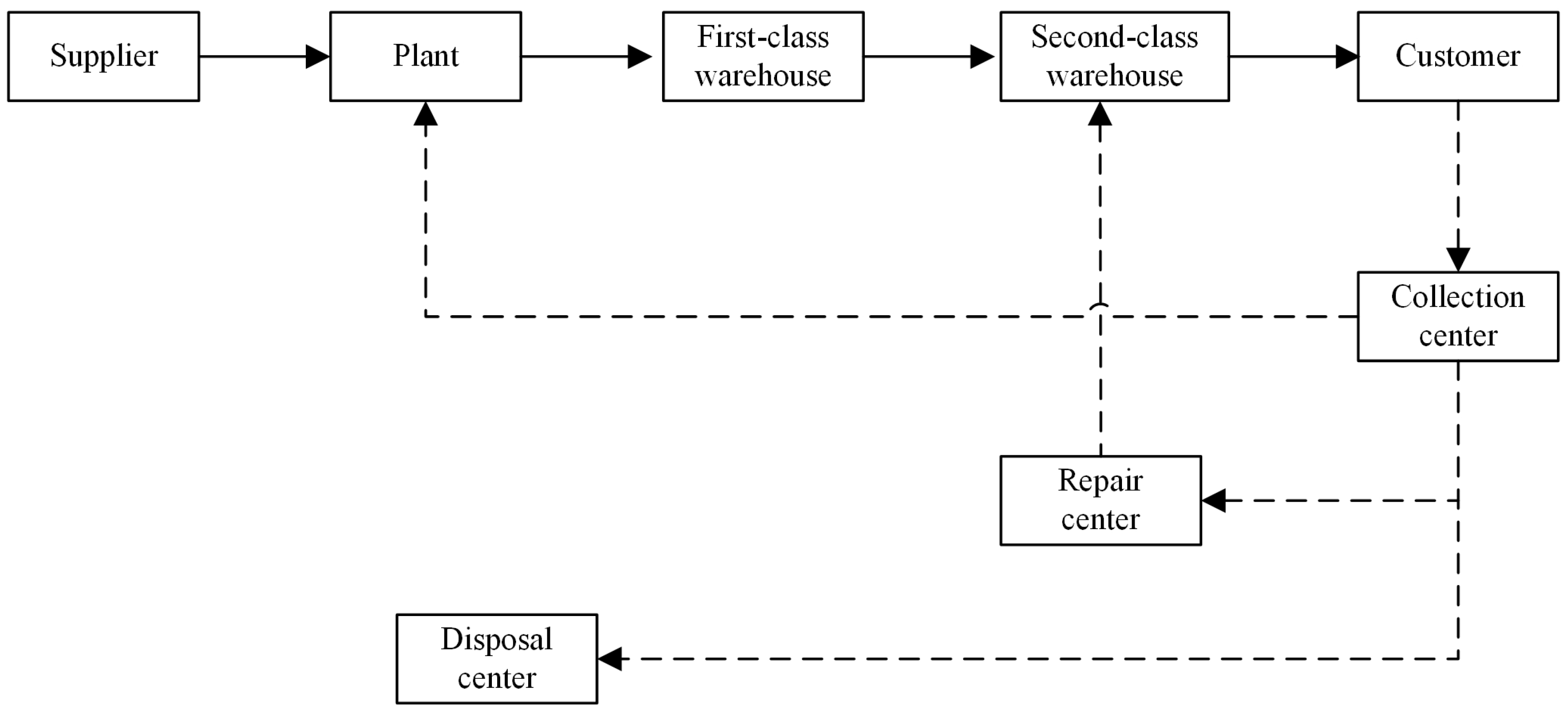
The structure of a closed-loop supply chain network is illustrated in Figure 1. In this holistic closed-loop supply chain finance problem, the decision makers firstly need to decide which suppliers should be selected, and the location of plant, first-warehouse, second-class warehouse, and collection center. Then, the suppliers are responsible for providing raw material to the plant and a conversion rate ${\beta }_1$ is given from raw materials to products. After that, the products are shipped from plant to customer through the first-class warehouse and second-class warehouse. The ratio of ${\beta }_2$ recycled product from customer is transferred to the collection center for classifying and inspecting. After inspecting in the collection center, a percentage of ${\beta }_3$ products are shipped to the plant for remanufacturing, and a proportion of ${\beta }_4$ products are sent to the repair center. After being repaired, they are shipped to the second-class warehouse for sale again. Finally, a percentage of ${\beta }_5$ products are shipped to the disposal center. Using methods like this, the returmed products can be directly delivered to the related centers, which can cut a lot of operational cost for the firm.

Concerning the financial aspect, we concentrate mainly on two levels: fFow-in cash and flow-out cash. In this problem, we assume that flow-in cash includes credit and profit in period t, and accounts receivable in period $t-1$. Similarly, flow-out cash includes interest, repayment of capital, and operation cost.

In order to portray this problem in a way that makes more sense, we considered the customer demand as uncertain, and a time-varying volatility in product price, operation cost, interest, and so on. To show the proposed model with more details, we present the stochastic cloosed-loop supply chain with financial in the following section.

3.2. Mathematical Model

In this section, we first introduce the concept of moment-based ambiguity set and then a new stochastic model is presented.

3.2.1. Moment-Based Ambiguity Set

In a real business situation, the probability distribution of consumer demand may not be accurately estimated, especially with e-commerce. Therefore, we introduced a moment-based ambiguity set to describe the demand uncertainty. Let $\mathsf{\Omega }$ and $\omega$ denote the set of samples and the index of sample, respectively, and $\left|\mathsf{\Omega }\right|$ denote the cardinality of set $\mathsf{\Omega }$. Thus, for customer demand $D_{nt}$, the historical data of demand are assumed ${\left\{{\mathbf{D}}^{\omega }\right\}}_{\omega =1}^{\left|\mathsf{\Omega }\right|}$, ${\mathbf{D}}^{\omega }={\{D_{11}^{\omega },D_{12}^{\omega },\dots ,D_{nt}^{\omega }\}}^T$, where $D_{nt}^{\omega }$ is the demand of customer n with period t in scenario $\omega$. The mean vector $\mu$ and variance vector $\Sigma$ of demand can be estimated as:

$$\mathbf{\mu }=\frac{1}{\left|\mathsf{\Omega }\right|}·\sum _{\omega \in \mathsf{\Omega }}{\mathit{D}}^{\omega },\mathbf{\Sigma }=\frac{1}{\left|\mathsf{\Omega }\right|}·\sum _{\omega \in \mathsf{\Omega }}({\mathit{D}}^{\omega }-\mathbf{\mu }){({\mathit{D}}^{\omega }-\mathbf{\mu })}^T.$$

As the number of samples $\left|\mathsf{\Omega }\right|$ increases, $\mathbf{\mu }$ and $\mathbf{\Sigma }$ converge to the true mean and covariance of demand as $\left|\mathsf{\Omega }\right|\to \infty$. Therefore, the following ambiguity set includes all probability distributions of demand ${\Xi }_{nt}({\mu }_{nt},{\Sigma }_{nt})$ of customer demand $D_{nt}$, which can be described as:

$${\Xi }_{nt}({\mu }_{nt},{\Sigma }_{nt})=\left\{\begin{array}{cc}{\mathbb{P}}_{nt}:& \begin{array}{l}{\mathbb{E}}_{{\mathbb{P}}_{nt}}\left[D_{nt}\right]={\mu }_{nt}\\ {\mathbb{E}}_{{\mathbb{P}}_{nt}}\left[(D_{nt}-{\mu }_{nt}){(D_{nt}-{\mu }_{nt})}^T\right]={\Sigma }_{nt}\end{array}\end{array}\right.,$$

where ${\mathbb{P}}_{nt}$ denotes the set of all possible probability distribution of customer demand $D_{nt}$ satisfying the given conditions, and $\mathbb{E}[·]$, with respect to ${\mathbb{P}}_{nt}$, denotes the expected value of the expression in the brackets.

3.2.2. Programming Formulation

In this part, we firstly define problem parameters and decision variables, and then propose the distribution-free model for the problem.

Problem parameters:

• T: Set of time period.
• I: Set of supplier.
• J: Set of palnt.
• K: Set of first-class warehouse.
• M: Set of second-class warehouse.
• N: Set of customer.
• E: Set of collection center.
• $p_t$: The market price of products, changing with the period t.
• $C{M}_{it}^S$: The cost of material of supplier i in period t.
• $C{P}_{jt}^P$: The production cost of plant j in period t.
• $C{S}_{kt}^{FC}$: The store cost of first-class warehouse k in period t.
• $C{S}_{mt}^{SC}$: The store cost of second-class warehouse m in period t.
• $C{C}_{et}^{CC}$: The cost of collection center e in period t.
• $C{R}_t^{RC}$: The repair cost in period t.
• $C{D}_t^{DC}$: The disposal cost in period t.
• $F{C}_i^S$: The fixed cost of supplier i.
• $F{C}_j^P$: The fixed cost of plant j.
• $F{C}_k^{FC}$: The fixed cost of first-class warehouse k.
• $F{C}_m^{SC}$: The fixed cost of second-class warehouse m.
• $F{C}_e^{CC}$: The fixed cost of collection center e.
• $F{C}^{CU}$: The fixed cost of each customer service center.
• $F{C}^{RC}$: The fixed cost of repair center.
• $F{C}^{DC}$: The fixed cost of disposal center.
• $T{C}_{ijt}^S$: The transportation cost from supplier i to plant j in period t.
• $T{C}_{jkt}^P$: The transportation cost from plant j to first-class warehouse k in period t.
• $T{C}_{kmt}^{FC}$: The transportation cost from first-class warehouse k to second-class warehouse m in period t.
• $T{C}_{mnt}^{SC}$: The transportation cost from second-class warehouse m to customer n in period t.
• $T{C}_{net}^{CU}$: The transportation cost from customer n to collection center e in period t.
• $T{C}_{ejt}^{CP}$: The transportation cost from collection center e to plant j in period t.
• $T{C}_{et}^{CR}$: The transportation cost from collection center e to repair center in period t.
• $T{C}_{mt}^{RSC}$: The transportation cost from repair center to second-class warehouse m in period t.
• $T{C}_{et}^{CD}$: The transportation cost from collection center e to disposal center in period t.
• $\varsigma$: A sufficiently large positive number.
• ${\beta }_1$: The conversion ratio from raw materials to end products.
• ${\beta }_2$: The recycling rate of products from customer to collection center.
• ${\beta }_3$: The transform rate of products from collection center to plant.
• ${\beta }_4$: The transform rate of products from collection center to repair center.
• ${\beta }_5$: The transform rate of products from collection center to disposal.
• ${\gamma }_1$: The payment ratio when products are sold.
• ${\gamma }_2$: The proportion of accounts receivable.
• $C_{nt}$: The unit penalty cost of the superfluous products.

Decision variables:

• $Q_{ijt}^S$: The transportation volume from supplier i to plant j in period t.
• $Q_{jkt}^P$: The transportation volume from plant j to first-class warehouse k in period t.
• $Q_{kmt}^{FC}$: The transportation volume from first-class warehouse k to second-class warehouse m in period t.
• $Q_{mnt}^{SC}$: The transportation volume from second-class warehouse m to customer n in period t.
• $Q_{net}^{CU}$: The transportation volume from customer n to collection center e in period t.
• $Q_{ejt}^{CP}$: The transportation volume from collection center e to plant j in period t.
• $Q_{et}^{CR}$: The transportation volume from collection center e to repair center in period t.
• $Q_{mt}^{RSC}$: The transportation volume from repair center to second-class warehouse m in period t.
• $Q_{et}^{CD}$: The transportation volume from collection center e to diaposal center in period t.
• $S_{kt}^{FC}$: The store volume of first-class warehouse k in period t.
• $S_{mt}^{SC}$: The store volume of second-class warehouse m in period t.
• $T{C}_t$: The total transportation cost in period t.
• $F{C}_t$: The total fixed cost in period t.
• $C{M}_t$: The material cost in period t.
• $C{P}_t$: The production cost in period t.
• $C{S}_t$: The store cost in period t.
• $C{C}_t$: The collection cost in period t.
• $C{R}_t$: The repair cost in period t.
• $C{D}_t$: The disposal cost in period t.
• $cre{d}_t$: The credit line in period t.
• $cap{i}_t$: The loan repayment in period t.
• $pro{f}_t$: The turnover in period t.
• $rec{e}_t$: The accounts receivable in period t.
• $inte{r}_t$: The interest in period t.
• $O{M}_t$: The operation management cost in period t.
• $cas{h}_t^{in}$: The cash-in in period t.
• $cas{h}_t^{out}$: The cash-out in period t.
• $Y_i^S$: Equals 1 if supplier i is constructed, 0 otherwise.
• $Y_j^P$: Equals 1 if plant j is constructed, 0 otherwise.
• $Y_k^{FC}$: Equals 1 if first-class warehouse k is constructed, 0 otherwise.
• $Y_m^{SC}$: Equals 1 if second-class warehouse m is constructed, 0 otherwise.
• $Y_e^{CC}$: Equals 1 if collection center e is constructed, 0 otherwise.
• $X_{nt}$: The number of superfluous products of customer demand n in period t.

Formulation with joint chance constraint [${\Gamma }_1$]:

$$maxF=\sum _{t\in T}(Cas{h}_t^{in}-Cas{h}_t^{out})-\sum _{n\in N}\sum _{t\in T}{C}_{nt}·X_{nt}$$

(1)

Formula (1) is the objective, i.e., maximize the total profit of the planned periods considering the financial management. It contains two parts: (i) The total profit of firm and (ii) the penalty cost for production which exceeds customer demand.

In this problem, the constraint of model can be classified into three categories: Logistical, location, and financial constraints.

Logistical constraints:

$${\beta }_1·\sum _{i\in I}{Q}_{ijt}^S+\sum _{e\in E}{Q}_{ejt}^{CP}=\sum _{k\in K}{Q}_{jkt}^{P}j\in J,t\in T$$

(2)

$$\sum _{j\in J}{Q}_{jkt}^P+S_{k(t-1)}^{FC}=\sum _{m\in M}{Q}_{kmt}^{FC}+S_{kt}^{FC}k\in K,t\in T\setminus \left\{1\right\}$$

(3)

$$\sum _{j\in J}{Q}_{jkt}^P=\sum _{m\in M}{Q}_{kmt}^{FC}+S_{kt}^{FC}k\in K,t=1$$

(4)

$$\sum _{k\in K}{Q}_{kmt}^{FC}+S_{m(t-1)}^{SC}+Q_{mt}^{RSC}=\sum _{n\in N}{Q}_{mnt}^{SC}+S_{mt}^{SC}m\in M,t\in T\setminus \left\{1\right\}$$

(5)

$$\sum _{k\in K}{Q}_{kmt}^{FC}+Q_{mt}^{RSC}=\sum _{n\in N}{Q}_{mnt}^{SC}+S_{mt}^{SC}m\in M,t=1$$

(6)

$${\beta }_2·\sum _{m\in M}{Q}_{mnt}^{SC}=\sum _{e\in E}{Q}_{net}^{CU}n\in N,t\in T$$

(7)

$$\sum _{j\in J}{Q}_{ejt}^{CP}={\beta }_3·\sum _{n\in N}{Q}_{net}^{CU}j\in J,e\in E$$

(8)

$$Q_{et}^{CR}={\beta }_4·\sum _{n\in N}{Q}_{net}^{CU}e\in E,t\in T$$

(9)

$$Q_{et}^{CD}={\beta }_5·\sum _{n\in N}{Q}_{net}^{CU}e\in E,t\in T$$

(10)

$$\sum _{m\in M}{Q}_{mt}^{RSC}=\sum _{e\in E}{Q}_{et}^{CR}t\in T$$

(11)

$$X_{nt}\ge 0n\in N,t\in T$$

(12)

$$X_{nt}\ge \sum _{m\in M}{Q}_{mnt}^{SC}-D_{nt}n\in N,t\in T$$

(13)

$$\underset{{\mathbb{P}}_{nt}\in {\Xi }_{nt}}{inf}P{r}_{{\mathbb{P}}_{nt}}\left\{\sum _m{Q}_{mnt}^{SC}\ge D_{nt}\right\}\ge 1-{\alpha }_{nt}n\in N,t\in T$$

(14)

Constraint (2) guarantees the flow balance of plan. Similarly, constraints (3)–(4), constraints (5)–(6), constraint (7), constraints (8)–(10), and constraint (11) ensure flow balance of first-class warehouse, second-class warehouse, customer, collection center, and repair center respectively. Constraints (12)–(13) calculate the number of superfluous products after meeting the customer demand. The constraint (14) ensures that, with a probability of at least $1-{\alpha }_{nt}$, the transported products are sufficient to meet the demand of customer.

Location constraints:

$$Q_{ijt}^S\le Y_i^S·\varsigma i\in I,j\in J,t\in T$$

(15)

$$Q_{ijt}^S\le Y_j^P·\varsigma i\in I,j\in J,t\in T$$

(16)

$$Q_{jkt}^P\le Y_j^P·\varsigma j\in J,k\in K,t\in T$$

(17)

$$Q_{ejt}^{CP}\le Y_j^P·\varsigma e\in E,j\in J,t\in T$$

(18)

$$Q_{jkt}^P\le Y_k^{FC}·\varsigma j\in J,k\in K,t\in T$$

(19)

$$S_{kt}^{FC}\le Y_k^{FC}·\varsigma k\in K,t\in T$$

(20)

$$Q_{kmt}^{FC}\le Y_k^{FC}·\varsigma k\in K,m\in M,t\in T$$

(21)

$$Q_{kmt}^{FC}\le Y_m^{SC}·\varsigma k\in K,m\in M,t\in T$$

(22)

$$Q_{mt}^{RSC}\le Y_m^{SC}·\varsigma m\in M,t\in T$$

(23)

$$S_{mt}^{SC}\le Y_m^{SC}·\varsigma m\in M,t\in T$$

(24)

$$Q_{mnt}^{SC}\le Y_m^{SC}·\varsigma m\in M,n\in N,t\in T$$

(25)

$$Q_{net}^{CU}\le Y_e^{CC}·\varsigma n\in N,e\in E,t\in T$$

(26)

$$Q_{ejt}^{CP}\le Y_e^{CC}·\varsigma e\in E,j\in J,t\in T$$

(27)

$$Q_{et}^{CR}\le Y_e^{CC}·\varsigma e\in E,t\in T$$

(28)

$$Q_{et}^{CD}\le Y_e^{CC}·\varsigma e\in E,t\in T$$

(29)

Constraint (15) states that there are no products transported from supplier to plant when supplier i is not constructed. Similarly, constraints (16)–(29) guarantee that there are product flows when corresponding facilities are constructed.

finance constraints:

$$\begin{array}{c}\hfill F{C}_t=\sum _{i\in I}(F{C}_i^S·Y_i^S)+\sum _{j\in J}(F{C}_j^P·Y_j^P)+\sum _{k\in K}(F{C}_k^{FC}·Y_k^{FC})+\sum _{m\in M}(F{C}_m^{SC}·Y_m^{SC})\\ \hfill +\sum _{e\in E}(F{C}_e^{CC}·Y_e^{CC})+F{C}^{CU}+F{C}^{RC}+F{C}^{DC}t\in T\end{array}$$

(30)

$$C{M}_t=\sum _{i\in I}\sum _{j\in J}(C{M}_{it}^S·Q_{ijt}^S)t\in T$$

(31)

$$C{P}_t=\sum _{j\in J}\sum _{k\in K}(C{P}_{jt}^P·Q_{jkt}^p)t\in T$$

(32)

$$C{S}_t=\sum _{k\in K}(C{S}_{kt}^{FC}·S_{kt}^{FC})+\sum _{m\in M}(C{S}_{mt}^{SC}·S_{mt}^{SC})t\in T$$

(33)

$$C{C}_t=\sum _{e\in E}\sum _{n\in N}(C{C}_{et}^{CC}·Q_{net}^{CU})t\in T$$

(34)

$$C{R}_t=\sum _{e\in E}(C{R}_t^{RC}·Q_{et}^{CR})t\in T$$

(35)

$$C{D}_t=\sum _{e\in E}(C{D}_t^{DC}·Q_{et}^{CD})t\in T$$

(36)

$$\begin{array}{c}\hfill T{C}_t=\sum _{i\in I}\sum _{j\in J}(T{C}_{ijt}^s·Q_{ijt}^s)+\sum _{j\in J}\sum _{k\in K}(T{C}_{jkt}^p·Q_{jkt}^p)+\sum _{k\in K}\sum _{m\in M}(T{C}_{kmt}^{FC}·Q_{kmt}^{FC})\\ \hfill +\sum _{m\in M}\sum _{n\in N}(T{C}_{mnt}^{SC}·Q_{mnt}^{SC})+\sum _{n\in N}\sum _{e\in E}(T{C}_{net}^{CU}·Q_{net}^{CU})+\sum _{e\in E}\sum _{j\in J}(T{C}_{ejt}^{CP}·Q_{ejt}^{CP})\\ \hfill +\sum _{e\in E}(T{C}_{et}^{CR}·Q_{et}^{CR})+\sum _{m\in M}(T{C}_{mt}^{RSC}·Q_{mt}^{RSC})+\sum _e(T{C}_{et}^{CD}·Q_{et}^{CD})t\in T\end{array}$$

(37)

$$Cas{h}_t^{in}=Cre{d}_t+Pro{f}_t+rec{e}_{t}t\in T$$

(38)

$$Cas{h}_t^{out}=inte{r}_t+Cap{i}_t+O{M}_{t}t\in T$$

(39)

$$Cre{d}_t+Profi{t}_t+rec{e}_t\ge inte{r}_t+Cap{i}_t+O{M}_{t}t\in T$$

(40)

$$Profi{t}_t=r_1·\sum _m\sum _n(Q_{mnt}^{SC}·P_t)t\in T$$

(41)

$$rec{e}_t=r_2·\sum _m\sum _n(Q_{mn(t-1)}^{SC}·P_{t-1})t\in T\setminus \left\{1\right\}$$

(42)

$$rec{e}_t=0t=1$$

(43)

$$ite{r}_t=rate·\sum _{t^{{}^{\prime }}\le t}(cre{d}_{t^{{}^{\prime }}}-\frac{cre{d}_{t^{{}^{\prime }}}}{T-t^{{}^{\prime }}+1}·(t^{{}^{\prime }}-1))t\in T$$

(44)

$$Cap{i}_t=\sum _{t^{{}^{\prime }}\le t}\frac{cre{d}_{t^{{}^{\prime }}}}{T-t^{{}^{\prime }}+1}t\in T$$

(45)

$$O{M}_t=F{C}_t+C{M}_t+C{P}_t+C{S}_t+C{C}_t+C{R}_t+C{D}_t+T{C}_{t}t\in T$$

(46)

Equations (30)–(37) calculate the total fixed construction cost, material cost, production cost, storage cost, collection and handling cost, repair cost, disposal cost, and transportation cost, respectively. Equations (38) and (39) state flow-in cash and flow-out cash. In this paper, we assumed that flow-in cash includes credit and profit in period t, and accounts receivable in period $t-1$. Similarly, flow-out cash includes interest, repayment of capital, and operation cost. The above six kinds of costs are calculated or constrained by Equations (40)–(46).

4. Solution Method

Traditional methods of solving a stochastic supply chain problem are based on distribution, which is characterized by history data or assuming the random variable to obey some distribution (i.e., normal distribution, poisson distribution). However, in the real world, we may not accurately know the exact distribution of a random vector due to the lack of data, and it is rather hard to enumerate all possible scenarios. In this section, four approaches are introduced to approximate the chance constraint, that is, sample average approximation (SAA), enhanced sample average approximation (ESAA), Markov approximation (MA), and mixed integer second-order conic program (MI-SOCP).

4.1. Sample Average Approximation (SAA)

SAA is a Monte Carlo simulation-based approach with a great reputation for solving stochastic programming problems. It applies historical historical scenarios to portray the uncertainty of the problem when the distribution is unknown (Bertsimas et al. 2014). The basic idea is to generate a random sample $\{{\omega }_1,\dots ,{\omega }_N\}$ of $\omega$ and solve a deterministic sample average approximate problem model ${\Gamma }_2$:

$$\underset{x\in X}{max}\frac{1}{N}\sum _{n=1}^N\{\mathbb{E}\left[f(x,\omega )\right]:x\in X\}.$$

(47)

In our investigated problem, the demand of customer $D_{nt}\left(\omega \right)$ is a random parameter. To approximate model ${\Gamma }_{\mathbf{2}}$, we generated scenarios with respect to three distributions: Normal, uniform, and mixed (normal and uniform).

4.2. Enhanced Sample Average Approximation (ESAA)

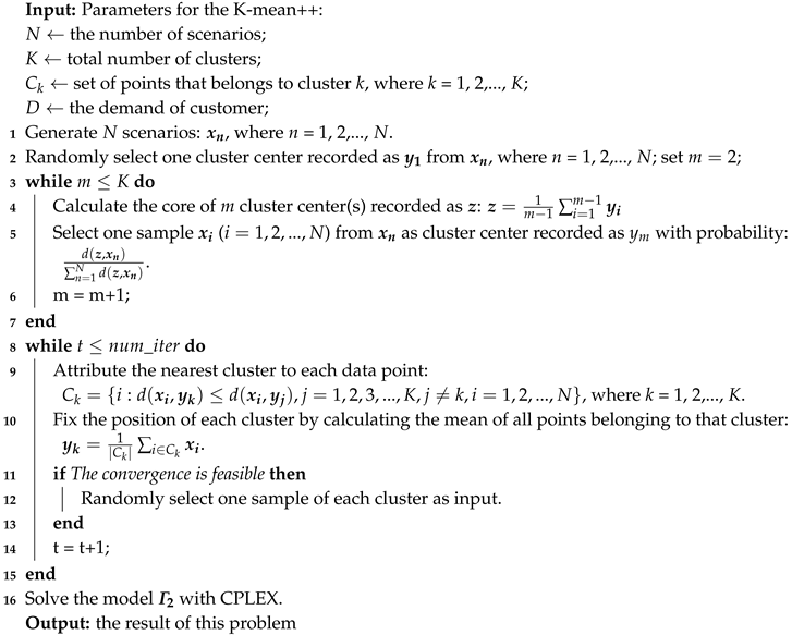
SAA performs well under a large number of samples, but large-scale samples may lead to an increase in the solution time (Emelogu et al. 2016) [18]. Therefore, in this work, we used a clustering (K-means++) algorithm in SAA to dynamically update both sample sizes.

K-means clustering is a popular unsupervised algorithm proposed by Lloyd (1982) [19]. The main idea behind of K-means as flowing is: Firstly, initialed cluster centers are selected randomly and each data point is assigned to one of the clusters by distance. Secondly, the core position of each cluster is updated, and data points are reassigned accordingly. This step is repeated until the convergence requirement is satisfied. However, K-means is also a time consumption.Therefore, K-means++ was proposed by Bahmani et al. (2012) [20] based on K-means. The major difference between K-means++ and K-means is that in the K-means++ algorithm, cluster centers are selected with some probability, which is ensured by the distances between data points and the core of cluster centers. The detail of ESAA is presented in Algorithm 1.

Algorithm 1: Enhanced Sample Average Approximation.

4.3. Markov Approximation (MA)

To achieve an efficient solution quality of the problem, both SAA and ESAA approaches need lots of scenarios. However, solving a large number of scenarios is very time-consuming and not representative of reality. Below, we introduce an approach to Markov approximation, which only requires empirical mean and variance.

Theorem 1.

(REFER TO NG 2014) In Formula (50), $g(·)$ is a definition function. The chance constraint (Equation (14)) is equivalent to Equation (49) as for ${\nu }_{nt}$ given by Equation (51) [21]:

$$P\{\left|X\right|\ge a\}\le \frac{E\left(X\right)}{a},$$

(48)

$$\sum _m{Q}_{mnt}^{SC}\ge {\mu }_{nt}+{\nu }_{nt}n\in N,t\in T,$$

(49)

$$g\left({\nu }_{nt}\right)\equiv \underset{\lambda >0}{min}\left(e^{-\lambda {\nu }_{nt}/{\mu }_{nt}}(1+\frac{{\Sigma }_s}{{\mu }_s^2{\kappa }_{nt}^2}(e^{\lambda {\kappa }_{nt}}-\lambda {\kappa }_{nt}-1))-{\alpha }_{nt}\right)n\in N,t\in T,$$

(50)

$$g\left({\nu }_{nt}\right)=0n\in N,t\in T,$$

(51)

where ${\Sigma }_{nt}$ and ${\mu }_{nt}$ are the empirical mean and variance, and λ is a positive number. ${\xi }_{nt}$ is a random variable to model the deviations from the mean demand of customer n in period t. Then, we can use ${\xi }_{nt}$ and ${\mu }_{nt}$ to denote $D_{nt}$, that is, $D_{nt}={\mu }_{nt}(1+{\xi }_{nt})$. ${\kappa }_{nt}$ is a positive real number such that ${\xi }_{nt}\le {\kappa }_{nt}$.

Markov formulation [${\Gamma }_{\mathbf{3}}$]:

$$\begin{array}{c}maxF\\ s.t.\left(2\right)–\left(13\right),\left(15\right)–\left(46\right),\left(49\right)–\left(51\right)\end{array}$$

4.4. Mixed Integer Second-Order Conic Program (MI-SOCP)

Similarly, another popular approximation approach called mixed integer second-order conic program was adopted in our problem. We approximated the set of unknown distribution by adopting an ambiguity set $D_{nt}^M$ (Delage et al. 2010) [14] to characterize probability $Pr\left(D_{nt}\right)$ for each $n\in N$, $t\in T$. The values of ${\mu }_{nt}^0$ and ${\Sigma }_{nt}^0$ are empirical mean and variance of demand. ${\gamma }_1$ and ${\gamma }_2$ are scalars (${\gamma }_2\ge {\gamma }_1\ge 0$) which are used to adjust the size of ${\mathcal{D}}_{nt}^{\mathcal{M}}$.

$${\mathcal{D}}_{nt}^{\mathcal{M}}({\Xi }_{nt},{\mu }_{nt},{\Sigma }_{nt},{\gamma }_1,{\gamma }_2)=\left\{\begin{array}{cc}Pr\left(D_{nt}\right):& \begin{array}{l}\sum _{\omega =1}^{\infty }Pr\left(D_{nt}\left(\omega \right)\right)=1\\ {\mathbb{E}}_{{\mathbb{P}}_{nt}}{[D_{nt}-{\mu }_{nt})}^2]\le {\gamma }_1{\Sigma }_{nt}\\ {\mathbb{E}}_{{\mathbb{P}}_{nt}}{[D_{nt}-{\mu }_{nt}]}^2\le {\gamma }_2{\Sigma }_{nt}\end{array}\end{array}\right\}$$

Theorem 2.

Based on the set $D_{nt}^M$, Equation (14) can be replaced by Equation (52):

$$\sqrt{\frac{1}{1-{\tau }_1-{\tau }_2}}·\left(1+\sqrt{\frac{{\alpha }_{nt}·{\tau }_2}{1-{\alpha }_{nt}}}\right)·\sqrt{{\Sigma }_{nt}}\le \sqrt{\frac{{\alpha }_{nt}}{1-{\alpha }_{nt}}}·\left(\sum _m{Q}_{mnt}^{SC}-{\mu }_{nt}\right)n\in N,t\in T$$

(52)

where ${\tau }_1$, ${\tau }_2$ and ${\gamma }_1$, ${\gamma }_2$ have the following relations in Equation (53).

$${\tau }_1=\frac{{\gamma }_2-2{\gamma }_1-1}{{\gamma }_2-{\gamma }_1}{\tau }_2=\frac{{\gamma }_1}{{\gamma }_2-{\gamma }_1}$$

(53)

The proof follows Theorem 2.2 in Wagner (2008) [13] and Theorem 2 in Zhang et al. (2018) [17]; we omit the details here.

MI-SOCP formulation [${\Gamma }_{\mathbf{4}}$]:

$$\begin{array}{c}maxF\\ s.t.\left(2\right)–\left(13\right),\left(15\right)–\left(46\right),\left(49\right)–\left(51\right)\end{array}$$

5. Computional Experiments and Discussions

In this section, we first compare the performance among the four proposed approaches. Then, we make sensitivity analyses on the parameter of ${\beta }_1$, ${\beta }_2$ and ${\alpha }_{nt}$. All numerical experiments were conducted on a personal computer with Core I7 in 3.60 GHz processor and 32 GB RAM under a Windows 7 operating system using a state-of-the-art linear programming solver, i.e., CPLEX.

5.1. Out-Of-Sample Test

Similarly with Zhang et al. (2018) [17], the out-of-sample test was implemented, and the main idea behind of it as following: (i) For SAA and ESAA, the customer demand is first determined under limited samples and scenarios; (ii) for MA and MI-SOCP, the demand is decided with a given mean vector and covariance matrix. Then, 10,000 scenarios were randomly generated which satisfied the given conditions of customer demand. This can realize the demand of customer data in uncertain situations. Next, demand data were assigned to each customer via the Moore algorithm [22] under the 10,000 scenarios.

The indicator of reliability was applied to evaluate the out-of-sample performance among the four proposed methods. The reliability is defined as the ratio of the number of scenarios with meeting the customer demand to the total number of scenarios.

5.2. Results on Randomly Generated Instances and Discussion

During the numerical experiments, the set of parameter was tested as $T=6,I=2,J=4,K=6,M=8,N=20,E=2$, and the price of products ranged from 120 to 150 with time varying. Other parameter settings can be similar to the case study reported in the recent literature [23]. For the SAA and ESAA approaches, we generated 20 combinations, including samples in {3, 4, 5, 6} and scenarios in {8, 9, 10, 11, 12}. For the MA and MI-SOCP approach, ${\alpha }_{nt}$ varied in {0.05, 0.1, 0.15, 0.2, 0.25, 0.3}. Numerical experiments were conducted to evaluate the performances of different approaches for different parameters. The computational results are reported in

Table 1. Computational results for sample average approximation (SAA).

Comb	Normal		Uniform		Mixed
	Obj	Times (s)	Obj	Times (s)	Obj	Times (s)
3–8	476,883	43.55	477,131	43.85	507,830	44.90
3–9	476,719	48.91	477,782	49.07	503,987	50.16
3–10	475,642	54.76	474,701	55.12	506,194	56.25
3–11	476,760	61.02	477,241	61.38	502,774	61.32
3–12	478,303	67.17	478,664	67.71	505,624	67.32
4–8	719,521	45.14	719,786	45.55	775,181	45.51
4–9	638,298	51.19	634,276	51.51	681,036	51.51
4–10	571,613	57.52	569,650	58.15	611,721	57.57
4–11	520,274	74.17	519,599	64.60	552,719	64.45
4–12	476,824	70.60	476,374	71.12	505,663	71.03
5–8	714,097	47.44	711,709	47.81	774,953	47.91
5–9	638,023	53.93	637,843	54.45	684,437	54.39
5–10	575,494	60.45	574,313	61.18	614,680	60.90
5–11	520,044	67.67	519,243	68.13	553,761	67.87
5–12	475,129	74.64	475,710	75.11	507,013	75.16
6–8	717,707	50.37	716,349	50.84	775,287	51.52
6–9	635,357	57.44	635,440	57.88	683,887	58.01
6–10	572,779	64.75	571,969	65.30	616,486	65.01
6–11	520,012	72.13	519,467	72.39	554,384	72.58
6–12	476,982	79.87	477,482	79.86	508,359	80.56
Average	557,823	60.14	557,237	60	596,299	60.20

,

Table 2. Computational results for enhanced sample average approximation (ESAA).

Comb	Normal		Uniform		Mixed
	Obj	Times (s)	Obj	Times (s)	Obj	Times (s)
3–8	477,316	44.05	475,724	43.98	481,693	43.71
3–9	476,543	49.18	476,119	49.14	484,265	49.04
3–10	472,977	55.21	474,479	55.37	481,325	54.65
3–11	473,271	61.20	477,738	61.51	482,012	60.95
3–12	476,811	67.69	475,332	67.65	482,361	67.22
4–8	711,575	45.48	713,824	45.41	723,550	45.12
4–9	634,367	51.61	633,246	51.44	641,849	51.16
4–10	570,593	57.93	575,180	57.49	576,043	57.26
4–11	521,022	64.29	519,689	64.27	524,420	64.05
4–12	476,893	70.94	476,839	70.85	482,239	70.55
5–8	717,602	47.79	713,359	47.94	724,671	47.59
5–9	638,641	54.30	635,900	54.29	643,577	54.05
5–10	572,668	61.23	572,277	61.35	578,260	60.66
5–11	520,148	67.82	522,155	68.11	527,016	67.53
5–12	475,630	74.75	476,233	75.44	482,732	74.69
6–8	712,574	50.51	716,193	50.74	723,506	50.42
6–9	635,004	57.52	636,097	57.85	644,178	57.43
6–10	571,026	64.77	572,338	65.10	577,135	64.68
6–11	520,986	72.17	518,471	72.59	523,095	71.90
6–12	476,698	79.76	475,235	80.35	481,558	79.94
Average	556,617	59.91	556,821	60.04	563,274	59.63

,

Table 3. SAA reliability.

n	t = 1			t = 2			t = 3			t = 4			t = 5			t = 6
	Normal	Uniform	Mixed	Normal	Uniform	Mixed	Normal	Uniform	Mixed	Normal	Uniform	Mixed	Normal	Uniform	Mixed	Normal	Uniform	Mixed
1	90.80%	92.40%	94.60%	83.80%	79.00%	86.80%	89.20%	91.40%	92.80%	91.60%	93.20%	93.80%	89.80%	86.60%	88.40%	95.00%	99.60%	99.80%
2	94.80%	97.80%	100.00%	95.00%	93.40%	96.00%	90.60%	91.40%	89.80%	95.00%	96.60%	100.00%	90.40%	89.40%	90.20%	95.20%	99.40%	99.60%
3	90.00%	86.60%	89.60%	92.60%	94.40%	98.00%	89.40%	84.80%	79.60%	88.40%	88.60%	88.20%	90.00%	86.20%	84.80%	95.80%	100.00%	100.00%
4	91.60%	93.40%	93.80%	90.60%	91.20%	96.00%	82.80%	83.00%	80.80%	95.40%	96.80%	99.20%	91.60%	86.00%	91.20%	91.40%	87.00%	91.60%
5	86.20%	74.80%	85.40%	91.20%	90.60%	95.20%	92.00%	88.40%	91.40%	91.60%	89.00%	91.40%	90.20%	98.60%	99.00%	96.40%	95.40%	100.00%
6	84.60%	78.00%	81.40%	94.00%	95.80%	98.20%	94.40%	98.60%	100.00%	87.20%	85.60%	83.80%	94.60%	97.80%	97.60%	88.40%	84.40%	94.80%
7	82.60%	79.60%	83.20%	88.00%	83.40%	85.20%	91.80%	92.20%	93.20%	92.20%	91.00%	93.80%	89.00%	84.60%	91.00%	93.00%	84.80%	92.80%
8	83.60%	77.60%	74.20%	91.80%	80.00%	83.20%	85.60%	85.40%	91.60%	88.40%	87.80%	88.00%	92.40%	94.60%	96.00%	93.60%	88.60%	89.40%
9	89.60%	89.60%	91.80%	88.60%	82.00%	82.80%	85.60%	84.20%	87.20%	91.00%	88.00%	92.60%	91.20%	83.20%	89.80%	90.80%	91.80%	93.40%
10	86.20%	87.60%	86.80%	96.20%	100.00%	100.00%	89.80%	85.60%	90.20%	88.20%	82.40%	88.00%	89.40%	90.80%	93.40%	89.80%	88.80%	88.00%
11	82.80%	84.00%	84.00%	92.00%	90.60%	90.80%	87.60%	83.40%	85.80%	89.60%	85.20%	91.40%	92.40%	87.80%	90.20%	93.00%	93.00%	98.20%
12	84.40%	77.40%	79.00%	80.40%	75.80%	78.20%	86.80%	81.00%	78.80%	96.60%	100.00%	100.00%	87.80%	81.60%	86.80%	92.40%	91.20%	93.60%
13	81.80%	81.40%	83.40%	85.40%	84.60%	82.20%	88.20%	80.40%	83.00%	87.00%	79.40%	88.60%	97.00%	100.00%	100.00%	92.80%	89.60%	95.60%
14	93.40%	95.00%	92.20%	95.20%	91.20%	94.20%	92.80%	89.20%	96.00%	91.60%	89.00%	85.60%	94.60%	100.00%	100.00%	95.80%	97.80%	100.00%
15	86.20%	74.00%	79.80%	84.00%	85.20%	92.80%	87.20%	85.20%	87.40%	87.00%	83.20%	79.20%	92.60%	98.00%	99.00%	90.60%	88.80%	95.00%
16	87.80%	85.80%	88.80%	84.80%	86.20%	83.80%	84.40%	83.40%	80.20%	86.20%	84.20%	80.60%	90.60%	91.60%	91.80%	92.80%	94.40%	92.00%
17	85.20%	79.60%	81.00%	93.60%	93.40%	97.80%	87.40%	91.60%	93.40%	96.80%	100.00%	100.00%	98.80%	100.00%	100.00%	97.60%	100.00%	100.00%
18	88.40%	83.80%	83.00%	88.00%	88.20%	87.20%	89.60%	91.40%	92.60%	93.00%	92.20%	95.20%	89.00%	87.80%	91.20%	93.40%	91.80%	93.80%
19	80.00%	76.40%	78.20%	82.00%	72.60%	75.20%	91.80%	92.00%	96.40%	89.40%	86.60%	85.20%	85.20%	82.60%	90.60%	95.60%	92.20%	97.00%
20	85.80%	78.00%	80.80%	86.40%	78.00%	80.00%	92.80%	88.80%	94.40%	88.00%	85.00%	86.40%	96.80%	100.00%	100.00%	89.60%	90.00%	85.60%
Average	86.79%	83.64%	85.55%	89.18%	86.78%	89.18%	88.99%	87.57%	89.23%	90.71%	89.19%	90.55%	91.67%	91.36%	93.55%	93.15%	92.43%	95.01%

,

Table 4. ESAA reliability.

n	t = 1			t = 2			t = 3			t = 4			t = 5			t = 6
	Normal	Uniform	Mixed	Normal	Uniform	Mixed	Normal	Uniform	Mixed	Normal	Uniform	Mixed	Normal	Uniform	Mixed	Normal	Uniform	Mixed
1	91.34%	88.81%	97.27%	87.95%	84.26%	94.43%	92.19%	92.27%	97.92%	91.17%	91.88%	97.01%	90.02%	87.51%	96.07%	96.83%	100.00%	98.79%
2	92.98%	91.98%	98.09%	95.11%	99.91%	98.33%	92.09%	88.05%	96.78%	94.23%	93.91%	98.24%	93.13%	91.39%	96.81%	95.60%	100.00%	98.34%
3	91.84%	89.92%	96.70%	92.59%	91.49%	97.66%	87.03%	84.85%	95.44%	89.23%	88.70%	96.66%	88.64%	85.12%	94.69%	96.24%	100.00%	98.70%
4	91.65%	88.97%	96.83%	92.45%	89.42%	97.58%	86.71%	80.42%	93.29%	94.63%	95.71%	98.21%	90.27%	87.65%	96.74%	89.58%	90.88%	96.32%
5	81.39%	75.52%	89.10%	92.14%	87.53%	97.08%	89.91%	88.82%	96.42%	91.05%	88.31%	96.90%	95.38%	94.66%	98.15%	94.89%	96.41%	98.46%
6	85.41%	79.22%	95.80%	93.74%	93.46%	98.47%	96.66%	99.49%	98.72%	89.69%	85.62%	96.55%	92.53%	97.45%	97.78%	88.46%	85.32%	96.45%
7	86.64%	81.47%	91.10%	90.07%	85.61%	95.79%	92.42%	91.15%	97.17%	91.71%	93.01%	98.04%	93.49%	91.49%	96.99%	93.72%	94.17%	97.54%
8	79.93%	75.07%	88.38%	84.20%	82.20%	93.15%	88.81%	88.66%	96.02%	89.41%	87.09%	95.71%	94.35%	91.41%	97.65%	91.01%	85.48%	97.13%
9	89.49%	86.18%	96.94%	86.37%	82.04%	95.20%	86.07%	83.87%	95.72%	91.20%	90.91%	97.07%	89.20%	84.60%	95.93%	91.44%	92.36%	97.96%
10	88.64%	87.36%	95.10%	95.65%	100.00%	98.57%	90.57%	86.85%	96.90%	85.10%	82.28%	95.64%	91.53%	88.80%	96.76%	91.21%	86.14%	97.05%
11	83.54%	78.60%	94.56%	90.50%	89.27%	97.21%	88.92%	83.59%	96.01%	91.26%	85.51%	96.32%	92.81%	87.06%	95.59%	93.40%	97.83%	97.71%
12	83.88%	78.18%	85.19%	84.24%	76.22%	89.44%	86.95%	81.03%	91.87%	96.11%	100.00%	98.71%	86.44%	85.03%	94.54%	91.95%	93.86%	97.74%
13	87.79%	84.98%	93.23%	86.11%	80.91%	93.49%	86.82%	83.32%	93.93%	88.12%	82.26%	95.30%	96.55%	100.00%	99.05%	91.33%	88.27%	97.34%
14	95.29%	95.73%	97.61%	92.80%	91.28%	97.94%	92.42%	91.20%	97.25%	89.26%	84.88%	95.15%	95.38%	100.00%	98.82%	94.59%	97.85%	98.31%
15	81.96%	75.16%	87.24%	88.06%	84.81%	94.04%	88.17%	88.70%	95.86%	85.99%	78.12%	94.00%	94.36%	94.37%	98.07%	90.78%	90.03%	97.05%
16	89.99%	86.80%	94.56%	87.52%	80.32%	91.31%	86.74%	79.71%	94.93%	85.77%	79.20%	90.28%	92.22%	87.23%	96.18%	93.01%	90.07%	97.03%
17	84.76%	81.62%	92.94%	93.03%	96.13%	98.14%	90.25%	85.88%	96.45%	96.94%	100.00%	99.17%	97.79%	100.00%	99.19%	97.98%	100.00%	99.37%
18	87.07%	80.88%	94.98%	88.72%	82.06%	95.60%	92.92%	93.67%	97.64%	92.62%	94.91%	97.57%	91.99%	89.80%	95.84%	90.89%	95.59%	97.30%
19	80.98%	77.42%	87.72%	80.34%	73.59%	84.38%	92.01%	90.94%	97.35%	90.93%	87.80%	96.12%	90.14%	85.11%	96.13%	93.21%	91.94%	97.72%
20	85.54%	79.33%	88.98%	85.51%	78.42%	92.89%	91.85%	89.95%	98.03%	92.19%	83.29%	96.24%	97.08%	100.00%	99.10%	89.06%	85.89%	96.12%
Average	87.01%	83.16%	93.12%	89.36%	86.45%	95.04%	89.98%	87.62%	96.19%	90.83%	88.67%	96.44%	92.67%	91.43%	97.00%	92.76%	93.10%	97.62%

and

Table 5. Mixed integer second-order conic program (MISOCP) reliability.

n	t = 1			t = 2			t = 3			t = 4			t = 5			t = 6
	$\mathit{\alpha }$ = 0.05	$\mathit{\alpha }$ = 0.1	$\mathit{\alpha }$= 0.15	$\mathit{\alpha }$ = 0.05	$\mathit{\alpha }$ = 0.1	$\mathit{\alpha }$ = 0.05	$\mathit{\alpha }$ = 0.05	$\mathit{\alpha }$ = 0.1	$\mathit{\alpha }$ = 0.15	$\mathit{\alpha }$ = 0.05	$\mathit{\alpha }$ = 0.1	$\mathit{\alpha }$ = 0.05	$\mathit{\alpha }$ = 0.05	$\mathit{\alpha }$= 0.1	$\mathit{\alpha }$ = 0.15	$\mathit{\alpha }$= 0.05	$\mathit{\alpha }$ = 0.1	$\mathit{\alpha }$ = 0.15
1	69.69%	58.21%	53.00%	100.00%	95.99%	90.19%	100.00%	98.00%	92.19%	100.00%	100.00%	100.00%	100.00%	100.00%	100.00%	100.00%	100.00%	100.00%
2	100.00%	90.22%	83.91%	100.00%	100.00%	100.00%	100.00%	100.00%	100.00%	100.00%	100.00%	100.00%	100.00%	100.00%	100.00%	100.00%	100.00%	100.00%
3	60.91%	49.10%	44.91%	88.57%	78.80%	72.65%	100.00%	97.19%	90.37%	100.00%	100.00%	100.00%	100.00%	100.00%	100.00%	100.00%	100.00%	100.00%
4	99.05%	85.97%	80.83%	99.14%	87.26%	81.24%	100.00%	100.00%	100.00%	100.00%	91.07%	86.23%	100.00%	100.00%	100.00%	100.00%	100.00%	100.00%
5	93.99%	77.61%	68.45%	71.15%	59.98%	54.09%	79.50%	67.15%	60.71%	96.13%	83.15%	76.87%	100.00%	100.00%	100.00%	100.00%	100.00%	100.00%
6	88.58%	73.15%	67.21%	100.00%	96.07%	90.68%	100.00%	100.00%	97.05%	100.00%	100.00%	100.00%	100.00%	100.00%	100.00%	100.00%	100.00%	100.00%
7	79.51%	65.34%	60.12%	75.69%	63.49%	57.31%	80.18%	68.40%	62.58%	100.00%	97.10%	90.91%	100.00%	100.00%	100.00%	100.00%	100.00%	100.00%
8	91.19%	74.56%	67.44%	100.00%	96.89%	89.72%	100.00%	96.90%	89.99%	100.00%	100.00%	100.00%	100.00%	100.00%	100.00%	100.00%	100.00%	100.00%
9	81.40%	68.66%	63.13%	100.00%	94.33%	87.25%	100.00%	100.00%	98.92%	100.00%	100.00%	100.00%	100.00%	100.00%	100.00%	100.00%	100.00%	100.00%
10	82.71%	70.59%	64.35%	100.00%	100.00%	96.71%	100.00%	100.00%	100.00%	100.00%	100.00%	100.00%	100.00%	100.00%	100.00%	100.00%	100.00%	100.00%
11	81.13%	66.02%	59.34%	71.54%	59.63%	54.17%	82.05%	68.49%	63.29%	85.90%	73.75%	67.41%	100.00%	100.00%	95.76%	100.00%	100.00%	100.00%
12	100.00%	88.05%	80.35%	100.00%	88.36%	80.36%	100.00%	100.00%	100.00%	100.00%	100.00%	100.00%	100.00%	100.00%	100.00%	100.00%	100.00%	100.00%
13	94.03%	79.61%	72.39%	100.00%	85.31%	79.13%	100.00%	86.59%	79.34%	100.00%	100.00%	100.00%	100.00%	100.00%	100.00%	100.00%	100.00%	100.00%
14	85.64%	74.85%	68.91%	100.00%	100.00%	100.00%	100.00%	100.00%	100.00%	100.00%	100.00%	100.00%	100.00%	100.00%	100.00%	100.00%	100.00%	100.00%
15	89.44%	72.59%	64.86%	75.87%	62.32%	56.35%	100.00%	100.00%	97.91%	100.00%	100.00%	100.00%	100.00%	100.00%	96.16%	100.00%	100.00%	100.00%
16	72.00%	60.41%	53.99%	100.00%	84.74%	79.15%	100.00%	92.51%	85.01%	100.00%	100.00%	96.92%	100.00%	100.00%	100.00%	100.00%	100.00%	100.00%
17	100.00%	100.00%	100.00%	100.00%	100.00%	100.00%	100.00%	100.00%	100.00%	100.00%	100.00%	100.00%	100.00%	100.00%	100.00%	100.00%	100.00%	100.00%
18	87.96%	73.88%	68.66%	100.00%	100.00%	93.03%	100.00%	100.00%	100.00%	100.00%	100.00%	100.00%	100.00%	100.00%	100.00%	100.00%	100.00%	100.00%
19	90.26%	71.88%	64.61%	92.98%	75.77%	68.11%	75.29%	63.42%	59.71%	100.00%	100.00%	100.00%	100.00%	100.00%	100.00%	100.00%	100.00%	100.00%
20	97.03%	81.11%	73.79%	100.00%	92.15%	84.06%	100.00%	100.00%	100.00%	100.00%	100.00%	100.00%	100.00%	100.00%	100.00%	100.00%	100.00%	100.00%
Average	87.23%	74.09%	68.01%	93.75%	86.05%	80.71%	95.85%	91.93%	88.85%	99.10%	97.25%	95.92%	100.00%	100.00%	99.60%	100.00%	100.00%	100.00%

, and the discussion is shown in Figure 2, Figure 3, Figure 4, Figure 5 and Figure 6.

5.2.1. Performance of the Four Proposed Approaches

The computational results of SAA and ESAA under different samples and scenarios are shown in Table 1 and Table 2. In the tables, the first column denotes different combinations (e.g., ‘3–8’ means 3 samples and 8 scenarios). Additionally, the second column to the fourth represent the different distribution types of customer demand (i.e., normal, uniform, and mix of normal and uniform). We can observe in the two tables that solution qualities of the SAA and ESAA are roughly the same. As for running time, ESAA consumes less time than SAA. However, for a large scale of samples or scenarios, both SAA and ESAA approaches generally consume a long time to get the solution.

The out-of-sample reliability performance is the quality reaction of solutions. From Table 3 and Table 4, the average reliability of all experiment results for ESAA is 91.22%, and for SAA it is 89.38%, which indicates that ESAA can obtain a higher quality than SAA. For the results of the MA and MI-SOCP approaches in Table 5 and

Table 6. Markov approximation (MA) reliability.

n	t = 1			t = 2			t = 3			t = 4			t = 5			t = 6
	$\mathit{\alpha }$ = 0.05	$\mathit{\alpha }$ = 0.1	$\mathit{\alpha }$= 0.15	$\mathit{\alpha }$ = 0.05	$\mathit{\alpha }$ = 0.1	$\mathit{\alpha }$ = 0.05	$\mathit{\alpha }$ = 0.05	$\mathit{\alpha }$ = 0.1	$\mathit{\alpha }$ = 0.15	$\mathit{\alpha }$ = 0.05	$\mathit{\alpha }$ = 0.1	$\mathit{\alpha }$ = 0.05	$\mathit{\alpha }$ = 0.05	$\mathit{\alpha }$= 0.1	$\mathit{\alpha }$ = 0.15	$\mathit{\alpha }$= 0.05	$\mathit{\alpha }$ = 0.1	$\mathit{\alpha }$ = 0.15
1	100.00%	100.00%	93.69%	100.00%	100.00%	100.00%	100.00%	100.00%	100.00%	100.00%	100.00%	100.00%	100.00%	100.00%	100.00%	100.00%	100.00%	100.00%
2	100.00%	100.00%	100.00%	100.00%	100.00%	100.00%	100.00%	100.00%	100.00%	100.00%	100.00%	100.00%	100.00%	100.00%	100.00%	100.00%	100.00%	100.00%
3	100.00%	90.17%	80.73%	100.00%	100.00%	100.00%	100.00%	100.00%	100.00%	100.00%	100.00%	100.00%	100.00%	100.00%	100.00%	100.00%	100.00%	100.00%
4	100.00%	100.00%	100.00%	100.00%	100.00%	100.00%	100.00%	100.00%	100.00%	100.00%	100.00%	100.00%	100.00%	100.00%	100.00%	100.00%	100.00%	100.00%
5	100.00%	97.13%	86.83%	100.00%	100.00%	94.28%	100.00%	100.00%	96.98%	100.00%	100.00%	100.00%	100.00%	100.00%	100.00%	100.00%	100.00%	100.00%
6	100.00%	100.00%	90.31%	100.00%	100.00%	100.00%	100.00%	100.00%	100.00%	100.00%	100.00%	100.00%	100.00%	100.00%	100.00%	100.00%	100.00%	100.00%
7	100.00%	95.01%	79.86%	100.00%	100.00%	91.97%	100.00%	100.00%	100.00%	100.00%	100.00%	100.00%	100.00%	100.00%	100.00%	100.00%	100.00%	100.00%
8	100.00%	97.91%	84.25%	100.00%	100.00%	100.00%	100.00%	100.00%	100.00%	100.00%	100.00%	100.00%	100.00%	100.00%	100.00%	100.00%	100.00%	100.00%
9	100.00%	100.00%	100.00%	100.00%	100.00%	100.00%	100.00%	100.00%	100.00%	100.00%	100.00%	100.00%	100.00%	100.00%	100.00%	100.00%	100.00%	100.00%
10	100.00%	100.00%	98.15%	100.00%	100.00%	100.00%	100.00%	100.00%	100.00%	100.00%	100.00%	100.00%	100.00%	100.00%	100.00%	100.00%	100.00%	100.00%
11	100.00%	94.85%	79.39%	100.00%	100.00%	90.19%	100.00%	100.00%	95.15%	100.00%	100.00%	100.00%	100.00%	100.00%	100.00%	100.00%	100.00%	100.00%
12	100.00%	100.00%	98.06%	100.00%	100.00%	98.19%	100.00%	100.00%	100.00%	100.00%	100.00%	100.00%	100.00%	100.00%	100.00%	100.00%	100.00%	100.00%
13	100.00%	100.00%	96.89%	100.00%	100.00%	100.00%	100.00%	100.00%	100.00%	100.00%	100.00%	100.00%	100.00%	100.00%	100.00%	100.00%	100.00%	100.00%
14	100.00%	100.00%	100.00%	100.00%	100.00%	100.00%	100.00%	100.00%	100.00%	100.00%	100.00%	100.00%	100.00%	100.00%	100.00%	100.00%	100.00%	100.00%
15	100.00%	92.91%	83.13%	100.00%	100.00%	88.54%	100.00%	100.00%	100.00%	100.00%	100.00%	100.00%	100.00%	100.00%	100.00%	100.00%	100.00%	100.00%
16	100.00%	97.17%	87.53%	100.00%	100.00%	100.00%	100.00%	100.00%	100.00%	100.00%	100.00%	100.00%	100.00%	100.00%	100.00%	100.00%	100.00%	100.00%
17	100.00%	100.00%	100.00%	100.00%	100.00%	100.00%	100.00%	100.00%	100.00%	100.00%	100.00%	100.00%	100.00%	100.00%	100.00%	100.00%	100.00%	100.00%
18	100.00%	100.00%	97.05%	100.00%	100.00%	100.00%	100.00%	100.00%	100.00%	100.00%	100.00%	100.00%	100.00%	100.00%	100.00%	100.00%	100.00%	100.00%
19	100.00%	89.67%	79.33%	100.00%	95.14%	79.06%	100.00%	100.00%	96.95%	100.00%	100.00%	100.00%	100.00%	100.00%	100.00%	100.00%	100.00%	100.00%
20	100.00%	100.00%	93.76%	100.00%	100.00%	100.00%	100.00%	100.00%	100.00%	100.00%	100.00%	100.00%	100.00%	100.00%	100.00%	100.00%	100.00%	100.00%
Average	100.00%	97.74%	91.45%	100.00%	99.76%	97.11%	100.00%	100.00%	99.45%	100.00%	100.00%	100.00%	100.00%	100.00%	100.00%	100.00%	100.00%	100.00%

, we can get that the average reliability of all instances is 99.20% and 92.13%, respectively.

However, the reliabilities of the MI-SOCP approaches cannot meet the given risk level ${\alpha }_{nt}$ in some period t. To make that a little more clear, take ${\alpha }_{nt}=0.05$ as an example. When ${\alpha }_{nt}=0.05$, it means that the reliability is no less than 95% in $n\in N,t\in T$. However, the mean reliability of MI-SOP is 87.23% in period $t=1$, which is smaller than 95%. By contrast, the approach of MA can achieve very high reliabilities under all conditions of risk ${\alpha }_{nt}$. Therefore, in sum, the approach of MA can get the best solution among the four proposed approaches.

5.2.2. Impact of the Combination of ${\beta }_1$, ${\beta }_2$ and ${\alpha }_{nt}$

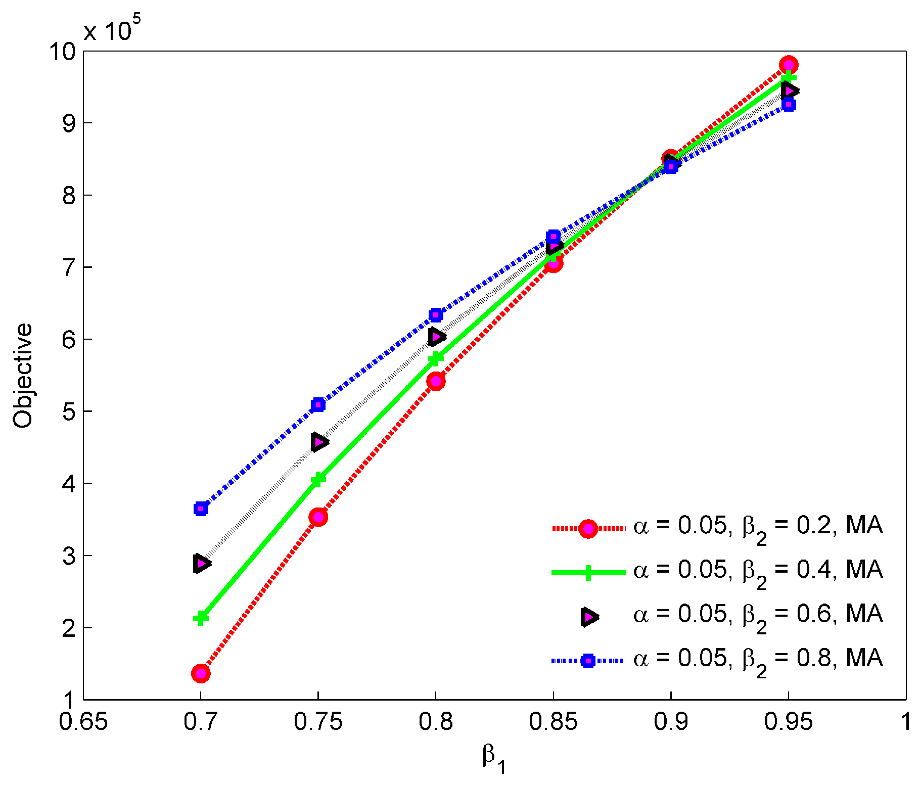
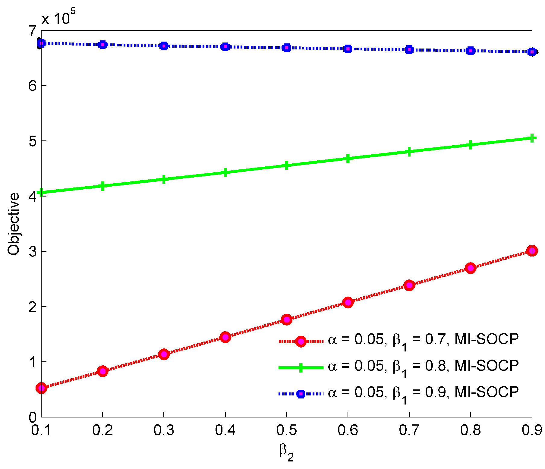
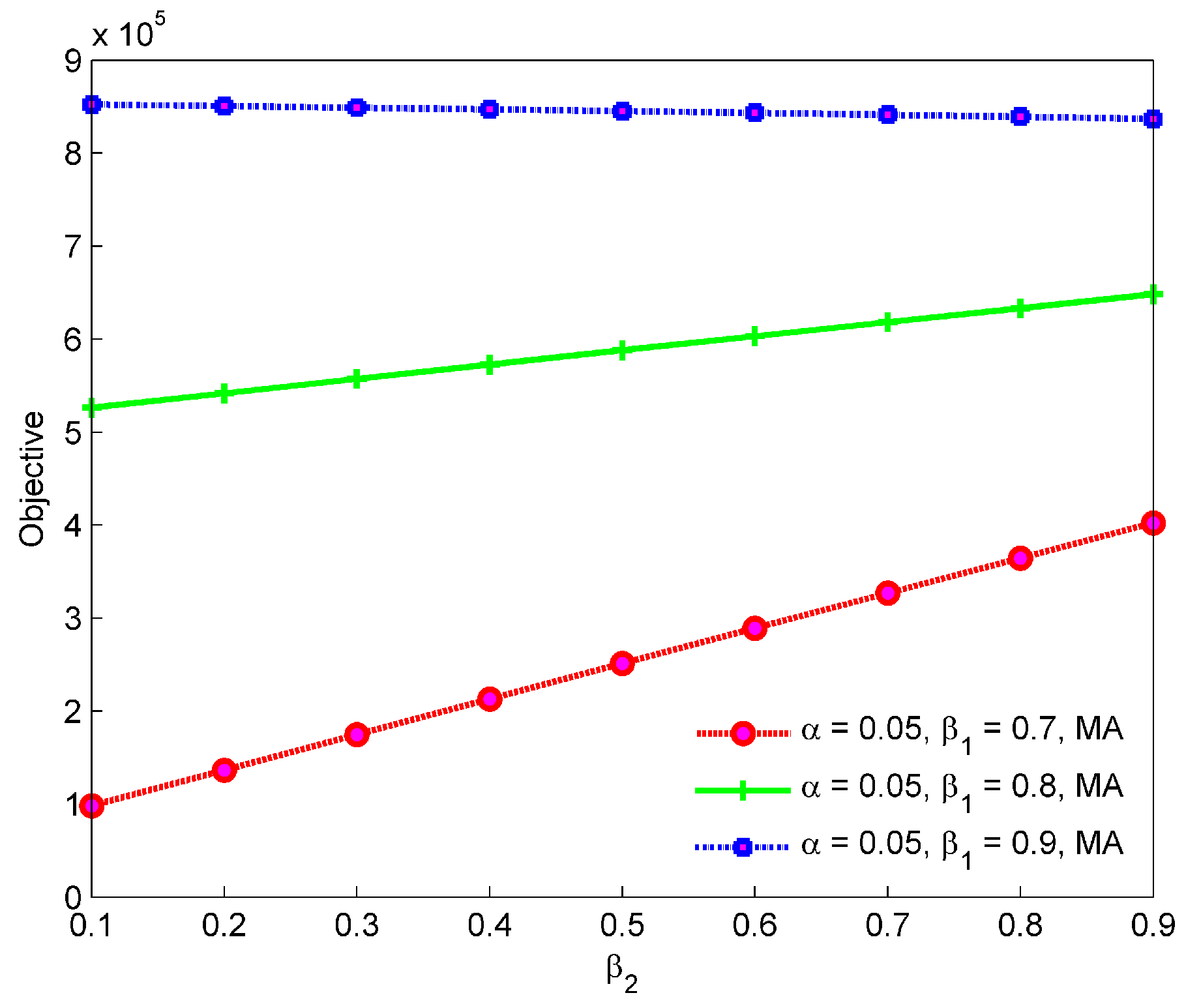
In order to analyze the importance of parameter $bet{a}_1$ in our objective, computational experiments under ${\alpha }_{nt}=0.05$ with ${\beta }_2=\{0.2,0.4,0.6,0.8\}$ were conducted in the MA and MI-SOCP approaches. Figure 2 and Figure 3 show that the MA solution approach performed better than MI-SOCP, which is consistent with the abovementioned. Increasing with ${\beta }_1$, the firm can obtain a huge profit under the fixed ${\beta }_2$ and ${\alpha }_{nt}$ value. This implies that the firm needs to improve the conversion rate of raw materials, such as using new technologies or equipment. By testing the parameter combinations of ${\beta }_2$, Figure 2 and Figure 3 illustrate that a higher ${\beta }_1$ and ${\beta }_2$ combination cannot get the optimal objective value. The firm can dynamically adjust the raw materials conversion ratio and recycling rate to realize profit maximization. An interesting thing to note is that the recycling rate of products ${\beta }_2$ can influence profit. Figure 4 and Figure 5 display that with a fixed ${\beta }_1$, a high ratio of ${\beta }_2$ can achieve high profit. However, when the ${\beta }_1$ increases with a high value (e.g., ${\beta }_1$ = 0.8), it cannot help to improve the profit of the firm. 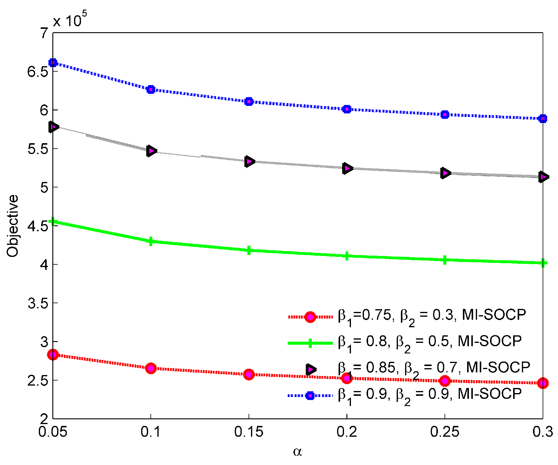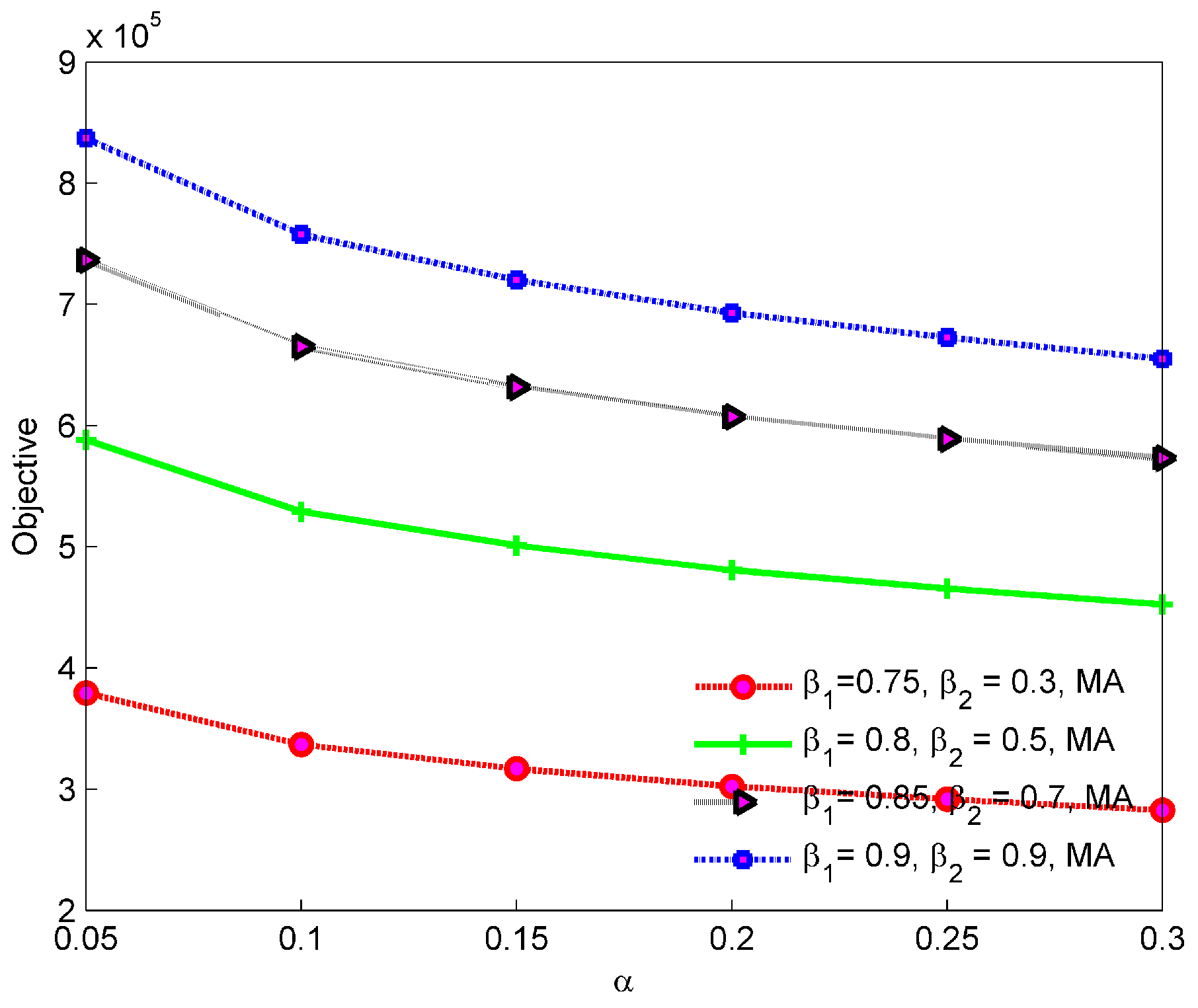As for the risk level ${\alpha }_{nt}$, we randomly selected four combinations of ${\beta }_1$ and ${\beta }_2$. Figure 6 and Figure 7 illustrate that low risk level can help the firm to get more profit, and the firm needs to take some measures to meet customer demand. The contrast between the approaches of MA and MI-SOCP can be seen again in Figure 2, Figure 3, Figure 4, Figure 5, Figure 6 and Figure 7 which verifies the effectiveness of the MA approach.

6. Conclusions

In this work, we studied a closed-loop supply chain problem considering finance under uncertain customer demand. To the best of our knowledge, we are the first to take into account finance in a closed-loop supply chain and uncertain customer demand simultaneously. We first applied an ambiguity set with empirical mean and variance to portray the demand uncertainty. Moreover, a joint chance constraint programming model was proposed to maximize total profit considering the overproduction penalty cost. Four distribution-free approximation approaches were proposed to solve this stochastic problem. Numerical experiments were conducted to evaluate the performance of our proposed methods, and computational results showed that the Markov approximation approach can obtain higher profit with less computation time. Finally, we conducted an experiment with different parameter combinations and made sensitivity analyses. The results revealed: (i) Markov approximation is more efficient than MI-SOCP, and the objective value increases with the ${\alpha }_{nt}$ increasing when ${\beta }_2$ is fixed; (ii) the recycling rate of products ${\beta }_2$ can influence profit. A higher ${\beta }_2$ value can help the firm to obtain more profit under the same ${\alpha }_{nt}$. However, the relationship between ${\beta }_1$ and ${\beta }_2$ becomes weak when the ${\beta }_1$ value is high and (iii) the objective value decreases when the risk level ${\alpha }_{nt}$ is increasing. The results can help closed-loop supply chain companies to: (i) Balance the relationship between material flow and financial flow and (ii) make more reasonable production scheduling with customer demand uncertainty.

Future research directions may include the following two issues:

• The supply chain financial problem is usually complicated, involving material flow, information flow, and fund flow. Factors such as information can be further considered in the mathematical model. Moreover, various types of financial resources can be applied in the model, including bank credit, capital budget, and securities transactions.
• In order to solve the large scal problem more efficiently, meta-heuristics need to be proposed. Additionally, to improve the solution of the SOCP problem with high accuracy, more approximation approaches need to be designed.