Comparison of CO₂ emissions reduction efficiency of household fuel consumption in China

Abstract

The purpose of this paper is to analyze the correlations among per capita gross domestic product (GDP), household fuel (natural gas and liquefied petroleum gas) consumption, and carbon dioxide (CO₂) emissions through the environmental Kuznets curve (EKC) at the regional and national level in China using data from 2003 to 2015. The results validate the EKC assumption and show that per capita GDP is positively related to CO₂ emissions; per capita natural gas consumption has a negative impact on CO₂ emissions; however, per capita liquefied petroleum gas (LPG) consumption has a positive effect on CO₂ emissions. Therefore, increasing natural gas consumption can effectively slow down the environmental degradation of China. Given rapid economic growth, changing the energy structure can improve the environment.

1. Introduction

In recent years, with sustained economic growth, the attention paid to environmental deterioration is obvious. However, natural resource consumption contributes to economic growth and social progress. If the relationship between natural resources and economic growth is not coordinated, the environment will deteriorate. [1] Such problems are common in countries such as China, and the relationship between economic growth and energy consumption is also important. In China, economic growth has been accompanied by negative effects such as severe depletion of natural resources, environmental pollution, and increased CO₂ emissions. In particular, energy consumption has increased dramatically over the last three decades and led to a sharp growth in China’s gross domestic product (GDP). However, China’s economic development has caused many environmental problems, especially CO₂ emissions [2] According to China Emission Accounts and Datasets (CEADs), CO₂ emissions totaled about 137.31 million tons (Mt) in 1997 and 318.55 million tons (Mt) in 2015, more than twofold increase. With the rapid growth of energy consumption, energy protection policies have become particularly important in China. Therefore, estimating the intensity of energy consumption and the substitution of clean energy is of great significance to environmental protection decisions.

In the late 1980s, though natural gas was able to replace most liquefied petroleum gas, a large number of urban residents began to use liquefied petroleum gas until the beginning of the twenty-first century. Recently, natural gas has been used in greater amounts, and the use of liquefied petroleum gas has declined. Natural gas consumption directly affects the share of liquefied petroleum gas and coal gas due to its lower price, its being more efficient, and its being cleaner for the environment than liquefied petroleum gas. However, natural gas cannot replace liquefied petroleum gas in the short term. Since pipeline natural gas is not available in all areas, and the supporting cost is expensive, suburbs and remote towns still use bottled liquefied petroleum gas because they have no pipeline natural gas. In addition, the operating temperature and characteristics of liquefied petroleum gas determine that it cannot be completely replaced by natural gas in certain special conditions such as welding and cutting. At present, as one of the most widely used clean energy sources, natural gas has received strong support from the country in civilian applications and will replace most liquefied petroleum gas, but both will be used in their fields to replace coal gas.

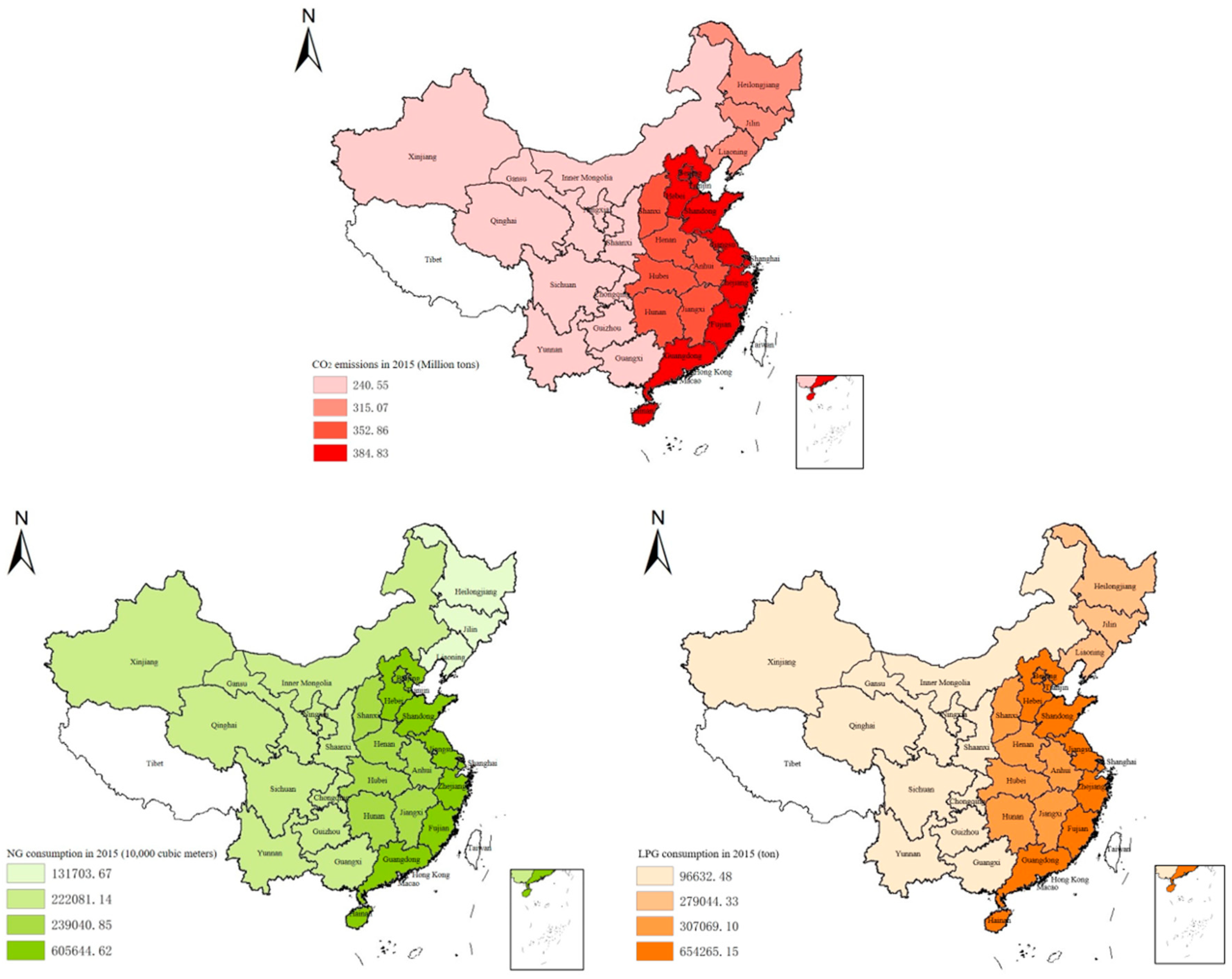
However, natural gas and liquefied petroleum gas consumption contribute to most of the CO₂ emissions in China. Even so, due to the extremely uneven distribution of population and energy in China, there is a big difference between energy consumption in the eastern, central, western, and northeastern regions of China. As depicted in Figure 1, natural gas consumption is much higher in the eastern than in the central, western, and northeastern regions. More specifically, in 2015, the ratios of CO₂ emissions were 30%, 27%, 19%, 24% in the eastern, central, western, and northeastern regions, respectively. The proportions of natural gas consumption were 50%, 20%, 18%, 12% in the eastern, central, western, and northeastern regions, respectively. The ratios of liquefied petroleum gas consumption were 49%, 23%, 7%, 21% in the eastern, central, western, and northeastern regions, respectively. The above facts show that CO₂ emissions and liquefied petroleum gas consumption decrease from the eastern region to the central region to the northeast region to the western region. Due to the abundant natural gas reserves in western China, natural gas consumption decreases from the eastern to the central to the western to the northeast regions. The four regions have a huge difference in energy intensity. This means that estimating the energy consumption in the four regions of China is important for environmental protection, which plays a guiding role in the formulation of policies to reduce energy consumption and promote clean energy use in China and the four regions.

Based on this background, to the best of our knowledge, previous literatures have analyzed the dynamic relationship between CO₂ emissions, economic growth, and energy intensity and consumption limited to coal. [3,4,5,6] The objective of this study is to be the first attempt to investigate the relationships between CO₂ emissions, economic growth, and household fuel (natural gas and liquefied petroleum gas) consumption using an “inverted U-shaped” environmental Kuznets curve (EKC) model for a panel of 30 provinces in China, and to be the first to add household fuel (natural gas and liquefied petroleum gas) consumption as a new explanatory variable to study the effects of household fuel consumption on CO₂ emissions, which can fill the knowledge gap for the nexus of selected variables.

The remaining sections are structured as follows. Section 2 reviews the relevant literature. Section 3 presents the model, data, and estimation methods. Section 4 discusses the empirical results. The final section offers the conclusions and policy implications.

2. Literature Review

CO₂ is an important atmospheric gas that causes global warming. Hence, this study examines the causal relation between CO₂ emissions and economic growth through the environmental Kuznets curve. Previous studies have found an inverted U-shaped relationship exists between CO₂ emissions and economic growth. This can be explained by the fact that pollution increases with GDP growth. When income reaches a “turning point,” the environmental quality improves. In other words, this relationship can be explained by an economic theory that is a kind of income effect. As the economy develops, consumers reach higher levels of consumption and begin to demand increased investment in environmental protection. This point is called the “return point of income.” After the turning point, income continues to increase and environmental quality begins to improve. Since the introduction of the environmental Kuznets curve by Grossman and Krueger [7], the relation between environmental pollution and economic growth has been a popular topic in economic research and has certain practical significance for environmental policies.

2.1. The Presence of EKC

On the basis of many studies, the results of research can be roughly divided into two categories. In the first, the EKC is assumed to be present. For example, Shen and Wu [8] selected Beijing as a case city and used the EKC theory to determine the four stages of development in Beijing. Jalil and Mahmud [9] used time series data from 1975 to 2005 to analyze the long-term connections between China’s CO₂ emissions and energy consumption, wages, and overseas business, and disclosed a nexus between wage and CO₂ emissions to support the EKC. Lindmark [10] has explored the inverted U-shaped trajectory of CO₂ emissions in Sweden since 1870. In addition, Heil and Selden [11], Moomaw and Unruh [12], Selden and Song [13], Holtz-Eakin and Selden [14], Sachs et al. [15], and Galeotti et al. [16] have empirically tested the inverted U-shaped nexus between CO₂ emissions and economic growth, proving the existence of the EKC. In the second category, the EKC is assumed to be absent. Lantz and Feng [17] have found no significant nexus between CO₂ emissions and economic growth. Shafik and Bandyopadhyay [18] have shown that CO₂ emissions have a monotonic relationship with economic growth and that there is no inflection point. Moomaw and Unruh [12], Friedl and Getzner [19], and Martínez-Zarzoso and Bengochea-Morancho [20] have found that CO₂ emissions and economic growth have an N-shaped relationship. Despite these differences, these studies indicate that CO₂ emissions will grow as countries implement economic growth policies.

2.2. Energy Consumption and Economic Growth

Energy consumption drives economic growth, increases CO₂ emissions, and results in environmental degradation and global warming. Dong [21] has studied correlations among CO₂ emissions, GDP, natural gas, and renewable energy consumption in BRICS countries (i.e., Brazil, Russia, India, China, and South Africa) from 1985 to 2016. Dong [22] analyzed the potential impact of natural gas consumption on CO₂ emissions using 1995–2014 panel data from 30 provinces in China. Dong [23] also analyzed the nexus between natural gas consumption and CO₂ emissions in 14 Asia-Pacific countries from 1970 to 2016. Feng [24] has investigated long-run equilibrium relationships between energy consumption structures, economic structures, and energy intensity in China. Bhattacharya [25] investigated the effects of renewable energy consumption on the economic growth of 38 top renewable energy consuming countries from 1991 to 2012. Alper et al. [26] have examined the linkages between economic growth and renewable energy consumption for new European Union member countries during the period 1990–2009. Dong [27] has analyzed the effects of natural gas and renewable energy consumption on CO₂ emissions, with results showing that natural gas and renewable energy consumption have a beneficial impact on CO₂ emissions reduction. In addition, Halicioglu [28], Ozturk et al. [29], Acaravci et al. [30], Wang et al. [31], Arouri et al. [32], Pao et al. [33], Hossain [34], and Pao et al. [35] have verified the causality linkage between CO₂ emissions and energy consumption.

According to the literature examined, many scholars have studied the EKC connection between CO₂ emissions and economic growth, as well as the nexus between CO₂ emissions and energy consumption from fossil fuel. However, few articles have included household fuel in models to analyze CO₂ emissions.

3. Model, Methodology, and Data

3.1. Model and Methodology

One objective of this study is to analyze the dynamic relationship between China’s CO₂ emissions, economic growth, and household fuel (natural gas and liquefied petroleum gas) consumption. In addition, we also examine the effectiveness of the EKC. Therefore, following a previous study by Dong [22], this paper extends the EKC model and adds household fuel (natural gas and liquefied petroleum gas) consumption as a new explanatory variable to study the contribution of household fuel consumption to CO₂ emissions. The formula framework of the study is

$$C{O}_{2it}=f\left(GD{P}_{it},GD{P}^2{}_{it},N{G}_{it},LP{G}_{it}\right)$$

(1)

where i = 1, 2, ..., 30, and t = 2003, 2004, ..., 2015 for each province and year, $C{O}_2$ indicates per capita CO₂ emissions; $GDP$($GD{P}^2$) indicates per capita GDP (squared); $NG$ indicates per capita natural gas consumption; and $LPG$ indicates per capita liquefied petroleum gas consumption.

After the logarithm of Equation (1), the formula is written as follows:

$$\ln C{O}_{2it}={\alpha }_i+{\beta }_1\ln GD{P}_{it}+{\beta }_2{\left(\ln GD{P}_{it}\right)}^2+{\beta }_3\ln N{G}_{it}+{\beta }_4\ln LP{G}_{it}+{\epsilon }_{it}$$

(2)

${\beta }_1$, ${\beta }_2$, ${\beta }_3$, and ${\beta }_4$ represent the long-term estimation parameters. ${\alpha }_i$ indicates the intercept term and ${\epsilon }_i$ is the error term.

3.1.1. Panel Unit Root Tests

Before the regression analysis of panel data, it is essential to check whether the variable has a stationary sequence. First, we need to determine if a unit root exists in the time series. To improve the credibility of the unit root test results, this paper mainly uses the Levin-Lin-Chu (LLC) [36] and Fisher-Philips-Perron (Fisher-PP) [37] method to test the stability of the variables. If the first-order difference rejects the null hypothesis at different confidence levels, the variables all have first-order single-order sequences. Therefore, the panel cointegration test can be performed on the variables.

3.1.2. Panel Co-Integration Tests and Long-Term Parameter Estimates

To avoid false regressions and solve the problem of establishing a regression model between non-stationary time series variables, it is necessary to establish a cointegration theory. If a sequence in which two or more non-stationary variables are linearly combined exhibits a stationary state, a cointegration relationship exists between the sequences of variables. If the unit root of the variable is a first-order single sequence, a cointegration test can be performed. In this study, seven statistics of the Pedroni [38] test were used to judge whether a cointegration relationship exists between variables, and we then used the Kao [39] test method to verify the correctness.

After the cointegration test, estimating long-term parameters is the next step. Therefore, we used the fully modified ordinary least squares (FMOLS) and dynamic ordinary least squares (DOLS) estimators to calculate the long-term parameters. In the case of a small sample and heterogeneous panels, the FMOLS method may cause severe deviations in statistics due to the use of two-step non-parametric corrections. In contrast, DOLS estimators of heterogeneous panels have better statistical features.

3.1.3. The Vector Error Correction Model (VECM) Panel Granger Causality Test

Based on the results of the unit root test and cointegration test, to test the short-term and long-term relationship between variables, we established a vector error correction model to conduct empirical tests on CO₂ emissions, economic growth, and household fuel consumption. First, we tested the long-term relationship between the selected variables. Second, we tested the short-term causal relationship between the selected variables using the Wald test.

The empirical formula for the VECM used is as follows:

$$\left[\begin{array}{l}\Delta \ln C{O}_2{}_{it}\\ \Delta \ln GD{P}_{it}\\ \Delta \ln GD{P}_{it}{}^2\\ \Delta \ln N{G}_{it}\\ \Delta \ln LP{G}_{it}\end{array}\right]=\left[\begin{array}{l}{\gamma }_1\\ {\gamma }_2\\ {\gamma }_3\\ {\gamma }_4\\ {\gamma }_5\end{array}\right]+{\displaystyle \sum \begin{array}{l}n\\ m-1\end{array}}[\begin{array}{l}\\ \\ \\ \\ \end{array}\begin{array}{ccccc}{\delta }_{11,m}& {\delta }_{12,m}& {\delta }_{13,m}& {\delta }_{14,m}& {\delta }_{15,m}\\ {\delta }_{21,m}& {\delta }_{22,m}& {\delta }_{23,m}& {\delta }_{24,m}& {\delta }_{25,m}\\ {\delta }_{31,m}& {\delta }_{32,m}& {\delta }_{33,m}& {\delta }_{34,m}& {\delta }_{35,m}\\ {\delta }_{41,m}& {\delta }_{42,m}& {\delta }_{43,m}& {\delta }_{44,m}& {\delta }_{45,m}\\ {\delta }_{51,m}& {\delta }_{52,m}& {\delta }_{53,m}& {\delta }_{54,m}& {\delta }_{55,m}\end{array}\begin{array}{l}\\ \\ \\ \\ \end{array}]\times \left[\begin{array}{l}\Delta \ln C{O}_2{}_{it-1}\\ \Delta \ln GD{P}_{it-1}\\ \Delta \ln GD{P}_{it-1}{}^2\\ \Delta \ln N{G}_{it-1}\\ \Delta \ln LP{G}_{it-1}\end{array}\right]+\left[\begin{array}{l}{\theta }_1\\ {\theta }_2\\ {\theta }_3\\ {\theta }_4\\ {\theta }_5\end{array}\right]\times \left(EC{T}_{it-1}\right)+\left[\begin{array}{l}{\omega }_1\\ {\omega }_2\\ {\omega }_3\\ {\omega }_4\\ {\omega }_5\end{array}\right]$$

The value of $EC{T}_{it-1}$ being statistically significant indicates a long-term causal relationship between the variables. We used the t-statistic in long-term causality and the F-statistic in short-term causality.

3.2. Data and Descriptive Statistics

Data were selected for per capita CO₂ emissions, per capita GDP, the square of per capita GDP, and per capita household fuel (natural gas and liquefied petroleum gas) consumption in 30 provinces from 2003 to 2015 (since data were not available, we did not consider Tibet, Hong Kong, Macau, or Taiwan). The description and source of the variables listed in the model are shown in

Table 1. Description and source of variables in the model.

Variables	Symbol	Unit	Data source
CO2 emissions	CO2	Million tons	China Emission Accounts and Datasets (CEADs)
Gross domestic product	GDP	CNY	China Statistical Yearbook
Natural gas	NG	10,000 cubic meters	National Bureau of Statistics of China
Liquefied petroleum gas	LPG	ton	National Bureau of Statistics of China

. CO₂ emissions data were obtained from China Emission Accounts and Datasets, while GDP and household fuel (natural gas and liquefied petroleum gas) consumption data were obtained from the China Statistical Yearbook and National Bureau of Statistics of China (2003–2015). Figure 1 shows the distribution of CO₂ emissions, and natural gas and liquefied petroleum gas consumption in China.

According to the regional classification criteria of the National Bureau of Statistics of China, the 30 provinces in China are classified into four regions: eastern, central, western, and northeastern [40]. This study analyzes the differences among CO₂ emissions, economic growth, and household fuel (natural gas and liquefied petroleum gas) consumption in these four regions. Eastern China includes Beijing, Tianjin, Hebei, Shanghai, Jiangsu, Zhejiang, Fujian, Shandong, Guangdong, and Hainan. Central China includes Shanxi, Anhui, Jiangxi, Henan, Hubei, and Hunan. Western China includes Inner Mongolia, Guangxi, Chongqing, Sichuan, Guizhou, Yunnan, Shaanxi, Gansu, Qinghai, and Ningxia. Northeastern China includes Liaoning, Jilin, and Heilongjiang.

Table 2. Summary statistics of four regions and the whole sample (before logarithm).

Region	Variables	Mean	Maximum	Minimum	p25	p50	p75
Western	CO2	174.22	620.80	16.90	94.80	155.20	208.40
	GDP	22,596.82	71,100.50	3701.00	10,609.00	19,609.00	32,617.00
	NG	138,476.70	629,864.00	35.00	14,504.00	76,102.60	174,413.00
	LPG	106,610.10	462,835.00	5366.01	53,779.30	81,999.10	154,526.00
Eastern	CO2	312.43	841.10	15.50	102.00	233.55	494.80
	GDP	47,039.87	107,960.00	8592.00	25,582.00	41,030.00	63,472.00
	NG	287,643.70	1,400,000.00	60.00	48,004.00	149,736.00	383,803.00
	LPG	781,905.10	5,700,000.00	20,502.00	254,206.00	403,809.50	766,586.00
Central	CO2	282.86	547.40	111.50	178.40	228.30	315.80
	GDP	22,476.97	50,653.80	6375.00	11,830.00	20,742.50	33,480.00
	NG	108,627.20	332,808.00	0.22	24,435.00	85,165.00	177,638.00
	LPG	281,346.80	752,627.00	38,741.60	179,792.00	237,605.50	350,092.00
Northeastern	CO2	259.10	483.60	111.50	178.40	228.30	315.80
	GDP	31,197.66	65,354.40	9854.00	16,268.00	27,076.00	42,355.00
	NG	60,821.88	170,434.00	16,931.80	27,608.00	53,495.00	85,833.90
	LPG	291,919.20	516,426.00	157,752.00	206,057.00	220,874.00	402,659.00
Whole sample	CO2	250.50	841.10	15.50	128.80	199.20	336.60
	GDP	31,580.62	107,960.00	3701.00	14,782.00	26,479.00	40,270.50
	NG	173,846.20	1,400,000.00	0.22	26,861.00	89,259.40	215,488.00
	LPG	385,186.70	5,700,000.00	5366.01	76,042.50	205,722.50	394,278.00

lists the statistical descriptions of the variables for the four subpanels and the entire sample from 2003 to 2015. Figure 2 displays the distribution of all variables after logarithm in the panel data.

4. Empirical Results and Discussion

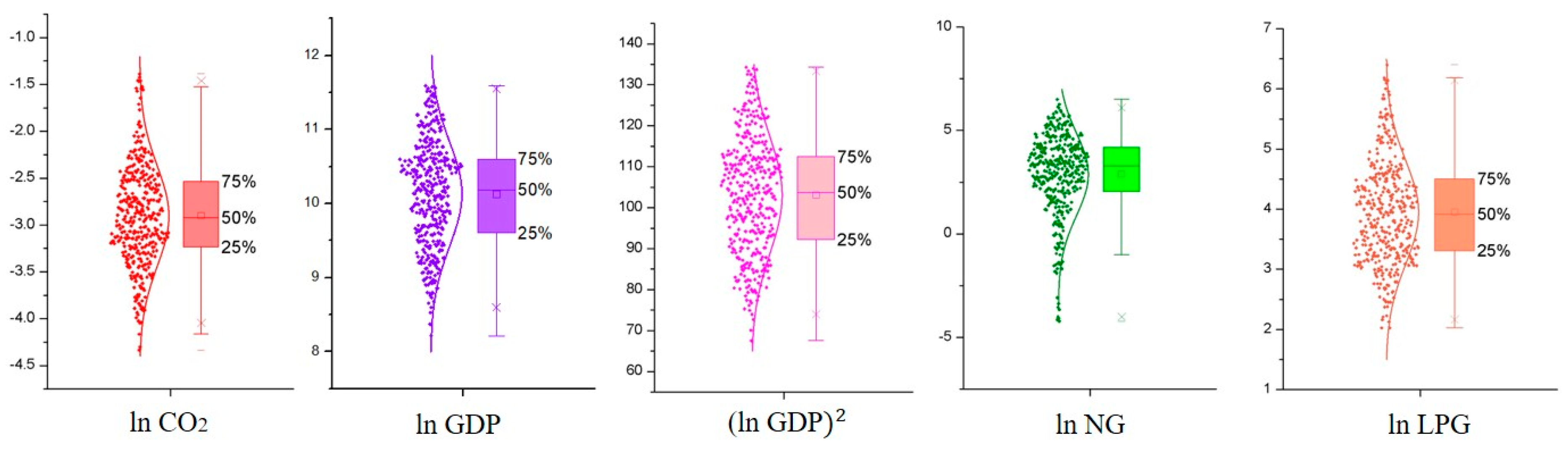
4.1. Results of Panel Unit Root Tests

The panel unit root test results are shown in

Table 3. Results of panel unit root tests.

Test	LLC		Fisher-PP
	Level	1st difference	Level	1st difference
$\ln C{O}_{2it}$	−4.557 ***	−7.004 ***	93.383 ***	218.159 ***
$\ln GD{P}_{it}$	6.835	−9.353 ***	23.886	141.950 ***
$(\ln GD{P}_{it}{)}^2$	6.869	−8.327 ***	26.017	126.602 ***
$\ln N{G}_{it}$	−32.665 ***	−18.989 ***	173.235 ***	281.838 ***
$\ln LP{G}_{it}$	−9.749 ***	−10.133 ***	131.685 ***	307.763 ***

Note: ***, **, and * indicate statistical significance at 1%, 5%, and 10%, respectively. Optimal lag lengths were selected automatically using the Schwarz information criteria. Legend: LLC, Levin-Lin-Chu; Fisher-PP, Fisher-Philips-Perron.

. As Table 3 shows, ln GDP and (ln GDP)² are not stationary at levels. The variables ln CO₂, ln NG, and ln LPG are stationary at levels. However, no unit root exists in the five time series that include ln CO₂, ln GDP, (ln GDP)², ln NG, and ln LPG at first-order difference, thus rejecting the null hypothesis [23,24]. The next step is to examine the relationship among CO₂ emissions, economic growth, natural gas, and liquefied petroleum gas.

4.2. Results of Cointegration Tests

As shown in

Table 4. Results of panel cointegration test. Legend: ADF, augmented Dickey-Fuller.

Pedroni residual cointegration test
Test	Intercept	Intercept and trend
Panel v-statistics	−2. 911	−4.970
Panel rho-statistics	2.999	4.392
Panel PP-statistics	−8.283 ***	−12.539 ***
Panel ADF-statistics	−5.531 ***	−7.666 ***
Group rho-statistics	6.202	7.167
Group PP-statistics	−16.879 ***	−30.619 ***
Group ADF-statistics	−7.263 ***	−10.413 ***
Kao residual cointegration test
Test	t-statistic
ADF	−5.076 ***

Notes: ***, **, and * indicate statistical significance at 1%, 5%, and 10%, respectively.

, the results indicate that four of the seven including the panel augmented Dickey-Fuller (ADF)-statistic, panel PP-statistic, group ADF-statistic, and group PP-statistic are significant at the 1% significance level. This indicates that the null hypothesis without cointegration is rejected. In addition, the Kao cointegration test also rejects the null hypothesis without cointegration. In summary, Pedroni and Kao cointegration tests show long-term relationships among CO₂ emissions, economic growth, natural gas and liquefied petroleum gas consumption. Also, this proves the existence of panel cointegration.

4.3. Estimation of Long-Run Coefficients

Since cointegration exists between the selected variables, as shown in

Table 5. Results of panel cointegration coefficient tests.

Test	Eastern	Central	Western	Northeast	China
FMOLS
$\ln GD{P}_{it}$	7.290 *** (0.944)	5.341 *** (1.032)	1.179 (0.956)	3.818 *** (0.907)	2.589 *** (0.560)
$(\ln GD{P}_{it}{)}^2$	−0.329 *** (0.043)	−0.248 *** (0.051)	−0.016 (0.052)	−0.161 *** (0.047)	−0.090 *** (0.028)
$\ln N{G}_{it}$	0.002 (0.018)	−0.013 (0.027)	−0.057 *** (0.016)	−0.009 (0.044)	−0.026 *** (0.010)
$\ln LP{G}_{it}$	0.068 * (0.042)	0.217 *** (0.071)	0.032 (0.048)	0.073 (0.067)	0.043 (0.027)
DOLS
$\ln GD{P}_{it}$	13.526 *** (1.580)	5.248 *** (0.891)	1.067 (1.025)	2.751 *** (0.902)	1.981 *** (0.603)
$(\ln GD{P}_{it}{)}^2$	−0.613 *** (0.072)	−0.244 *** (0.044)	−0.032 (0.051)	−0.115 ** (0.045)	−0.077 ** (0.030)
$\ln N{G}_{it}$	0.015 (0.038)	−0.001 (0.017)	−0.039 ** (0.019)	0.015 (0.050)	−0.020 * (0.011)
$\ln LP{G}_{it}$	0.243 *** (0.071)	0.160 ** (0.070)	0.019 (0.061)	0.093 (0.126)	0.019 (0.030)

Notes: ***, **, and * indicate statistical significance at 1%, 5%, and 10%, respectively. The values in brackets represent the std. error.

, this study estimates the long-term parameters for CO₂ emissions for each variable using FMOLS and DOLS estimation methods.

The long-term equilibrium of the whole sample indicates that the coefficients of ln GDP and (ln GDP)² are positively and negatively significant at the 1% level using the FMOLS and DOLS estimation methods. This indicates an inverted U-shape between China’s CO₂ emissions and economic growth. Thus, the EKC is assumed to be established. This is consistent with the findings of scholars such as Dong [22] and Kasman [41]. In addition, the coefficients of natural gas and liquefied petroleum gas consumption are negative and positive, respectively. According to FMOLS estimates, if natural gas consumption increases by 1%, CO₂ emissions are reduced by 0.026%, and 1% increase in liquefied petroleum gas consumption will grow CO₂ emissions by 0.043%. According to DOLS estimates, if natural gas consumption increases by 1%, CO₂ emissions are reduced by 0.020%, and 1% increase in liquefied petroleum gas consumption increases the emissions of CO₂ by 0.019%.

The long-term estimations at the four regional levels in China indicate that three of the four regions have more CO₂ emissions and are more affected by economic levels, supporting the existence of the EKC. However, CO₂ emissions in the western region are minor, and the economic level is relatively backward, so the EKC does not exist in western China. In addition, in eastern China, natural gas has a positive effect on CO₂ emissions, possibly because the economy level is high and the proportion of natural gas is relatively small compared to that of liquefied petroleum gas.

While natural gas consumption has a negative impact on CO₂ emissions in the central, western, and northeastern regions, the coefficient of natural gas consumption in the western region is particularly significant. This may be due to the abundant natural gas reserves in the western region and the proportion of natural gas consumption. Finally, liquefied petroleum gas consumption has a positive impact on CO₂ emissions in the eastern, central, northeastern, and western regions. In particular, the impact of liquefied petroleum gas consumption is significant in the eastern and central regions, indicating that liquefied petroleum gas consumption contributes to CO₂ emissions. The conclusion is that natural gas may have a negative effect on CO₂ emissions to a certain extent. Accelerating the development of natural gas energy can improve environmental quality and help to fight global warming.

4.4. The Results of the VECM Panel Granger Causality Test

As

Table 6. Panel vector error correction model (VECM) Granger causality analysis.

Dependent variable	Short run				Long run
	$\mathbf{\Delta }\mathbf{ln}\mathit{C}{\mathit{O}}_2{}_{\mathit{i}\mathit{t}-1}$	$\mathbf{\Delta }\mathbf{ln}\mathit{G}\mathit{D}{\mathit{P}}_{\mathit{i}\mathit{t}-1}$$(\mathbf{\Delta }\mathbf{ln}\mathit{G}\mathit{D}{\mathit{P}}_{\mathit{i}\mathit{t}-1}{}^2)$	$\mathbf{\Delta }\mathbf{ln}\mathit{N}{\mathit{G}}_{\mathit{i}\mathit{t}-1}$	$\mathbf{\Delta }\mathbf{ln}\mathit{L}\mathit{P}{\mathit{G}}_{\mathit{i}\mathit{t}-1}$	$\mathit{E}\mathit{C}{\mathit{T}}_{\mathit{i}\mathit{t}-1}$
	F-stat [p-value]				t-stat [p-value]
$\Delta \ln C{O}_2{}_{it}$	—	2.865 * [0.059]	2.094 [0.125]	0.239 [0.787]	2.247 ** [0.028]
$\Delta \ln GD{P}_{it}$ $(\Delta \ln GD{P}_{it}{}^2)$	1.839 [0.161]	—	1.486 [0.228]	0.967 [0.381]	5.066 *** [0.000]
$\Delta \ln N{G}_{it}$	9.187 *** [0.000]	2.299 [0.102]	—	0.937 [0.393]	−1.347 [0.179]
$\Delta \ln LP{G}_{it}$	1.215 [0.298]	0.335 [0.716]	0.062 [0.939]	—	0.910 ** [0.363]

Note: $\Delta$ indicates the first-difference operator; ***, **, and * are the 1%, 5%, and 10% levels of significance, respectively. The values in brackets represent the p-value.

shows, a causal relationship exists among CO₂ emissions, economic growth, and household fuel (natural gas and liquefied petroleum gas) consumption based on short-term and long-term panel VECM Granger causality tests. First, with regard to the long-term causality results, the t-statistics of CO₂ emissions, economic growth, and liquefied petroleum gas for ECT_t-1 are positive and significant. This indicates a long-term causal relationship among these three equations. This is consistent with the long-term estimates of FMOLS and DOLS. In the short term, one-way Granger causality runs from economic growth to CO₂ emissions and from CO₂ emissions to natural gas energy consumption. This means that a short-term causal effect exists between economic growth and CO₂ emissions and between CO₂ emissions and natural gas. These findings are consistent with Kasman [41], Hwang [42], and Zhang [43].

When examining the relationship between CO₂ emissions, economic growth, and household fuel (natural gas and liquefied petroleum gas) consumption, detecting the direction of causality is the most important step. The long-term effects of variables are particularly important and should make a huge contribution to the development of appropriate policies for the Chinese government to achieve CO₂ reduction.

5. Conclusions and Policy Implications

This study has used an unbalanced panel dataset for 30 provinces from 2003 to 2015 to validate the EKC hypothesis. By using unit root tests, panel cointegration tests, and VECM Granger causality tests, the novelty of this paper is that it is the first to study the long-term relationships among per capita CO₂ emissions, economic growth, and household fuel (natural gas and liquefied petroleum gas) consumption. Taking into account the differences in economic levels in various regions of China, the country was classified into four regions, namely, the eastern, central, western, and northeastern regions, and regression analysis was conducted on four sub-panels. Based on the results of FMOLS and DOLS estimation methods, the following conclusions can be drawn:

(1) Regarding the presence or absence of the EKC: At the national level, both FMOLS and DOLS estimation methods indicate an inverted U-shaped relationship between China’s CO₂ emissions and economic growth. The FMOLS and DOLS estimators demonstrate the presence of the EKC in the eastern, central, and northeastern regions; these three regions have more CO₂ emissions and are more affected by economic growth than the western region, which has less CO₂ emissions and a relatively backward economic level, so the EKC is not supported in western China. In short, the EKC is present at the national level and in the eastern, central, and northeastern regions. However, no EKC is seen in western China.

(2) Regarding the impact of household fuel (natural gas and liquefied petroleum gas) consumption on CO₂: At the national level, natural gas and liquefied petroleum gas consumption are negatively and positively correlated with CO₂ emissions. Among the four regions, natural gas consumption is positively correlated with CO₂ emissions in the eastern region, while it is negatively related to CO₂ emissions in the central, western, and northeastern regions, and the coefficient of natural gas consumption in the western region is particularly significant. Liquefied petroleum gas consumption has a positive impact on CO₂ emissions in the eastern, central, northeastern, and western regions. One important reason for high CO₂ emissions is the use of non-clean energy in China. At present, it is difficult to develop and apply high-efficiency energy technology in China, but the country is expected to implement fuel conversion as soon as possible to reduce CO₂ emissions. This is a good choice for developing countries like China.

The cost of natural gas and the pollution caused by purification processing is low. Natural gas can be used as a household gas or as an industrial chemical gas after simple purification processing and it emits less smoke after being fully burned. The main component of natural gas is 90–98% methane (CH₄), which only emits CO₂ and water after combustion. The composition of liquefied petroleum gas is relatively complicated, being mainly hydrocarbons of C₅-C₇. After liquefied petroleum gas combustion, the emissions of these components are various, and even some pollutants such as sulfur dioxide and hydrocarbons are emitted. Moreover, most liquefied petroleum gas is derived from petroleum, and more pollution is generated during the exploitation of oil. It is undeniable that the popularity of natural gas has a great impact on liquefied petroleum gas, but demand still exists in the liquefied petroleum gas market, which will be maintained for some time.

The change in energy structure has developed rapidly, and the proportion of natural gas in the energy structure has risen steadily and rapidly in China. The expansion of the natural gas pipeline means that the demand for natural gas consumption will continue to grow rapidly in the next few years. Although the output of natural gas is increasing, the rate of increase in output cannot keep up with the growth rate of consumption, and the gap between supply and demand is gradually widening. The exploitation of natural gas resources is limited in the short term and the construction of facilities is insufficient; the lack of supply in the natural gas market is also inevitable. To achieve the goal of sustainable development, every household needs to raise environmental awareness, save energy, and use clean fuel. China will also develop high-efficiency energy technologies rapidly, which will further promote CO₂ emissions reduction.

References

1. Grossman, G.M.; Krueger, A.B. Economic growth and the environment. Q. J. Econ. 1995, 110, 353–377. [Google Scholar] [CrossRef]
2. Green, F.; Stern, N. China’s changing economy: Implications for its carbon dioxide emissions. Clim. Policy 2017, 17, 423–442. [Google Scholar] [CrossRef]
3. Ouyang, X.; Lin, B. Carbon dioxide (CO2) emissions during urbanization: A comparative study between China and Japan. J. Clean. Prod. 2017, 143, 356–368. [Google Scholar] [CrossRef]
4. Shan, Y.; Liu, J.; Liu, Z.; Xu, X.; Shao, S.; Wang, P.; Guan, D. New provincial CO2 emission inventories in China based on apparent energy consumption data and updated emission factors. Appl. Energy 2016, 184, 742–750. [Google Scholar] [CrossRef]
5. Ouyang, X.; Lin, B. An analysis of the driving forces of energy-related carbon dioxide emissions in China’s industrial sector. Renew. Sustain. Energy Rev. 2015, 45, 838–849. [Google Scholar] [CrossRef]
6. Liu, Z.; Guan, D.; Wei, W.; Davis, S.J.; Ciais, P.; Bai, J.; Peng, S.; Zhang, Q.; Hubacek, K.; Marland, G.; et al. Reduced carbon emission estimates from fossil fuel combustion and cement production in China. Nature 2015, 524, 335. [Google Scholar] [CrossRef] [PubMed]
7. Grossman, G.M.; Krueger, A.B. Environmental Impacts of a North American Free Trade Agreement; National Bureau of Economic Research: Cambridge, MA, USA, 1991. [Google Scholar]
8. Shen, L.; Wu, Y.; Lou, Y.; Zeng, D.; Shuai, C.; Song, X. What drives the carbon emission in the Chinese cities?—A case of pilot low carbon city of Beijing. J. Clean. Prod. 2018, 174, 343–354. [Google Scholar]
9. Jalil, A.; Mahmud, S.F. Environment Kuznets curve for CO2 emissions: A cointegration analysis for China. Energy Policy 2009, 37, 5167–5172. [Google Scholar] [CrossRef]
10. Lindmark, M. An EKC-pattern in historical perspective: Carbon dioxide emissions, technology, fuel prices and growth in Sweden 1870–1997. Ecol. Econ. 2002, 42, 333–347. [Google Scholar] [CrossRef]
11. Heil, M.T.; Selden, T.M. Carbon emissions and economic development: Future trajectories based on historical experience. Environ. Dev. Econ. 2001, 6, 63–83. [Google Scholar] [CrossRef]
12. Moomaw, W.R.; Unruh, G.C. Are environmental Kuznets curves misleading us? The case of CO2 emissions. Environ. Dev. Econ. 1997, 2, 451–463. [Google Scholar] [CrossRef]
13. Selden, T.M.; Song, D. Environmental quality and development: Is there a Kuznets curve for air pollution emissions? J. Environ. Econ. Manag. 1994, 27, 147–162. [Google Scholar] [CrossRef]
14. Holtz-Eakin, D.; Selden, T.M. Stoking the fires? CO2 emissions and economic growth. J. Public Econ. 1995, 57, 85–101. [Google Scholar]
15. Sachs, J.; Panayotou, T.; Peterson, A. Developing Countries and the Control of Climate Change, Technical Report, CAER II, Discussion Paper. 1999.
16. Galeotti, M.; Lanza, A.; Pauli, F. Reassessing the environmental Kuznets curve for CO2 emissions: A robustness exercise. Ecol. Econ. 2006, 57, 152–163. [Google Scholar] [CrossRef]
17. Lantz, V.; Feng, Q. Assessing income, population, and technology impacts on CO2 emissions in Canada: Where’s the EKC? Ecol. Econ. 2006, 57, 229–238. [Google Scholar] [CrossRef]
18. Shafik, N.; Bandyopadhyay, S. Economic Growth and Environmental Quality: Time-Series and Cross-Country Evidence; World Bank Publications: Washington, DC, USA, 1992; Volume 904. [Google Scholar]
19. Friedl, B.; Getzner, M. Determinants of CO2 emissions in a small open economy. Ecol. Econ. 2003, 45, 133–148. [Google Scholar] [CrossRef]
20. Martínez-Zarzoso, I.; Bengochea-Morancho, A. Pooled mean group estimation of an environmental Kuznets curve for CO2. Econ. Lett. 2004, 82, 121–126. [Google Scholar] [CrossRef]
21. Dong, K.; Sun, R.; Hochman, G. Do natural gas and renewable energy consumption lead to less CO2 emission? Empirical evidence from a panel of BRICS countries. Energy 2017, 141, 1466–1478. [Google Scholar]
22. Dong, K.; Sun, R.; Hochman, G.; Zeng, X.; Li, H.; Jiang, H. Impact of natural gas consumption on CO2 emissions: Panel data evidence from China’s provinces. J. Clean. Prod. 2017, 162, 400–410. [Google Scholar] [CrossRef]
23. Dong, K.; Sun, R.; Li, H.; Liao, H. Does natural gas consumption mitigate CO2 emissions: Testing the environmental Kuznets curve hypothesis for 14 Asia-Pacific countries. Renew. Sustain. Energy Rev. 2018, 94, 419–429. [Google Scholar] [CrossRef]
24. Feng, T.; Sun, L.; Zhang, Y. The relationship between energy consumption structure, economic structure and energy intensity in China. Energy Policy 2009, 37, 5475–5483. [Google Scholar] [CrossRef]
25. Bhattacharya, M.; Paramati, S.R.; Ozturk, I.; Bhattacharya, S. The effect of renewable energy consumption on economic growth: Evidence from top 38 countries. Appl. Energy 2016, 162, 733–741. [Google Scholar] [CrossRef]
26. Alper, A.; Oguz, O. The role of renewable energy consumption in economic growth: Evidence from asymmetric causality. Renew. Sustain. Energy Rev. 2016, 60, 953–959. [Google Scholar] [CrossRef]
27. Dong, K.; Sun, R.; Dong, X. CO2 emissions, natural gas and renewables, economic growth: Assessing the evidence from China. Sci. Total Environ. 2018, 640, 293–302. [Google Scholar] [CrossRef] [PubMed]
28. Halicioglu, F. An econometric study of CO2 emissions, energy consumption, income and foreign trade in Turkey. Energy Policy 2009, 37, 1156–1164. [Google Scholar] [CrossRef]
29. Ozturk, I.; Acaravci, A. CO2 emissions, energy consumption and economic growth in Turkey. Renew. Sustain. Energy Rev. 2010, 14, 3220–3225. [Google Scholar] [CrossRef]
30. Acaravci, A.; Ozturk, I. On the relationship between energy consumption, CO2 emissions and economic growth in Europe. Energy 2010, 35, 5412–5420. [Google Scholar] [CrossRef]
31. Wang, S.S.; Zhou, D.Q.; Zhou, P.; Wang, Q.W. CO2 emissions, energy consumption and economic growth in China: A panel data analysis. Energy Policy 2011, 39, 4870–4875. [Google Scholar] [CrossRef]
32. Arouri, M.E.H.; Youssef, A.B.; M’henni, H.; Rault, C. Energy consumption, economic growth and CO2 emissions in Middle East and North African countries. Energy Policy 2012, 45, 342–349. [Google Scholar] [CrossRef]
33. Pao, H.-T.; Tsai, C.-M. CO2 emissions, energy consumption and economic growth in BRIC countries. Energy Policy 2010, 38, 7850–7860. [Google Scholar] [CrossRef]
34. Hossain, M.S. Panel estimation for CO2 emissions, energy consumption, economic growth, trade openness and urbanization of newly industrialized countries. Energy Policy 2011, 39, 6991–6999. [Google Scholar] [CrossRef]
35. Pao, H.-T.; Tsai, C.-M. Modeling and forecasting the CO2 emissions, energy consumption, and economic growth in Brazil. Energy 2011, 36, 2450–2458. [Google Scholar] [CrossRef]
36. Levin, A.; Lin, C.-F.; Chu, C.-S.J. Unit root tests in panel data: Asymptotic and finite-sample properties. J. Econ. 2002, 108, 1–24. [Google Scholar] [CrossRef]
37. Maddala, G.S.; Wu, S. A comparative study of unit root tests with panel data and a new simple test. Oxf. Bull. Econ. Stat. 1999, 61, 631–652. [Google Scholar] [CrossRef]
38. Pedroni, P. Panel cointegration: Asymptotic and finite sample properties of pooled time series tests with an application to the PPP hypothesis. Econ. Theory 2004, 20, 597–625. [Google Scholar] [CrossRef]
39. Kao, C. Spurious regression and residual-based tests for cointegration in panel data. J. Econ. 1999, 90, 1–44. [Google Scholar] [CrossRef]
40. Li, Y.; Sun, L.; Feng, T.; Zhu, C. How to reduce energy intensity in China: A regional comparison perspective. Energy Policy 2013, 61, 513–522. [Google Scholar] [CrossRef]
41. Kasman, A.; Duman, Y.S. CO2 emissions, economic growth, energy consumption, trade and urbanization in new EU member and candidate countries: A panel data analysis. Econ. Model. 2015, 44, 97–103. [Google Scholar] [CrossRef]
42. Hwang, J.-H.; Yoo, S.-H. Energy consumption, CO2 emissions, and economic growth: Evidence from Indonesia. Qual. Quant. 2014, 48, 63–73. [Google Scholar] [CrossRef]
43. Zhang, X.-P.; Cheng, X.-M. Energy consumption, carbon emissions, and economic growth in China. Ecol. Econ. 2009, 68, 2706–2712. [Google Scholar] [CrossRef]
Figure 1. Distribution of CO2 emissions and household fuel (natural gas and liquefied petroleum gas) consumption in China in 2015. Note: Tibet, Hong Kong, Macao, and Taiwan were not considered due to data unavailability.
Sustainability 11 00979 g001
Figure 2. Scatter plot and distribution of all variables after logarithm. Note: The dots denote the minimum/maximum values and the triangles refer to the mean values.
Sustainability 11 00979 g002