Spatiotemporal Features and Socioeconomic Drivers of PM_2.5 Concentrations in China

Abstract

Fine particulate matter (PM_2.5) has been an important environmental issue because it can seriously harm human health and can adversely affect the economy. It poses a problem worldwide and especially in China. Based on data of PM_2.5 concentration and night light data, both collected from satellite remote sensing during 1998–2013 in China, we identify the socio-economic determinants of PM_2.5 pollution by taking into account the spatial flow and diffusion of regional pollutants. Our results show PM_2.5 pollution displays the remarkable feature of spatial agglomeration. High concentrations of PM_2.5 are mainly found in Eastern China (including Shandong, Jiangsu, and Anhui provinces) and the Jing-Jin-Ji Area region in the north of China (including Beijing, Tianjin, and Hebei provinces) as well as in the Henan provinces in central China. There is a significant positive spatial spillover effect of PM_2.5 pollution, so that an increase in PM_2.5 concentration in one region contributes to an increase in neighboring regions. Whether using per capita GDP or nighttime lighting indicators, there is a significant N-shaped curve that relates PM_2.5 concentration and economic growth. Population density, industrial structure, and energy consumption have distinct impacts on PM_2.5 pollution, while urbanization is negative correlated with PM_2.5 emissions. As a result, policies to strengthen regional joint prevention and control, implement cleaner manufacturing techniques, and reduce dependence on fossil fuels should be considered by policy makers for mitigating PM_2.5 pollution.

1. Introduction

As the acceleration of industrialization and urbanization in recent years, air quality continues to deteriorate in China, resulting in increased threats to human health and sustainable economic development. Since 2013, several large-scale and long-duration haze incidents have taken place in China, and the whole society is now more concerned about air pollution problems, especially PM_2.5 (fine particulate matter that is 2.5 micrometers or less in diameter). PM_2.5 is rich in many toxic organic components and easily reaches the lungs when inhaled. Exposure to high PM_2.5 levels for a long time constitutes a significant health risk. Previous research has found that PM_2.5 pollution is strongly associated with many diseases, including asthma, lung cancer, and heart disease [1,2,3,4]. Research indicates that the number of premature deaths owing to outdoor air pollution is estimated to be between 350,000 and 500,000 annually in China [5]. Premature deaths, loss of working hours, and related welfare expenses caused by air pollution have resulted in an estimated GDP loss of 10% in China [6]. In addition, PM_2.5 pollution poses a great threat to economic growth, traffic safety, climate change, and so on [7,8,9,10,11].

In response to the frequent occurrence of fog and haze pollution, the administrative department has formulated a series of policies to mitigate atmospheric pollution in China [12]. For instance, the Chinese Ministry of Environmental Protection released a new Ambient Air Quality Standard in 2012, which includes a PM_2.5 concentration monitoring index for the first time and takes PM_2.5 concentration as the main control objective for improving air quality. According to the new standard, the upper limit of the average concentration of PM_2.5 is 35 μg/m³ in China [13]. Besides, an Action Plan for Air Pollution Prevention and Control was issued in 2013, which promises that concentration of hazardous particles including PM_2.5 will be reduced by about 10% below the 2012 level.

PM_2.5 pollution correlates not only with chemical and physical factors such as temperature, wind speed, and climate, but also with social and economic factors. Many previous studies focused on the main chemical mechanism of haze formation in China [14,15,16]. However, few studies have quantitatively measured socioeconomic factors that affect PM_2.5 emissions, which remain poorly understood in China [17,18]. Therefore, if we are to mitigate pollution, it is crucial to identify the key anthropogenic effect factors on PM_2.5 emission. The objective of this research was to explore the causes of PM_2.5 pollution from the perspective of economic and social factors. Specifically, we applied a spatial econometric model to explore the influence of economic growth, population density, urbanization, industrialization, and energy consumption on PM_2.5 concentrations. In addition, we investigated the spatiotemporal patterns and spatial correlations of PM_2.5 pollution to provide a scientific reference for policy makers.

2. Literature Review

As is well known, the relationship between economic growth and environmental pollution has always been one of the central issues in environmental economics. Many studies have focused on this topic, and there have been some empirical tests based on the Environmental Kuznets Curve (EKC) hypothesis put forward by Grossman and Krueger [19]. The EKC hypothesis states that there is an upside-down U-shaped relationship between pollution emission and growth—that is, at the beginning of economic developing, environmental pollution increases as income rises, but beyond a certain inflection point, pollution declines with increased income [20]. Although some research results support the inverted U hypothesis [21,22,23], other studies provide inconsistent or even opposite evidence [24,25,26]. Overall, the results suggest that there may exist complicated relationship between economic growth and environmental quality.

Most of the studies on the EKC hypothesis examined the relationship between per capita GDP and different pollutants, including mainly CO₂, SO₂, NOx, CO, water pollution, and solid waste. Many studies confirm the existence of a typical upside-down U curve between environmental pollution and economic growth. For instance, Fosten et al. [23] investigated the EKC hypothesis by using UK data and found that an upside-down U curve exists between CO₂ and SO₂ emissions and income. The empirical results of Apergis and Ozturk [27] confirm the existence of converse-U correlativity between economic developing and CO₂ emissions for fourteen Asian countries. Lin and Liscow [28] provided evidence supporting an inverted-U shaped curve for seven out of 11 water pollutants in China. However, some studies got different results and challenged the inverted-U hypothesis. In these studies, researchers found a variety of relationships between economic growth and pollution emission, such as a linear relationship [29,30], a U-shaped relationship [31], an N-shaped relationship [32], or even an inverted N-shaped relationship [33]. Moreover, a few researchers find no evidence of a significant relationship between pollution emissions and economic growth. Since the conclusions depend mainly on the selection of pollutants and the choice of econometric technique, the findings provide mixed conclusions about the EKC hypothesis [34].

To better explain the environmental impacts, subsequent empirical study on the relationship between air pollution and economic development often incorporated other socioeconomic factors than per capita income that may affect air quality. These factors, including but not limited to urbanization, energy consumption, population density, and industrial structure, have also been introduced into EKC studies. Energy consumption is often taken as an important determinant of pollution emissions. Many empirical studies confirm that higher energy consumption produces more pollution emissions [35,36]. Moreover, some researchers stress that rapid industrialization requires a great deal of energy consumption and, correspondingly, more pollution emissions [37,38]. For example, Li et al. [39] have confirmed that the expansion of secondary industries has notable positive influence on seven pollutant emissions. Moreover, population density and urbanization are also often seen as factors affecting air quality [38,40]. By using the Geographical Weighted Regression (GWR) model, Fang [41] found that population and urbanization have remarkable influence on air quality. Ma et al. [42] also found that higher population density and rate of urbanization lead to more resource consumption and more pollution emissions, which affect environmental quality. However, the results of Luo et al. [37] show that although urbanization is a decisive factor in pollution emission, the impact varies across regions, while population density plays a weak role. Thus, the empirical results indicate that urbanization and population density have ambiguous effects on air quality and need further research [37].

Although there is a growing literature dealing with the EKC hypothesis for different pollutants, such as CO₂, SO₂, and NOx, researchers have paid little attention to the relationship between economic growth and PM_2.5 emission [37,43]. For a developing country such as China, the lack of stable and reliable long-term detection data is a major obstacle for PM_2.5 pollution research. Only in recent years has PM_2.5 concentration been monitored in China. With advances in technology, the total-column aerosol optical depth (AOD) observed by satellites can provide spatially continuous information of PM_2.5 concentrations. Moreover, existing reports seldom consider the spatial correlation and spatial spillover effects when analyzing the factors affecting air pollution [44,45]. In fact, haze pollution has significant spatial diffusion [42]. Air pollution is not a simple local environmental issue but to a large extent a broader regional problem because it will spread or transfer to adjacent regions through natural factors such as atmospheric circulation, atmospheric chemical action, and economic mechanisms such as pollution leakage, industrial transfer, industrial agglomeration, and traffic flow. Therefore, the results found using some traditional econometric methods such as ordinary least square (OLS) and generalized least squares (GLS) may be invalid or biased when applied to factors affecting haze pollution. In order to effectively avoid estimation bias caused by ignoring spatial correlation, this research chooses the proper spatial panel model to study the influencing factors in the spatial spillover effect of PM_2.5 pollution.

It is also important to emphasize that China’s GDP statistical systems and accounting methods are relatively backward [46], with some suspicion about whether official statistics are entirely reliable [47]. Recent studies have begun to use the nighttime satellite lighting data published by the US National Oceanic and Atmospheric Administration (NOAA) to measure economic growth [48,49,50]. Different from the traditional use of GDP to measure the level of economic development, satellite lighting data is not affected by regional price factors. Besides, it includes not only market economy goods and services measured by GDP but also non-market factors [51]. Recognizing that there is some question about the authenticity of China’s statistics, this paper carries out a more robust empirical test of PM_2.5 pollution and the EKC hypothesis by using satellite lighting data as an alternative to GDP.

This study fills gaps in previous studies in the following ways. First, taking into account the spatial dependence effect of PM_2.5 emission, we use the spatial panel model to investigate factors that influence PM_2.5 pollution. We selected the most appropriate spatial econometric model from the three kinds of common spatial regression models. We then effectively avoid estimation error caused by ignoring spatial autocorrelation of space units. Second, in view of the doubts about the authenticity of China’s economic statistics, this paper uses nighttime lighting data of satellite monitoring as a proxy variable for economic growth, allowing for a more robust empirical test of the EKC hypothesis of PM_2.5 pollution.

The balance of this article is arranged as below: Data collection and model methods are introduced in Section 3. Results of socio-economic factors affecting haze concentration are presented in Section 4. In a final Section 5, we summarize our research findings and make some policy recommendations.

3. Research Methods and Data

3.1. Exploratory Spatial Data Analysis

Before using a spatial econometric technique, one must establish a spatial dependence. In this study, we apply Global Moran’s I index to analyze the overall spatial autocorrelation of provincial PM_2.5 emission. The Global Moran’s I can be presented as

$$\mathrm{I}=\frac{{\sum }_{i=1}^n{\sum }_{j=1}^n{w}_{ij}{A}_i-\overline{A}{A}_j-\overline{A}}{S^2{\sum }_{i=1}^n{\sum }_{j=1}^n{w}_{ij}}$$

(1)

$$S^2=\frac{1}{n}{\displaystyle \sum }_{i=1}^n{A}_i-{\overline{A}}^2, \overline{A}={\displaystyle \sum }_{i=1}^n{A}_{i }, -1\le I\le 1$$

(2)

I indicates the overall correlation degree of inter-regional PM_2.5 concentration. The closer the I value is to 1, the stronger the positive autocorrelation between regions, and the closer tended toward –1, the higher the negative autocorrelation, A value of 0 means that there is no spatial autocorrelation. A_i is the PM_2.5 concentration value of the i area, n represents the area number, and W indicates the spatial weight matrix. We set the weight matrix as follows:

$$\mathrm{w}=\left[\begin{array}{ccc}{w}_{11}& w_{12}& \begin{array}{cc}\dots & w_{1n}\end{array}\\ w_{21}& w_{22}& \begin{array}{cc}\dots & w_{2n}\end{array}\\ \begin{array}{c}⋮\\ w_{n1}\end{array}& \begin{array}{c}⋮\\ w_{n2}\end{array}& \begin{array}{cc}\begin{array}{c}⋮\\ \dots \end{array}& \begin{array}{c}⋮\\ w_{nn}\end{array}\end{array}\end{array}\right]$$

(3)

Here n represents the total number of areas to be studied, W_ij indicates the adjacent relationship between region i and region j. If they have common vertices or common edges, w_ij = 1, otherwise w_ij = 0.

Global Moran’s I characterize the spatial clusters of PM_2.5 concentrations as a whole. However, the index ignores the potential instability of the spatial process and does not reflect the spatial heterogeneity of the internal units of the region [52]. The Local Indicators of Spatial Association (LISA) can test whether the spatial clusters are significant or not. This article uses the Local Moran’s I to measure the local autocorrelation, and then conducting significance test of Moran’s I. The formula is as below.

$$I_t=\frac{\left(A_i-\overline{A}\right)}{S^2}{{\displaystyle \sum }}_{i=1}^n{W}_{ij}{A}_j-\overline{A}$$

(4)

Here, S² and$\overline{A}$ are the same as in Equation (1); I_i is the local Moran’s I of region i, which measures the PM_2.5 association of the i area and its neighboring area. I_i > 0 indicates positive correlation. I_i < 0 shows negative correlation.

3.2. Spatial Panel Data Model

3.2.1. Model Specification

The EKC hypothesis argues that environmental pollution and per capita income existing inverted-U relationship. Supplementing the EKC model, this paper introduces urbanization, energy consumption, industrial structure, and population density into the model. The extended EKC model is as follows:

$$Lnp{m}_{it}={\alpha }_{it}+{\beta }_{1}Ln\left(y_{it}\right)+{\beta }_2{\left(Ln{y}_{it}\right)}^2+{\beta }_3{\left(Ln{y}_{it}\right)}^3+{\beta }_{4}u{r}_{it}+{\beta }_{5}Ln\left(e{n}_{it}\right)+{\beta }_{6}in{s}_{it}+{\beta }_{7}Ln\left(p{d}_{it}\right)+{\epsilon }_{it}$$

(5)

Here, Ln is logarithmic forms of variable, pm_it denotes PM_2.5 concentration, y represents economic growth, ur is the urbanization rate, en stands for energy consumption, ins is industrial structure, pd is the population density, and ε means the standard error term.

3.2.2. Spatial Econometric Method

Because of the heterogeneity and autocorrelation of spatial units, the results estimated are biased and invalid by the traditional econometric method based on hypothesis of homoscedasticity and cross-section independence. Spatial econometrics model can effectively deal with spatial interaction between geographic units. In fact, PM_2.5 emission generated in one region generally diffuses to surrounding regions due to of wind and other factors. That is, the observations are not independent of each other and have a strong spatial dependence. Therefore, since the traditional OLS regression method will cause biased estimation result due to spatial correlation, this study uses a spatial econometric model to measure spatial spillover effects. There are three kinds of common spatial econometric models: SLM, SEM, and SDM.

The Spatial Lag Model (SLM) focuses on testing whether a variable experience a diffusion effect in a certain area—i.e., whether there is a spatial spillover effect. It takes into account that an observed value of a dependent variable in a certain region may depend in part on a spatially weighted average of the values of that dependent variable in adjacent regions. The SLM model can be presented as follows:

$$y_{it}=\delta {\displaystyle \sum }_{j=1}^n{w}_{ij}{y}_{jt}+\beta x_{it}+{\mu }_i+{\lambda }_t+{\epsilon }_{it}$$

(6)

Here, y_it indicates the i-th region’s PM2.5 concentration at time t. δ is the spatial autocorrelation coefficient, w_ij is the spatial weight matrix N×N. β represents the unknown parameter vector of the independent variable x_it. The term μ_i represents a regional fixed effect and λ_t denotes a time-period specific effect. ε_it indicates a random error term, which obeys a standard normal distribution (0,σ²).

The Spatial Error Model (SEM) is a method for dealing with spatial dependence of error terms. It can be seen as a combination of standard regression models and spatial autoregressive models of error terms. The SEM is specified as follows:

$$y_{it}=\beta x_{it}+{\mu }_i+{\lambda }_t+{\phi }_{it}, {\phi }_{it}=\rho {\displaystyle \sum }_{j=1}^n{w}_{ij}{\phi }_{it}+{\epsilon }_{it}$$

(7)

Here, the φ_it term represents the spatially autocorrelated error term and ρ denotes the spatial autoregressive coefficient of the error term.

In order to overcome some defects of the SLM and SEM models, Le Sage and Pace [53] proposed the spatial Dubin model (SDM), which contains the lagged terms of the interpreted variables and the explanatory variables. The spatial Durbin model is expressed as follows:

$$y_{it}=\delta {\displaystyle \sum }_{j=1}^n{w}_{ij}{y}_{jt}+\beta x_{it}+{\displaystyle \sum }_{j=1}^n{w}_{ij}{x}_{it}\gamma +{\mu }_i+{\lambda }_t+{\epsilon }_{it}$$

(8)

Here, γ is a vector (k×1) of the spatial autocorrelation coefficient of the explanatory variable. Equation (8), if appropriately constrained, can describe all three models. If γ = 0, the model is simplified to SLM. If γ+ δβ = 0, the model is simplified to SEM.

Since the estimation model includes the spatially lagged explanatory variables and interpreted variables, it is hard to accurately measure the effects of the independent variable on the dependent variable. LeSage and Pace [53] pointed out that using point estimation method may lead to erroneous conclusions when used to test whether there is spatial spillover effect in a spatial regression model. According to their suggestions, it is valid to use a partial derivative to measure the impact of changing the explaining variable on the explained variable. The effects of independent variables on the dependent variables can be divided into three effects: The first is the direct effect; that is, the explained variable is affected by the changing of explanatory variable in the region. The second is the indirect effect; that is, the impact of changing the factor in the region on dependent variable in all other region. The third is the total effect; that is, the sum of these impacts.

In this paper, the general least squares (OLS) method is employed to estimate the non-spatial panel data model. However, if the estimation of the spatial model uses OLS method, the coefficient estimates will be biased or invalid [54]. So, the maximum likelihood (ML) method is employed to estimate spatial model parameter. The model fitting effect is tested by the R² and Log- likelihood function values.

3.3. Data Collection

The PM_2.5 data which are estimated by combining Aerosol Optical Depth retrievals are collected from the Atmospheric Composition Analysis Group/Dalhousie University. The validation of satellite-derived estimates has been confirmed by empirical research, which suggests they are generally consistent with ground-based PM_2.5 measurements [55]. We used ArcGIS to extract a dataset and obtained data on PM_2.5 concentrations for 31 provinces in China during the sample period.

The night light data used in this study came from the global DMSP/OLS nighttime light remote sensing data posted on the National Oceanic and Atmospheric Administration (NOAA) website. The data about China’s local administrative regions come from the 1:4 million vector maps provided by the China National Basic Geographic Information Center. This article uses ArcGIS software to extract data of China provincial administrative regions from the global nighttime lighting data during 1998-2013. To improve the accuracy of the data, we drew on Liu’s suggestion [56] and processed the lighting data by inter-calibration and intra-annual composition methods to reduce the measurement error of the data. In this paper, the intensity of each grid is summed up as a measure of its total light data in the provincial area. The night light data divided by the number of permanent residents of each province (in units of 10,000) are used as a substitute for per capita GDP in each year.

The urban population ratio of total population is selected to measure urbanization rate. Industrial structure is measured by the fraction of secondary industry among gross domestic product. The number of people per square kilometer is used to measure population density. Energy consumption is measured by per capita energy consumption. Economic growth is expressed by GDP (1998 constant price) divided by the total population at year-end. The research period covers the years 1998-2013 for 31 provinces of China, not including Taiwan province, Macao, and Hong Kong special administration regions due to missing data. All of these data are extracted from the Chinese statistical yearbook between 1998 and 2013 and China Energy Statistical Yearbook from 1998 to 2013.

4. Results

4.1. Spatiotemporal Patterns of PM_2.5 Concentration

4.1.1. Spatial Distribution of PM_2.5 Concentration

Based on the air quality guidelines published by the World Health Organization (WHO) in 2005, this paper divides the China’s PM_2.5 densities in μg/m³ into five levels: Level I (<10), Level II (10–15), Level III (15–35), Level IV (35 –50), and Level V (>50). There are obvious regional differences in the distribution of China’s PM_2.5 pollution. As shown in Figure 1, Levels I and II are mainly scattered in areas such as Qinghai-Tibet Plateau and the northwest including the Xinjiang, Gansu, and Inner Mongolia provinces, which are west of Hu’s line. PM_2.5 concentration in most of these areas is lower than 10 μg/m³, which is the WHO standard for acceptable air quality. Level III, Level IV, and Level V are mainly located east of Hu’s line, which forms a west-east divide between low and high PM_2.5 concentration. It is noteworthy that the regions of Level IV and Level V continued to sprawl during the sample period, reflecting the trend toward rising PM_2.5 emission in China. Level V—that is, the highest concentration level—is mainly found scattered in the Beijing-Tianjin-Hebei region in northern China; Henan province of Central China; and Shandong, Jiangsu, and Anhui provinces of Eastern China. These provinces not only have a high density of economic activities and coal-based industries but are also adjacent to each other. Therefore, the degree of environmental pollution shows obvious spatial dependence.

4.1.2. Features of PM_2.5 Concentration Variation

As illustrated in Figure 2, the annual average value of China’s PM_2.5 pollution shows a fluctuating pattern from 1998 to 2013. The average PM_2.5 concentration value was 26.07 μg/m³ in 1998, following which it increases to 40.32 μg/m³ in 2007, then slowly dropped to 33.83 μg/m³ in 2012, and later rose again to 39.78 μg/m³ in 2013. It is noteworthy that the variation coefficient of PM_2.5 concentration was between 0.3 and 0.5 in 1998-2013, and the overall fluctuation range has been relatively stable. The variation coefficient showed a noticeable increase from 1998 to 2006 and then decreased slowly from 2007 to 2013. This implies that the regional differences of China’s PM_2.5 concentration had a trend of expansion from 1998 to 2006 and shrunk progressively between 2007 and 2013.

In order to intuitively describe the dynamic evolution and distribution features of PM_2.5 concentration, this study used the kernel density distribution to analyze its dynamic changes. Figure 3 depicts the kernel density evolution path of PM_2.5 emissions in 31 provinces of China between 1998 and 2013. In general, the shape of the distribution curve of PM_2.5 emissions changed significantly over the studied period and the curve itself moved to the right, implying that PM_2.5 concentrations increased during the studied period. From the changes in the kurtosis of the density distribution curve, it is easy to see that the pattern of the haze pollution changed considerably from a sharp peak at lower concentrations to a broad peak at higher concentrations, meaning the increase of regional PM_2.5 concentration difference in China.

4.2. Spatial Autocorrelation Test

Table 1. Global Moran’s I index of China’s PM_2.5 concentration during 1998–2013.

	I	Z	P
1998	0.295	3.028	0.001
1999	0.237	2.476	0.007
2000	0.361	3.618	0.000
2001	0.350	3.554	0.000
2002	0.392	3.905	0.000
2003	0.470	4.653	0.000
2004	0.408	4.071	0.000
2005	0.473	4.669	0.000
2006	0.444	4.439	0.000
2007	0.499	4.897	0.000
2008	0.457	4.533	0.000
2009	0.430	4.310	0.000
2010	0.440	4.367	0.000
2011	0.473	4.686	0.000
2012	0.450	4.453	0.000
2013	0.435	4.371	0.000

demonstrates the Global Moran’s I index of China’s PM_2.5 concentration during 1998-2013. Results of Moran’s I are all significantly positive, which suggests that there is a positive spatial autocorrelation in PM_2.5 concentration. In addition, Global Moran’s I index value also showed a rising trend although it fluctuated slightly during the study period, increasing from 0.295 in 1998 to 0.435 in 2013, implying that the degree of spatial agglomeration of PM_2.5 pollution is gradually increasing in China over time.

Figure 4 illustrates the scatter plot of the distribution of provincial PM_2.5 concentration under the geospatial weight matrix for 1998, 2003, 2008, and 2013. The vertical axis signifies the spatial lag value of the PM_2.5 concentration; the horizontal axis shows the normalized PM_2.5 concentration. These axes divide the PM_2.5 pollution clusters into four types of spatial correlation (high-high, low-high, low-low, and high-low). From Figure 4, we can see that most of the provinces are situated in the upper right quadrant and the lower left quadrant, which further illustrates the significant high-pollution and low-pollution clustering characteristics for PM_2.5 pollution in China.

Local spatial clusters maps are shown in Figure 5, based on local Moran’s I index. Five regions are distinguished: a High-High (HH) area denoted by red color, a High-Low (HL) area denoted by green color, a Low-Low (LL) area denoted by blue color, a Low-High (LH) area denoted by orange color, and areas are not related in a spatially significant manner by gray color. From 1998 to 2013, there was a slight increase in provinces located in High-High areas. In 1998, only Beijing, Henan, and Shandong provinces were situated in a HH area. However, in 2003, 2008, and 2013, there were, respectively, 6, 5, and 5 provinces located in High-High areas. These H-H provinces are mainly scattered in Beijing-Tianjin-Hebei and East China, and include Beijing, Hebei, Tianjin, Shandong, Anhui, and Jiangsu provinces. The Low-Low areas are concentrated in the southwest of China, and include Yunnan, Sichuan, Tibet, Qinghai, and Guizhou provinces in four representative years. Xinjiang and Hainan are of the L-H and H-L cluster type, respectively. These results are basically consistent with the above conclusions about the spatial distribution of PM_2.5 concentration. The H-H area is a region with a high level of economic development and high concentration of industrial economic activity. The autocorrelation between these regions in economic space relates to a high dependence on air pollution, making these regions high concentration areas for PM_2.5.

4.3. Empirical Results

4.3.1. Estimated Result

For the specification of the model, we first made estimates based on non-spatial panel data models, and then distinguished whether the spatial dependence of sample data is present or not by employing the Lagrange Multiplier (LM) test and Robust Lagrange Multiplier (RLM) test. As

Table 2. Diagnostic tests of model specification (per capita GDP).

Determinants		Determinants
LM spatial lag	16.508 ***(0.000)	Wald test spatial lag	41.22 ***(0.000)
Robust LM spatial lag	69.946 ***(0.000)	LR test spatial lag	37.46 ***(0.000)
LM spatial error	80.516 ***(0.000)	Wald test spatial error	22.90 ***(0.001)
Robust LM spatial error	69.946 ***(0.000)	LR test spatial error	22.72 ***(0.001)

Note: ***, **, or * represent 1%, 5%, or 10% thresholds of significance, respectively.

shows, the results of the LM test and the RLM test are significant at the 1% level, implying that the original hypothesis of no spatially auto-correlated error term can be refused. As a result, spatial panel models are suitable for the estimation of sample data.

To determine which spatial econometric model is most suitable for dealing with spatial dependence, this study used the SDM model estimation and then performed the Wald test and likelihood ratio (LR) test. The outcomes of testing significantly reject the null hypothesis that there is no spatial lag and no spatial error at the 1% level (Table 2). Moreover, the R² and log-likelihood value of the SDM model are higher than for other models. As a result, the SDM model, which includes features of both SEM and SLM, is most suitable for our sample analysis. In addition, the Hausman test results 36.73, p < 0.001, show that the SDM model with fixed effect model is most suitable for model specifications.

Table 3. Parameter summary of estimation results (per capita GDP).

	Pool ols		SLM		SEM		SDM
	Coef.	t	Coef.	z	Coef.	z	Coef.	z
intercept	−77.90 ***	25.780
ur	−0.311	0.223	−0.323	0.242	−0.354	0.225	−0.490 **	0.243
ins	1.068 ***	0.260	1.106 ***	0.236	0.942 ***	0.200	0.871 ***	0.241
lnpd	0.207 ***	0.013	0.151 ***	0.012	0.205 ***	0.015	0.203 ***	0.018
lnen	0.389 ***	0.045	0.375 ***	0.042	0.311 ***	0.041	0.338 ***	0.044
lny	24.850 ***	8.203	24.72 ***	7.160	23.57 ***	6.960	20.400 ***	7.070
(lny)2	−2.655 ***	0.868	−2.667 ***	0.757	−2.487 ***	0.738	−2.136 ***	0.750
(lny)3	0.0938 ***	0.030	0.095 ***	0.027	0.087 ***	0.026	0.074 ***	0.026
W *ur							−0.072	0.464
W *ins							−0.888	0.543
W *lnpd							-0.105 ***	0.031
W *lnen							0.056	0.079
W *lny							−24.330 *	13.56
W *lny2							2.435 *	1.443
W *lny3							−0.081	0.051
ρ			0.484 ***	0.045			0.623 ***	0.051
λ					0.650 ***	0.048
σ2			0.088 ***	0.005	0.080 ***	0.005	0.078 ***	0.005
R2	0.580		0.586		0612		0.622
Log-likelihood			−114.808		−109.572		−98.214

Note: ***, **, or * represent 1%, 5%, or 10% thresholds of significance, respectively.

reports the empirical results of the Pooled OLS model, SLM model, SEM model, and SDM model.

The spatial correlation coefficient ρ in the SDM model is significantly positive, suggesting that there is a strong spatial spillover effect in PM_2.5 pollution in China. The finding shows PM_2.5 pollution is affected by the economic and social factors in the region and by pollution in neighboring areas; that is, the rise of PM_2.5 emission in neighboring provinces will increase the level of provincial pollution. The spatial spillover effect further proves the appropriateness of using spatial econometric analysis tools and also provides a theoretical basis for the strategies of inter-regional prevention and control of pollution.

The coefficients of industrial structure, population density, and energy consumption are significantly positive, suggesting that a higher share of secondary industry in the GDP and more population agglomeration increase PM_2.5 pollution. Contrary to expectations, the coefficient of urbanization rate is significantly negative, which means that the PM_2.5 emissions decline with growing urbanization. This result seems surprising and is different from most existing research conclusions. However, as the urbanization rate increases, the public’s requirements for environmental quality are correspondingly increased. Under the pressure of public opinion, the government introduced stricter environmental regulation policies, which led to the transformation of industrial structure from high-pollution industries to low-emission tertiary industries. This result can significantly reduce pollution emissions. Moreover, some researchers have found that rural energy consumption is an important source of PM_2.5 pollution. Urbanization can also significantly reduce this part of pollution emissions [57].

It is a focus of special interest that for the coefficients of income, the quadratic term and the cubic term for three models are significantly positive, negative, and negative, respectively. According to the estimated results, we can conclude that there exists an N-shaped curve between economic growth and PM_2.5 pollution, implying that PM_2.5 emissions first increased, then decreased, and then increased again with GDP per capita growth during the observed period.

The product terms of the spatial weight’s matrix W and independent variables in the model mirror how these variables in neighboring provinces affect the provinces’ PM_2.5 pollution. The coefficients of W*ur, W*ins, W*lnpd, and W*lny are negative, meaning that increases of urbanization rate, secondary industry, population density, and per capita GDP in nearby provinces will mitigate provincial PM_2.5 pollution, although only two parameters passed the significance test. One possible explanation is that the demand for environmental quality increases as incomes rises in neighboring areas, which may diminish spillover effects on provincial pollution emissions. In addition, the fact that the coefficients of W*lnen are insignificant indicates that the spatial effects of energy consumption on PM_2.5 pollution is trivial.

4.3.2. Direct and Indirect Effects of SDM Estimates

In order to explore the interaction information contained in the regression coefficients, we give the estimated results of the direct effect, indirect effect, and total effect of variables. As displayed in

Table 4. The effects measurement of Spatial Dubin Model (per capita GDP).

	Direct	z	Indirect	z	Total	z
ur	−0.586 **	0.287	−0.989	1.232	−1.575	1.422
ins	0.785 **	0.317	−0.898	1.424	−0.113	1.679
lnpd	0.209 ***	0.0161	0.0531	0.054	0.262 ***	0.056
lnen	0.396 ***	0.0512	0.660 ***	0.214	1.056 ***	0.246
lny	18.06 **	8.075	−28.42	32.41	−10.36	37.05
(lny)2	−1.916 **	0.854	2.700	3.437	0.785	3.923
(lny)3	0.067 **	0.030	−0.084	0.121	−0.017	0.138
turning points	5039/37786

Note: ***, **, or * represent 1%, 5%, or 10% thresholds of significance, respectively.

, the coefficient of the direct effect is similar to the estimated coefficient of the Spatial Dubin Model in Table 3, with subtle changes due to spatial feedback effects. The direct effects of urbanization rate, industrial structure, population density energy consumption, and GDP per capita are –0.586, 0.785, 0.209, 0.396, and 18.06, respectively. Among them, the direct effect of per capita GDP is larger than others, meaning economic growth is a major factor affecting the PM_2.5 emission in the province. A positive change of income by 1% will increase the PM_2.5 concentration of the province by approximately 18%. For indirect effects, only the parameter of energy consumption passed the significance test, which shows that energy consumption will not only increase pollution in the province but also increase pollution in neighboring provinces. A positive change of energy consumption by 1% will increase PM_2.5 concentration by approximately 0.7% in neighboring provinces.

According to the results shown in Table 4, the direct effect for income (the linear term), the quadratic term, and the cubic term are significantly positive, negative, and positive, respectively. Therefore, the discussions for estimated results are similar to those for Table 3, confirming an N shape for the relationship between PM_2.5 pollution and GDP per capita. The direct effect of lny, (lny)², and (lny)³ can therefore be used directly to compute the turning points of EKC. Our estimated turning points of the EKC for PM_2.5 pollution is 5039 (yuan) and 37,786 (yuan), respectively. In 2013, the last year of the study period, the GDP per capita of all the samples exceeded 5039 (yuan), implying all provinces are located on both sides of the second inflection points. Therefore, the environment may get worse with economic development based on our estimates after PM_2.5 pollution reaches the second peak of EKC in China.

4.3.3. Robustness Test

To ensure the reliability of the estimated results, this paper took the nighttime satellite data as an alternative to GDP. Based upon the results of the LM test, Roust-LM test, Wald test, and LR test, the Spatial Durbin Model is most suitable for sample data (

Table 5. Diagnostic tests of model specification (nighttime satellite data).

Determinants		Determinants
LM spatial lag	20.536 ***(0.000)	Wald test spatial lag	53.38 ***(0.000)
Robust LM spatial lag	8.053 ***(0.005)	LR test spatial lag	50.38 ***(0.000)
LM spatial error	80.421 ***(0.000)	Wald test spatial error	28.81 ***(0.000)
Robust LM spatial error	67.938 ***(0.000)	LR test spatial error	31.39 ***(0.000)

Note: ***, **, or * represent 1%, 5%, or 10% thresholds of significance, respectively.

). Therefore, the SDM model with fixed effect is chosen to estimate result.

As shown in

Table 6. Parameter summary of estimation results (nighttime satellite data).

	Pool ols		SLM		SEM		SDM
	Coef.	t	Coef.	z	Coef.	z	Coef.	z
intercept	−43.54 ***	9.133
ur	−0.606 ***	0.175	−0.768 ***	0.157	−0.737 ***	0.148	−0.838 ***	0.154
ins	0.885 ***	0.252	0.806 ***	0.222	0.747 ***	0.189	0.586 ***	0.221
lnpd	0.225 ***	0.014	0.163 ***	0.0134	0.226 ***	0.015	0.236 ***	0.017
lnen	0.311 ***	0.047	0.353 ***	0.049	0.256 ***	0.047	0.294 ***	0.048
lny	26.36 ***	5.537	23.33 ***	4.911	17.98 ***	4.828	21.00 ***	4.756
(lny)2	−5.321 ***	1.111	−4.742 ***	0.983	−3.636 ***	0.964	−4.225 ***	0.952
(lny)3	0.356 ***	0.073	0.319 ***	0.065	0.244 ***	0.064	0.282 ***	0.063
W *ur							0.864 ***	0.331
W *ins							−0.420	0.488
W *lnpd							−0.160 ***	0.029
W *lnen							0.186 *	0.106
W *lny							18.81 *	10.32
W *(lny)2							−3.826 *	2.080
W *(lny)3							0.253 *	0.139
ρ			0.456 ***	0.046			0.643 ***	0.048
λ					0.629 ***	0.050
σ2			0.088 ***	0.006	0.080 ***	0.005	0.074 ***	0.005
R2	0.591		0.559		0.583		0.659
Log-likelihood			−114.808		−105.312		−89.616

Note: ***, ** or * are 1%, 5%, and10% level of significance, respectively.

, the coefficients of lny, (lny)², (lny) ³ are positive, negative, and positive, respectively, and all pass a 1% significance level test. The estimated results once again confirm that the relationship between per capita GDP and PM_2.5 emission take on N-shaped curve. Similar to the results shown in Table 3, the coefficients of industrial structure, population density, and energy consumption are significantly positive, while urbanization is significantly negative. These results further confirm that industrial structure, population density, and energy consumption have positive contribution on PM_2.5 concentration while urbanization has negative effect on it. The estimated coefficient for ρ is also significantly positive, which shows the same spatial spillover effect in haze pollution. Thus, robust tests indicate the analysis results are basically consistent with the empirical results in Table 3.

As shown in

Table 7. The effects measurement of Spatial Dubin Model (nighttime satellite data).

	Direct	z	Indirect	z	Total	z
ur	−0.769 ***	0.181	0.807	0.897	0.0380	1.009
ins	0.570 **	0.287	−0.138	1.319	0.432	1.544
lnpd	0.235 ***	0.0161	−0.0214	0.0542	0.213 ***	0.0572
lnen	0.381 ***	0.0608	0.975 ***	0.311	1.356 ***	0.352
lny	28.81 ***	5.913	84.55 ***	29.59	113.4 ***	33.47
(lny)2	−5.807 ***	1.190	−17.13 ***	6.006	−22.94 ***	6.797
(lny)3	0.388 ***	0.0793	1.137 ***	0.403	1.525 ***	0.456

Note: ***, ** or * represent 1%, 5% or 10% thresholds of significance, respectively.

, the results using nighttime satellite data have the same sign and size as the results using per capita GDP shown in Table 4, and the significance has improved. The estimated coefficient of indirect effect is, however, different from the result in Table 4. One difference is that economic growth not only has a marked influence on PM_2.5 concentration in local regions but also intensifies pollution in neighboring areas through indirect effects. Overall, the conclusions of the night light data and the real per capita GDP data are consistent, which once again verifies the robustness of results.

5. Conclusions and Implications

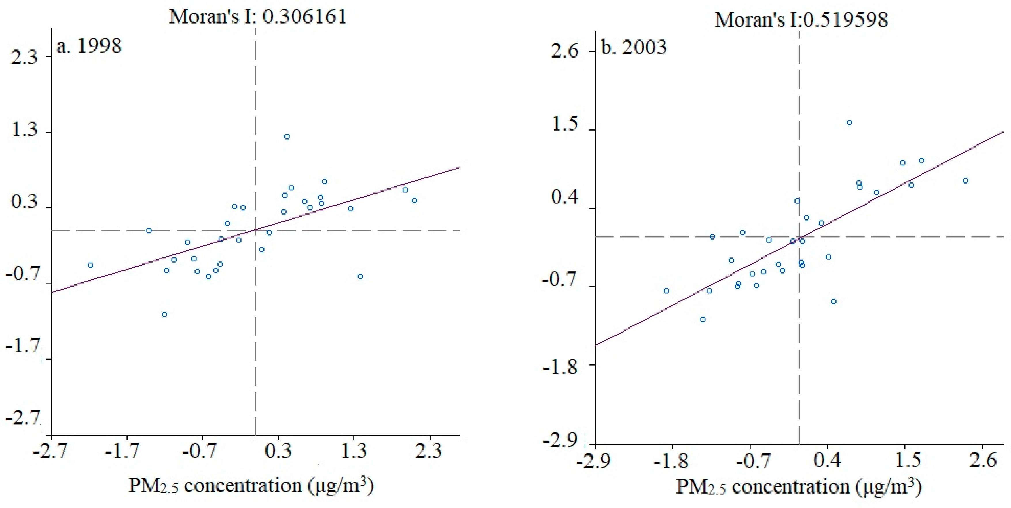
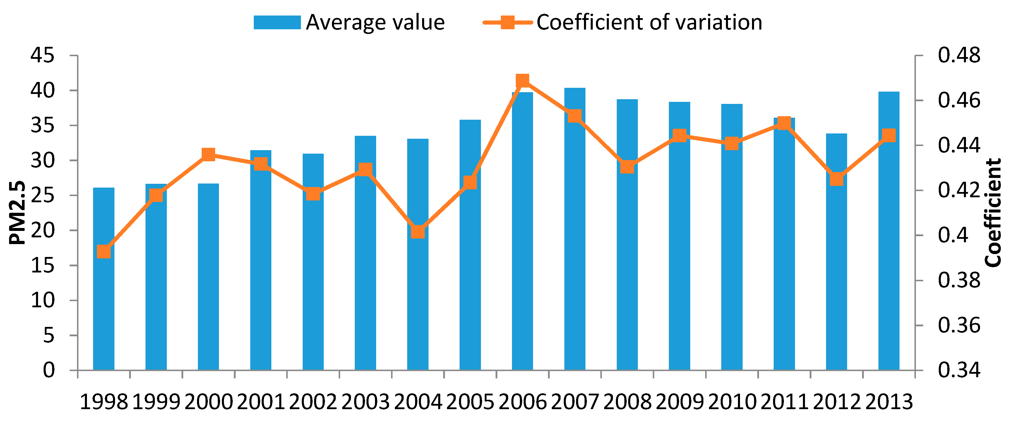
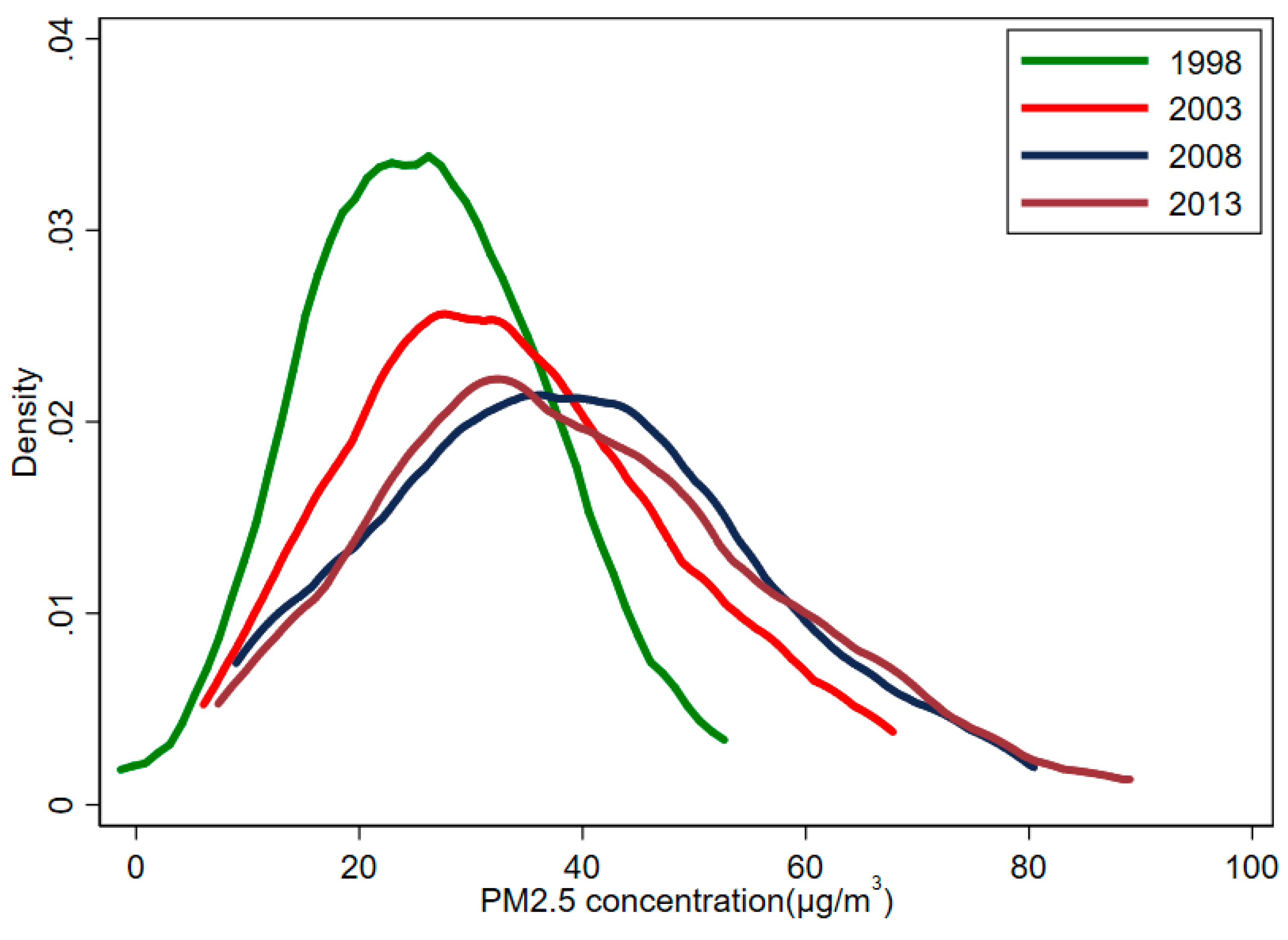
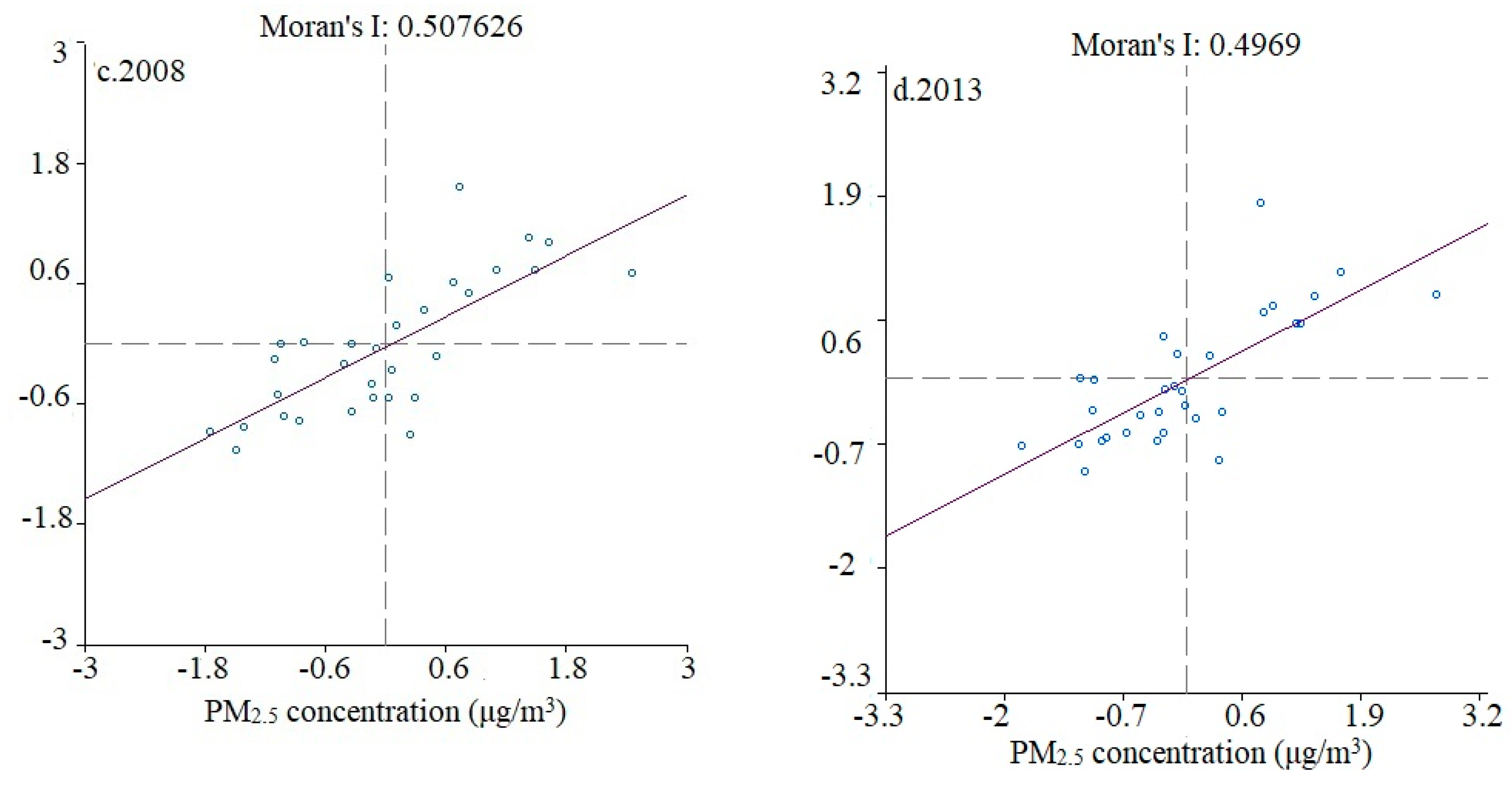
We have used the exploratory spatial data analysis method to examine the spatial autocorrelation of PM_2.5 pollution in 31 provinces in China between 1998 and 2013 and further used the SDM model to empirically investigate the impact of socioeconomic factors on haze pollution. In this section, we summarize our conclusions and make policy recommendations.

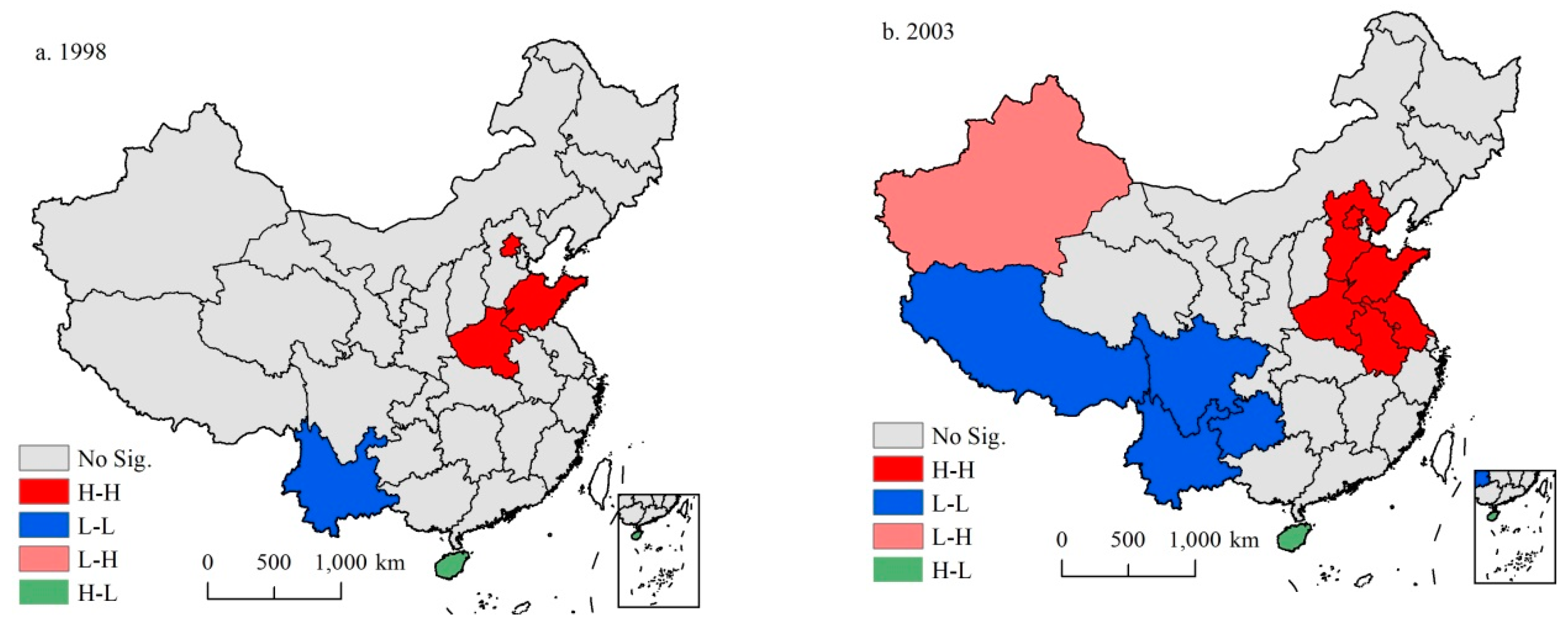
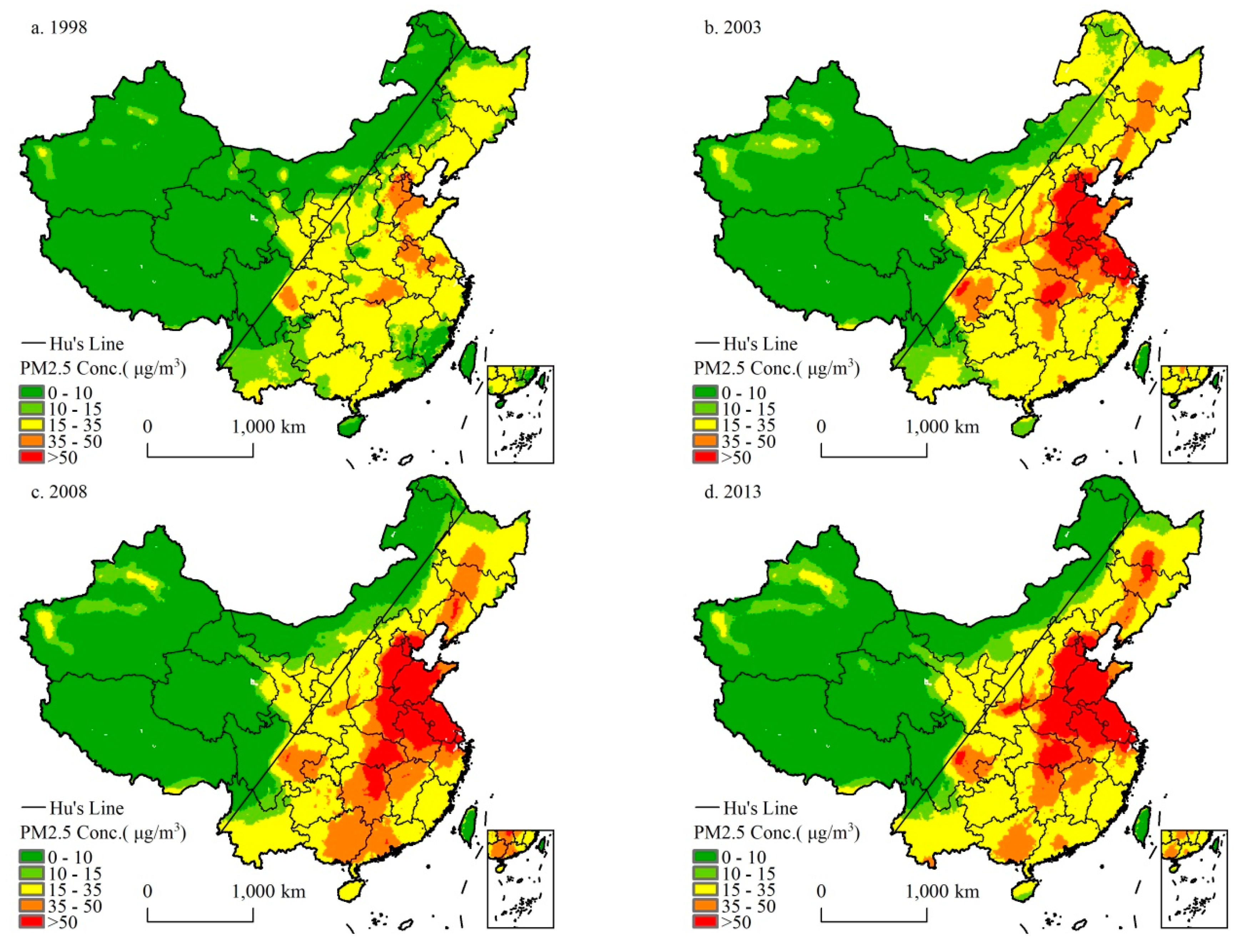
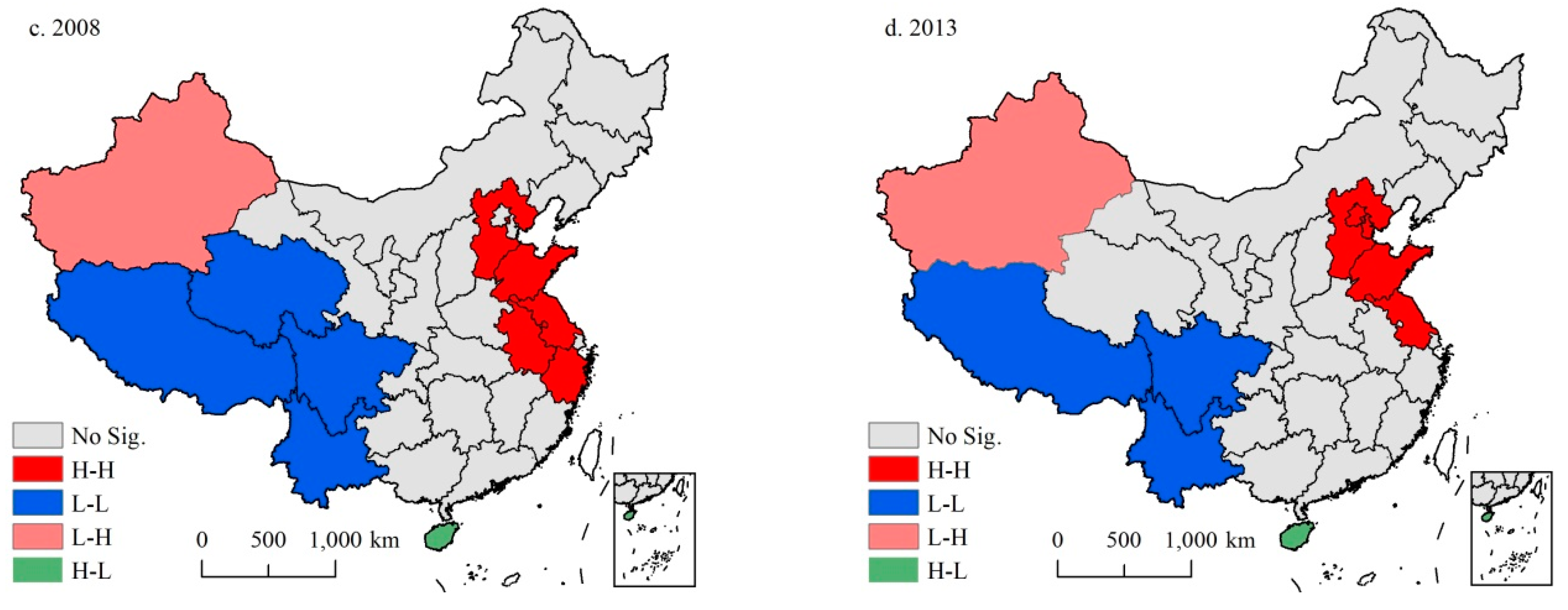
There is a significant spatial clustering characteristic of PM_2.5 pollution in China, i.e., high PM_2.5 polluted areas are adjacent to other high polluted areas, and low PM_2.5 polluted areas are adjacent to other low PM_2.5 polluted areas. The results show that the regions with high PM_2.5 concentrations are distributed in the Jing-Jin-Ji area in the north of China, the Henan province in central China, and the Shandong, Jiangsu, and Anhui provinces in eastern China. Considering the difference in PM_2.5 pollution level and the characteristics of agglomeration, the government should implement a differentiated regional pollution control strategy. For the Central and Eastern regions where high PM_2.5 concentrations are found, it should further strengthen comprehensive management to reduce pollution emissions. For the western regions with less haze pollution, it should raise the entry threshold for high pollution industry to prevent the risk of pollution shifted from east to west.

We found a significant positive spillover effect in China’s regional haze pollution. The increase of PM_2.5 concentration in neighboring areas will aggravate haze pollution in the region. To reduce the spatial effects of air pollution, it is necessary to strengthen haze control cooperation between provincial governments. The government should establish PM_2.5 pollution joint prevention, control, supervision, and coordination mechanism at the regional level, which transfers haze pollution control from local governance to regional integrated governance. Due to the “externality” of haze pollution control, cross-regional ecological compensation mechanism should be put in place to motivate participants to effectively implement cross-regional collaborative governance tasks.

Spatial econometric analysis results show that there is a significant N-shaped EKC curve between PM_2.5 pollution and economic growth. Some provinces are still to the left of the second inflection point where haze pollution will increase with economic growth. The decoupling phase between haze pollution and economic growth in China has not yet come. Most of the regions will be in a phase of simultaneous increase in pollution and economic growth in the coming period. The government should implement stricter environmental regulation measures to realize the decoupling between haze pollution and economic growth as soon as possible.

Population density, not surprisingly, has strong influences on PM_2.5 pollution. The higher the population density, the greater the demand for housing, home appliance, and motor vehicles, resulting in more energy consumption. Increased pollution emissions come not from these demands, from manufacturing, and also from traffic congestion. The government should attach great importance to the influence of population agglomeration on the quality of atmospheric environment. Raising the share of public transportation, the efficiency of resource use, and the sharing of pollution control and emission reduction facilities are essential measures to mitigate PM_2.5 pollution in high-density population areas.

Industrial structure also affects PM_2.5 concentration. Significant pollution results from secondary industry, especially heavy industry such as iron and steel, cement, etc. High-polluting industries emit large amounts of small particulate matter as well as other pollutants. As a result, one effective measure to reduce PM_2.5 pollution is to adjust and optimize industrial structure. In a country with coal as the main energy source, more needs to be done to diversify energy sources and reduce dependence on coal by increasing the number of renewable and clean energy sources such as wind and solar energy. Government departments should also strengthen policy guidance for cleaner production, energy conservation, and more recycling. In addition, the government needs to provide financial and technical support and encourage human talent for resource conservation and environmental protection.

In short, this study explores the dependence of PM_2.5 concentrations on economic activity and population density and provides a comprehensive insight into the economic mechanism of haze pollution in China. Furthermore, we reach policy conclusions based on our results and put forward ideas on controlling haze pollution. One of the limitations of our study is that the spatial unit analyzed is a province, a relatively large region. Given the development differences and the internal diversity in a single province, future research should identify the mechanisms generating PM_2.5 based on smaller scales in China, such as at the city and county level. As a complex air pollution phenomenon, PM_2.5 is affected by both climatic factors and human factors. Therefore, an estimation model including both anthropogenic factors and natural factors may be helpful in better understanding the mechanism of PM_2.5 formation in future research.

References

1. Pope, C.A. Review: Epidemiological Basis for Particulate Air Pollution Health Standards. Aerosol Sci. Technol. 2000, 32, 4–14. [Google Scholar] [CrossRef]
2. Hu, H.; Dailey, A.B.; Kan, H.; Xu, X. The effect of atmospheric particulate matter on survival of breast cancer among US females. Breast Cancer Res. Treat. 2013, 139, 217–226. [Google Scholar] [CrossRef] [PubMed]
3. Lelieveld, J.; Evans, J.S.; Fnais, M.; Giannadaki, D.; Pozzer, A. The contribution of outdoor air pollution sources to premature mortality on a global scale. Nature 2015, 525, 367–371. [Google Scholar] [CrossRef] [PubMed]
4. Qin, R.X.; Xiao, C.; Zhu, Y.; Li, J.; Yang, J.; Gu, S.; Xia, J.; Su, B.; Liu, Q.; Woodward, A. The interactive effects between high temperature and air pollution on mortality: A time-series analysis in Hefei, China. Sci. Total Environ. 2017, 575, 1530–1537. [Google Scholar] [CrossRef] [PubMed]
5. Chen, Z.; Wang, J.; Ma, G.; Zhang, Y. China tackles the health effects of air pollution. Lancet 2013, 382, 1959–1960. [Google Scholar] [CrossRef]
6. The World Bank. The Cost of Air Pollution; The World Bank: Washington, DC, USA, 2017. [Google Scholar]
7. Sampson, P.D.; Richards, M.; Szpiro, A.A.; Bergen, S.; Sheppard, L.; Larson, T.V.; Kaufman, J.D. A regionalized national universal kriging model using Partial Least Squares regression for estimating annual PM2.5 concentrations in epidemiology. Atmos. Environ. 2013, 75, 383–392. [Google Scholar] [CrossRef] [PubMed]
8. Zhang, X.; Zhang, X.; Chen, X. Happiness in the air: How does a dirty sky affect mental health and subjective well-being? J. Environ. Econ. Manag. 2017, 85, 81–94. [Google Scholar] [CrossRef] [PubMed]
9. Chen, Y.; Ebenstein, A.; Greenstone, M.; Li, H. Evidence on the impact of sustained exposure to air pollution on life expectancy from China’s Huai River policy. Proc. Natl. Acad. Sci. USA 2013, 110, 12936–12941. [Google Scholar] [CrossRef] [PubMed]
10. Wang, Y.; Zhang, R.; Saravanan, R. Asian pollution climatically modulates mid-latitude cyclones following hierarchical modelling and observational analysis. Nat. Commun. 2014, 5, 3098. [Google Scholar] [CrossRef] [PubMed]
11. Cao, J. Pollution status and control strategies of PM2.5 in China. J. Earth Environ. 2012, 3, 1030–1036. [Google Scholar]
12. Hu, J.; Ying, Q.; Wang, Y.; Zhang, H. Characterizing multi-pollutant air pollution in China: Comparison of three air quality indices. Environ. Int. 2015, 84, 17–25. [Google Scholar] [CrossRef] [PubMed]
13. China’s Ministry of Environmental Protection. Ambient Air Quality Standards GB3095-2012; China’s Ministry of Environmental Protection: Beijing, China, 2012. (In Chinese)
14. Huang, B.; Liu, M.; Ren, Z.; Bi, X.; Zhang, G.; Sheng, G.; Fu, J. Chemical composition, diurnal variation and sources of PM2.5 at two industrial sites of South China. Atmos. Pollut. Res. 2013, 4, 298–305. [Google Scholar] [CrossRef]
15. Chang, S.Y. The Characteristics of PM2.5 and Its Chemical Compositions between Different Prevailing Wind Patterns in Guangzhou. Aerosol Air Qual. Res. 2013, 13, 1373–1383. [Google Scholar] [CrossRef]
16. Li, J.; Song, Y.; Mao, Y.; Mao, Z.; Wu, Y.; Li, M.; Huang, X.; He, Q.; Hu, M. Chemical characteristics and source apportionment of PM2.5 during the harvest season in eastern China’s agricultural regions. Atmos. Environ. 2014, 92, 442–448. [Google Scholar] [CrossRef]
17. Zhang, Y.L.; Cao, F. Fine particulate matter (PM2.5) in China at a city level. Sci. Rep. 2015, 5, 14884. [Google Scholar] [CrossRef] [PubMed]
18. Wang, S.; Zhou, C.; Wang, Z.; Feng, K.; Hubacek, K. The characteristics and drivers of fine particulate matter (PM2.5) distribution in China. J. Clean. Prod. 2017, 142, 1800–1809. [Google Scholar] [CrossRef]
19. Grossman, G.; Krueger, A.B. Economic Growth and the Environment. Q. J. Econ. 1995, 110, 353–377. [Google Scholar] [CrossRef]
20. Ben Nasr, A.; Gupta, R.; Sato, J.R. Is there an Environmental Kuznets Curve for South Africa? A co-summability approach using a century of data. Energy Econ. 2015, 52, 136–141. [Google Scholar] [CrossRef]
21. Lau, L.-S.; Choong, C.-K.; Eng, Y.-K. Investigation of the environmental Kuznets curve for carbon emissions in Malaysia: Do foreign direct investment and trade matter? Energy Policy 2014, 68, 490–497. [Google Scholar] [CrossRef]
22. Wang, Y.; Zhang, C.; Lu, A.; Li, L.; He, Y.; ToJo, J.; Zhu, X. A disaggregated analysis of the environmental Kuznets curve for industrial CO2 emissions in China. Appl. Energy 2017, 190, 172–180. [Google Scholar] [CrossRef]
23. Fosten, J.; Morley, B.; Taylor, T. Dynamic misspecification in the environmental Kuznets curve: Evidence from CO2 and SO2 emissions in the United Kingdom. Ecol. Econ. 2012, 76, 25–33. [Google Scholar] [CrossRef]
24. Bölük, G.; Mert, M. The renewable energy, growth and environmental Kuznets curve in Turkey: An ARDL approach. Renew. Sustain. Energy Rev. 2015, 52, 587–595. [Google Scholar] [CrossRef]
25. Liddle, B. What are the carbon emissions elasticities for income and population? Bridging STIRPAT and EKC via robust heterogeneous panel estimates. Glob. Environ. Chang. 2015, 31, 62–73. [Google Scholar] [CrossRef]
26. Özokcu, S.; Özdemir, Ö. Economic growth, energy, and environmental Kuznets curve. Renew. Sustain. Energy Rev. 2017, 72, 639–647. [Google Scholar] [CrossRef]
27. Apergis, N.; Ozturk, I. Testing Environmental Kuznets Curve hypothesis in Asian countries. Ecol. Indic. 2015, 52, 16–22. [Google Scholar] [CrossRef]
28. Lin, C.-Y.C.; Liscow, Z.D. Endogeneity in the environmental Kuznets curve: An instrumental variables approach. Am. J. Agric. Econ. 2012, 95, 268–274. [Google Scholar] [CrossRef]
29. Fodha, M.; Zaghdoud, O. Economic growth and pollutant emissions in Tunisia: An empirical analysis of the environmental Kuznets curve. Energy Policy 2010, 38, 1150–1156. [Google Scholar] [CrossRef]
30. Wang, Z.; Bao, Y.; Wen, Z.; Tan, Q. Analysis of relationship between Beijing’s environment and development based on Environmental Kuznets Curve. Ecol. Indic. 2016, 67, 474–483. [Google Scholar] [CrossRef]
31. Khan, S.A.R.; Zaman, K.; Zhang, Y. The relationship between energy-resource depletion, climate change, health resources and the environmental Kuznets curve: Evidence from the panel of selected developed countries. Renew. Sustain. Energy Rev. 2016, 62, 468–477. [Google Scholar] [CrossRef]
32. Akbostancı, E.; Türüt-Aşık, S.; Tunç, G.İ. The relationship between income and environment in Turkey: Is there an environmental Kuznets curve? Energy Policy 2009, 37, 861–867. [Google Scholar] [CrossRef]
33. Kang, Y.-Q.; Zhao, T.; Yang, Y.-Y. Environmental Kuznets curve for CO2 emissions in China: A spatial panel data approach. Ecol. Indic. 2016, 63, 231–239. [Google Scholar] [CrossRef]
34. Brajer, V.; Mead, R.W.; Xiao, F. Searching for an Environmental Kuznets Curve in China’s air pollution. China Econ. Rev. 2011, 22, 383–397. [Google Scholar] [CrossRef]
35. Kivyiro, P.; Arminen, H. Carbon dioxide emissions, energy consumption, economic growth, and foreign direct investment: Causality analysis for Sub-Saharan Africa. Energy 2014, 74, 595–606. [Google Scholar] [CrossRef]
36. Nasir, M.; Rehman, F.U. Environmental Kuznets Curve for carbon emissions in Pakistan: An empirical investigation. Energy Policy 2011, 39, 1857–1864. [Google Scholar] [CrossRef]
37. Luo, K.; Li, G.; Fang, C.; Sun, S. PM2.5 mitigation in China: Socioeconomic determinants of concentrations and differential control policies. J. Environ. Manag. 2018, 213, 47–55. [Google Scholar] [CrossRef] [PubMed]
38. Hao, Y.; Liu, Y.-M. The influential factors of urban PM2.5 concentrations in China: A spatial econometric analysis. J. Clean. Prod. 2016, 112, 1443–1453. [Google Scholar] [CrossRef]
39. Li, M.; Li, C.; Zhang, M. Exploring the spatial spillover effects of industrialization and urbanization factors on pollutants emissions in China’s Huang-Huai-Hai region. J. Clean. Prod. 2018, 195, 154–162. [Google Scholar] [CrossRef]
40. Han, L.; Zhou, W.; Pickett, S.T.A.; Li, W.; Li, L. An optimum city size? The scaling relationship for urban population and fine particulate (PM2.5) concentration. Environ. Pollut. 2016, 208, 96–101. [Google Scholar] [CrossRef] [PubMed]
41. Fang, C.; Liu, H.; Li, G.; Sun, D.; Miao, Z. Estimating the Impact of Urbanization on Air Quality in China Using Spatial Regression Models. Sustainability 2015, 7, 15570–15592. [Google Scholar] [CrossRef]
42. Ma, Y.-R.; Ji, Q.; Fan, Y. Spatial linkage analysis of the impact of regional economic activities on PM2.5 pollution in China. J. Clean. Prod. 2016, 139, 1157–1167. [Google Scholar] [CrossRef]
43. Li, G.; Fang, C.; Wang, S.; Sun, C. The effect of economic growth, urbanization, and industrialization on fine particulate matter (PM2.5) concentrations in China. Environ. Sci. Technol. 2016, 50, 11452–11459. [Google Scholar] [CrossRef] [PubMed]
44. Xu, B.; Lin, B. Regional differences of pollution emissions in China: Contributing factors and mitigation strategies. J. Clean. Prod. 2016, 112, 1454–1463. [Google Scholar] [CrossRef]
45. Du, Y.; Sun, T.; Peng, J.; Fang, K.; Liu, Y.; Yang, Y.; Wang, Y. Direct and spillover effects of urbanization on PM2.5 concentrations in China’s top three urban agglomerations. J. Clean. Prod. 2018, 190, 72–83. [Google Scholar] [CrossRef]
46. Wu, H.X. The Chinese GDP growth rate puzzle: How fast has the Chinese economy grown? Asian Econ. Pap. 2007, 6, 1–23. [Google Scholar] [CrossRef]
47. Movshuk, O. The reliability of China’s growth figures: A survey of recent statistical controversies. J. Econ. Study Northeast Asia 2002, 4, 31–45. [Google Scholar]
48. Henderson, J.; Storeygard, V.A.; Weil, D.N. Measuring economic growth from outer space. Am. Econ. Rev. 2012, 102, 994–1028. [Google Scholar] [CrossRef] [PubMed]
49. Henderson, J.; Squires, T.; Storeygard, A.; Weil, D. The global distribution of economic activity: Nature, history, and the role of trade. Q. J. Econ. 2017, 133, 357–406. [Google Scholar]
50. Hodler, R.; Raschky, P.A. Regional favoritism. Q. J. Econ. 2014, 129, 995–1033. [Google Scholar] [CrossRef]
51. Sutton, P.C.; Costanza, R. Global estimates of market and non-market values derived from nighttime satellite imagery, land cover, and ecosystem service valuation. Ecol. Econ. 2002, 41, 509–527. [Google Scholar] [CrossRef]
52. Anselin, L. Local Indicators of Spatial Association-LISA. Geogr. Anal. 1995, 27, 93–115. [Google Scholar] [CrossRef]
53. Lesage, J.; Pace, R.K. Introduction to Spatial Econometrics; CRC Press: Boca Raton, FL, USA, 2009; pp. 137–182. [Google Scholar]
54. Anselin, L.; Bera, A.K.; Florax, R.; Yoon, M. Simple Diagnostic Tests for Spatial Dependence. Reg. Sci. Urban Econ. 1996, 26, 77–104. [Google Scholar] [CrossRef]
55. Van Donkelaar, A.; Martin, R.; Brauer, M.; L Boys, B. Use of Satellite Observations for Long-Term Exposure Assessment of Global Concentrations of Fine Particulate Matter. Environ. Health Perspect. 2014, 123, 135. [Google Scholar] [CrossRef] [PubMed]
56. Liu, Z.; He, C.; Zhang, Q.; Huang, Q.; Yang, Y. Extracting the dynamics of urban expansion in China using DMSP-OLS nighttime light data from 1992 to 2008. Landsc. Urban Plan. 2012, 106, 62–72. [Google Scholar] [CrossRef]
57. Guan, D.; Su, X.; Zhang, Q.; P Peters, G.; Liu, Z.; Lei, Y.; He, K. The socioeconomic drivers of China’s primary PM2.5 emissions. Environ. Res. Lett. 2014, 9, 024010. [Google Scholar] [CrossRef]
Figure 1. The distribution of PM2.5 concentration in China (1998, 2003, 2008, 2013).
Sustainability 11 01201 g001
Figure 2. Average and variation coefficient of Chinese PM2.5 concentration (1998–2013).
Sustainability 11 01201 g002
Figure 3. Kernel densities of PM2.5 concentration at the provincial level: 1998, 2003, 2008, and 2013.
Sustainability 11 01201 g003
Figure 4. Moran scatter plots of PM2.5 concentration in 31 Chinese provinces.
Sustainability 11 01201 g004aSustainability 11 01201 g004b
Figure 5. LISA cluster map of PM2.5 concentration in China in 1998, 2003, 2008, and 2013.
Sustainability 11 01201 g005aSustainability 11 01201 g005b