Measuring Community Greening Merging Multi-Source Geo-Data


Abstract
1. Introduction
2. Data and Methods
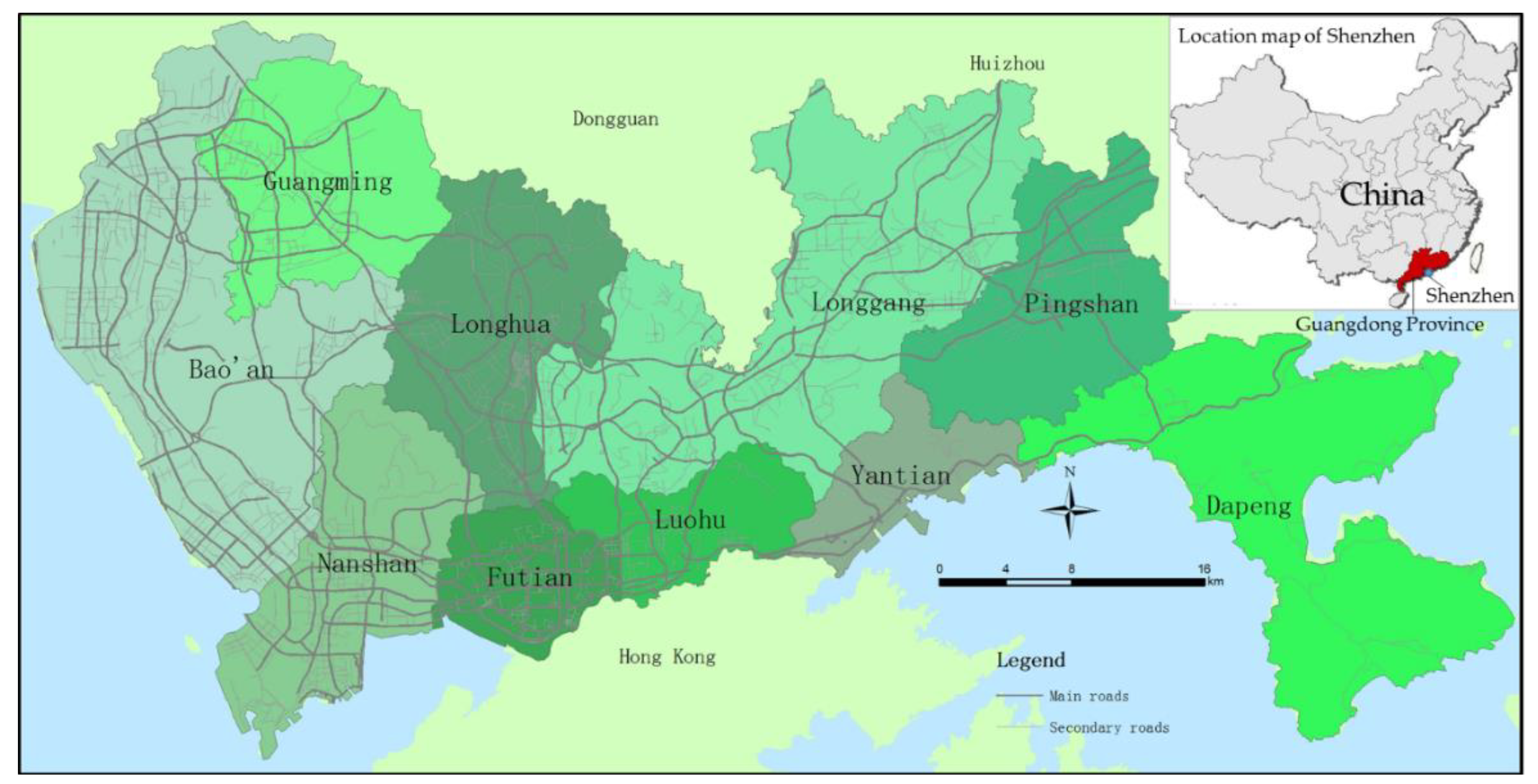
2.1. Case Selection
2.2. Residential Unit and Type Identification
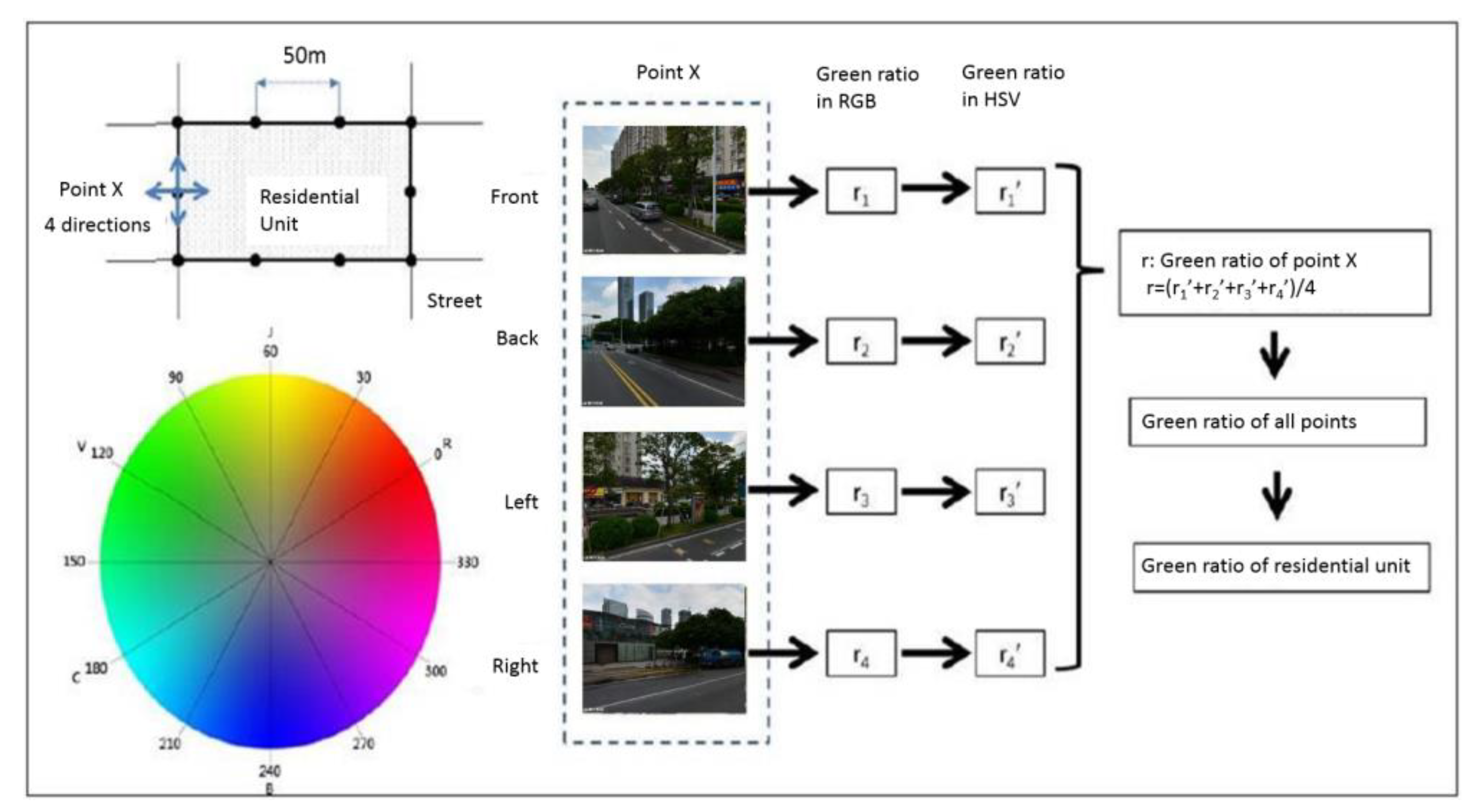
2.3. Calculation of Three Greening Indicators
2.4. Database Establishment and Statistical Analysis
3. Results
3.1. Overall Greening Level and Correlation amongst Different Indicators
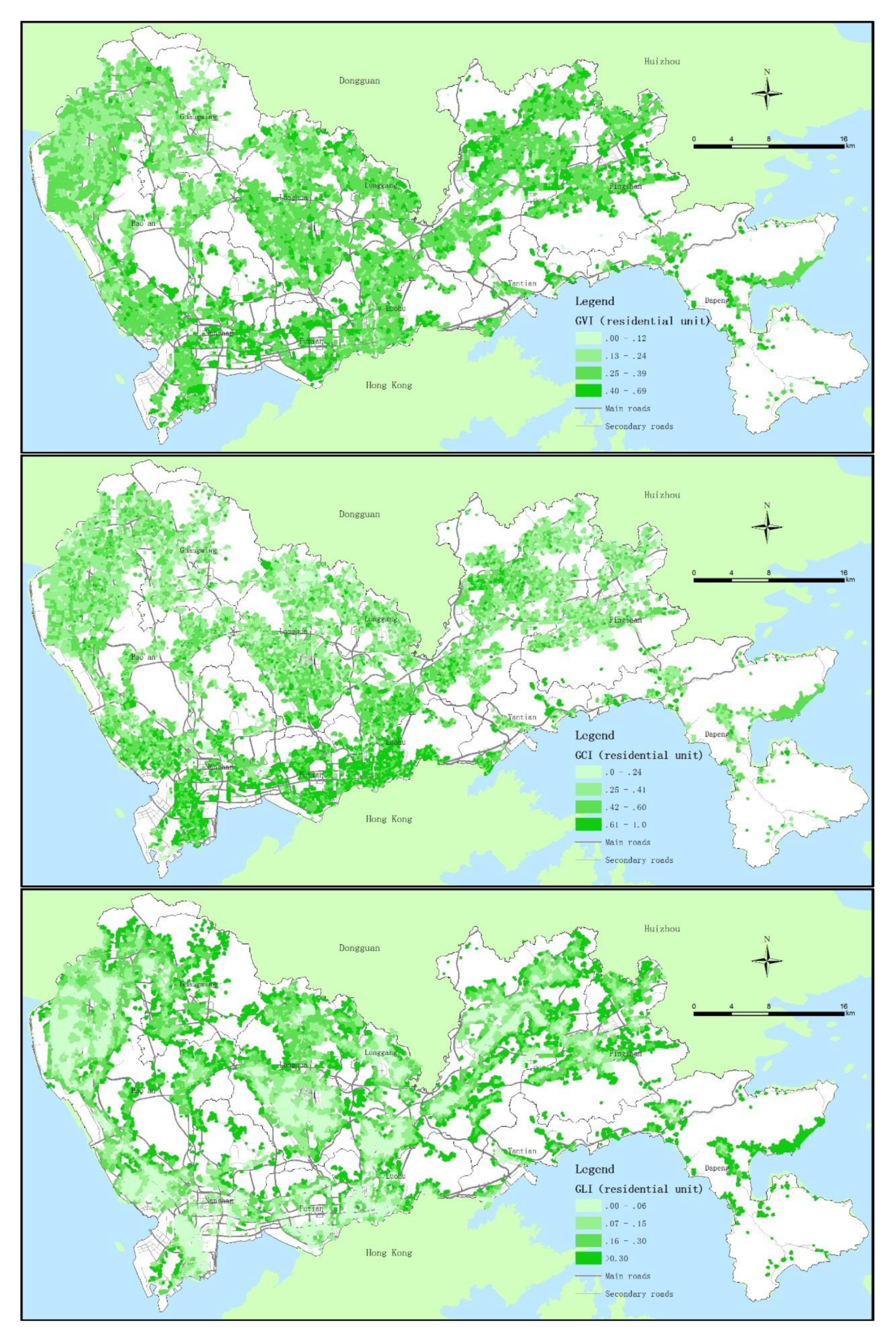
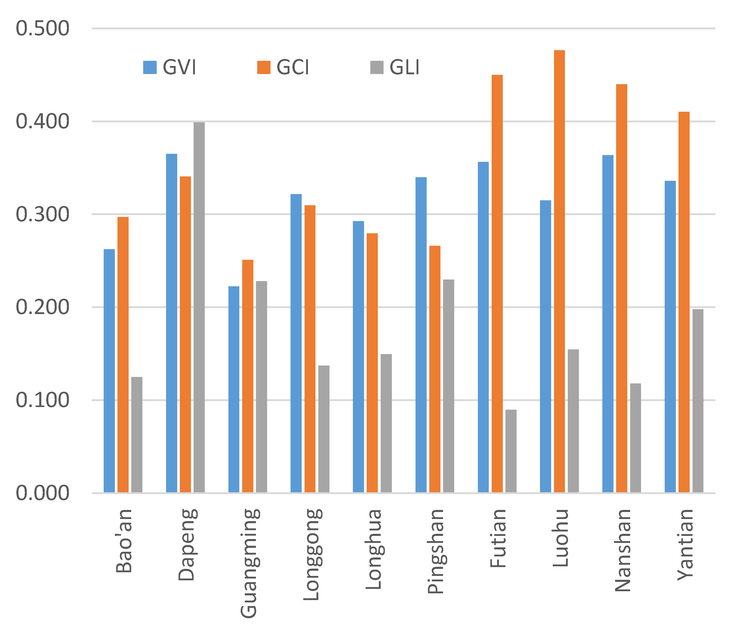
3.2. Spatial Differences of Residential Greening
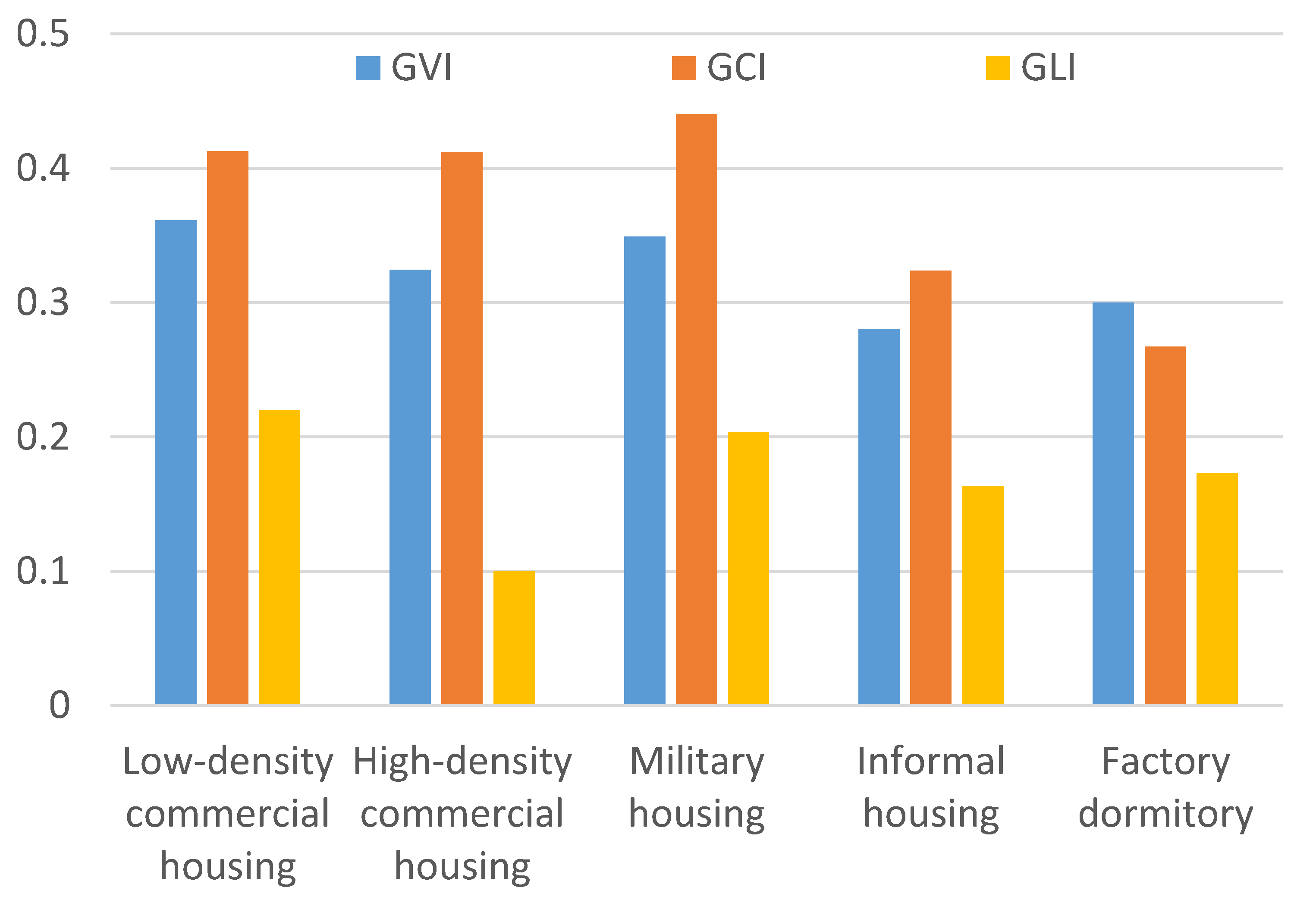
3.3. Greening Differences amongst Different Types of Residential Units
3.4. Factors Affecting Residential Greening
4. Discussions and Conclusions
Author Contributions
Funding
Acknowledgments
Conflicts of Interest
References
- Koohsari, M.J.; Mavoa, S.; Villanueva, K.; Sugiyama, T.; Badland, H.; Kaczynski, A.T.; Owen, N.; Giles-Corti, B. Public open space, physical activity, urban design and public health: Concepts, methods and research agenda. Health Place 2015, 33, 75–82. [Google Scholar] [CrossRef]
- Ward Thompson, C.; Roe, J.; Aspinall, P.; Mitchell, R.; Clow, A.; Miller, D. More green space is linked to less stress in deprived communities: Evidence from salivary cortisol patterns. Landsc. Urban Plan. 2012, 105, 221–229. [Google Scholar] [CrossRef]
- Chen, Y.; Liu, X.; Gao, W.; Wang, R.Y.; Li, Y.; Tu, W. Emerging social media data on measuring urban park use. Urban For. Urban Green. 2018, 31, 130–141. [Google Scholar] [CrossRef]
- Larson, L.R.; Keith, S.J.; Fernandez, M.; Hallo, J.C.; Shafer, C.S.; Jennings, V. Ecosystem services and urban greenways: What’s the public’s perspective? Ecosyst. Serv. 2016, 22, 111–116. [Google Scholar] [CrossRef]
- Bertram, C.; Rehdanz, K. The role of urban green space for human well-being. Ecol. Econ. 2015, 120, 139–152. [Google Scholar] [CrossRef]
- Goličnik Marušić, B. Discrepancy between likely and actual occupancies of urban outdoor places. Urban For. Urban Green. 2016, 18, 151–162. [Google Scholar] [CrossRef]
- Parker, J.D.; Akinbami, L.J.; Woodruff, T.J. Air Pollution and Childhood Respiratory Allergies in the United States. Environ. Health Perspect. 2009, 117, 140–147. [Google Scholar] [CrossRef]
- Li, X.; Zhang, C.; Li, W.; Kuzovkina, Y.A.; Weiner, D. Who lives in greener neighborhoods? The distribution of street greenery and its association with residents’ socioeconomic conditions in Hartford, Connecticut, USA. Urban For. Urban Green. 2015, 14, 751–759. [Google Scholar] [CrossRef]
- Pham, T.-T.-H.; Apparicio, P.; Landry, S.; Lewnard, J. Disentangling the effects of urban form and socio-demographic context on street tree cover: A multi-level analysis from Montréal. Landsc. Urban Plan. 2017, 157, 422–433. [Google Scholar] [CrossRef]
- Harvey, C.; Aultman-Hall, L.; Hurley, S.E.; Troy, A. Effects of skeletal streetscape design on perceived safety. Landsc. Urban Plan. 2015, 142, 18–28. [Google Scholar] [CrossRef]
- Lin, Y.H.; Tsai, C.C.; Sullivan, W.C.; Chang, P.J.; Chang, C.Y. Does awareness effect the restorative function and perception of street trees? Front. Psychol. 2014, 5, 906. [Google Scholar] [CrossRef]
- Ying-shu, Y.; Jin-hui, P.; De-qiong, S.; Hong-can, Z.; Yan-ning, H. Advance in Evaluation Index System of Green Land Plan of Urban Road. J. Northwest For. Univ. 2007, 193–197. [Google Scholar]
- Xiang, Z.; Zhang, X.; Longbin, H.E.; Hui, Z. Equity Assessment on Urban Green Space Pattern Based on Human Behavior Scale and Its Optimization Strategy: A Case Study in Shenzhen. Acta Sci. Nat. Univ. Pekin. 2013, 49, 892–898. [Google Scholar]
- Yunfeng, H.U.; Zhao, G.; Zhang, Y. Analysis of Spatial and Temporal Dynamics of Green Coverage and Vegetation Greenness in Beijing. J. Geo-Inf. Sci. 2018. [Google Scholar] [CrossRef]
- Aoki, Y. Trends of Researches on Visual Geenery since 1974 in Japan. Environ. Inf. Sci. 2006, 34, 46–49. [Google Scholar]
- Yu, S.; Yu, B.; Song, W.; Wu, B.; Zhou, J.; Huang, Y.; Wu, J.; Zhao, F.; Mao, W. View-based greenery: A three-dimensional assessment of city buildings’ green visibility using Floor Green View Index. Landsc. Urban Plan. 2016, 152, 13–26. [Google Scholar] [CrossRef]
- Tennessen, C.M.; Cimprich, B. Views to nature: Effects on attention. J. Environ. Psychol. 1995, 15, 77–85. [Google Scholar] [CrossRef]
- Li, X.; Zhang, C.; Li, W.; Ricard, R.; Meng, Q.; Zhang, W. Assessing street-level urban greenery using Google Street View and a modified green view index. Urban For. Urban Green. 2015, 14, 675–685. [Google Scholar] [CrossRef]
- Jiang, B.; Larsen, L.; Deal, B.; Sullivan, W.C. A dose–response curve describing the relationship between tree cover density and landscape preference. Landsc. Urban Plan. 2015, 139, 16–25. [Google Scholar] [CrossRef]
- Zhao, Q.; Tang, H.; Wei, D.; Qian, W. Spatial visibility of green areas of urban greenway using the green appearance percentage. J. Zhejiang A F Univ. 2016, 33, 288–294. [Google Scholar]
- Long, Y.; Liu, L. How green are the streets? An analysis for central areas of Chinese cities using Tencent Street View. PLoS ONE 2017, 12, e0171110. [Google Scholar]
- Rai, A. Designing Green Stormwater Infrastructure for Hydrologic and Human Benefits: An Image Based Machine Learning Approach. Master’s Thesis, University of Illinois, Champaign, IL, USA, 2013. [Google Scholar]
- Bureau, S.U.M. Shenzhen National Land Greening White Paper (2016–2017); Shenzhen City Administration: Shenzhen, China, 2018.
- Che, X.; English, A.; Jia, L.; Chen, Y.D. Improving the Effectiveness of Planning EIA (PEIA) in China: Integrating Planning and Assessment during the Preparation of Shenzhen’s Master Urban Plan. Environ. Impact Assess. Rev. 2011, 31, 561–571. [Google Scholar] [CrossRef]
- Tu, W.; Hu, Z.; Li, L.; Cao, J.; Jiang, J.; Li, Q.; Li, Q. Portraying Urban Functional Zones by Coupling Remote Sensing Imagery and Human Sensing Data. Remote Sens. 2018, 10, 141. [Google Scholar] [CrossRef]
- Wüstemann, H.; Kalisch, D.; Kolbe, J. Access to urban green space and environmental inequalities in Germany. Landsc. Urban Plan. 2017, 164, 124–131. [Google Scholar] [CrossRef]
- MPGS (Municipal People’s Government of Shenzhen). Shenzhen Urban Planning Standards and Guidelines; Shenzhen Municipal People’s Government: Shenzhen, China, 2013.
- Ewing, R.; Cervero, R. Travel and the Built Environment. J. Am. Plan. Assoc. 2010, 76, 265–294. [Google Scholar] [CrossRef]
- Yue, Y.; Zhuang, Y.; Yeh, A.G.O.; Xie, J.-Y.; Ma, C.-L.; Li, Q.-Q. Measurements of POI-based mixed use and their relationships with neighbourhood vibrancy. Int. J. Geogr. Inf. Sci. 2016, 31, 658–675. [Google Scholar] [CrossRef]
- Gupta, K.; Roy, A.; Luthra, K.; Maithani, S.; Mahavir. GIS based analysis for assessing the accessibility at hierarchical levels of urban green spaces. Urban For. Urban Green. 2016, 18, 198–211. [Google Scholar] [CrossRef]
- Richard, M.; Thomas, A.B.; Richardson, E.A. A comparison of green space indicators for epidemiological research. J. Epidemiol. Community Health 2011, 65, 853–858. [Google Scholar]
- Voorde, T.V.D. Spatially explicit urban green indicators for characterizing vegetation cover and public green space proximity: A case study on Brussels, Belgium. Int. J. Digit. Earth 2017, 10, 1–16. [Google Scholar] [CrossRef]
- Le Texier, M.; Schiel, K.; Caruso, G.; Arcaute, E. The provision of urban green space and its accessibility: Spatial data effects in Brussels. PLoS ONE 2018, 13, 1–17. [Google Scholar] [CrossRef]
- Cohen, D.A.; Han, B.; Nagel, C.J.; Harnik, P.; McKenzie, T.L.; Evenson, K.R.; Marsh, T.; Williamson, S.; Vaughan, C.; Katta, S. The First National Study of Neighborhood Parks: Implications for Physical Activity. Am. J. Prev. Med. 2016, 51, 419–426. [Google Scholar] [CrossRef]
- Tamosiunas, A.; Grazuleviciene, R.; Luksiene, D.; Dedele, A.; Reklaitiene, R.; Baceviciene, M.; Vencloviene, J. Accessibility and use of urban green spaces, and cardiovascular health: Findings from a Kaunas cohort study. Environ. Health 2014, 13, 1–11. [Google Scholar] [CrossRef]


| Type of Residential Unit | Number of Residential Units | Gross Residential Area (m2) |
|---|---|---|
| Informal housing | 3737 | 192,216,070 |
| High-density commercial housing | 4582 | 248,956,472 |
| Low-density commercial housing | 1202 | 36,327,790 |
| Military housing | 51 | 3,124,590 |
| Factory dormitory | 10,003 | 136,687,441 |
| Total | 19,575 | 617,312,363 |
| Indicator | GCI (Green Coverage Index) | GLI (Green Land Index) | GVI (Green View Index) |
|---|---|---|---|
| Full spelling | Green coverage index | Accessible public green land index | Green view index |
| Definition | An index to measure the green coverage of residential units | An index to measure public green land around the walking range of residents | An index to measure the visible greening of surrounding street space of residential area |
| Objection | Total amount of various green spaces, including residential parks, greening between houses, roof greening, canopy of large trees, etc. | Various public green lands including urban, theme, community and country parks, open space, mountainous parks | All green elements on street view, including trees, shrub, lawn, vertical greening, even painted green wall |
| Data source | High-resolution satellite remote sensing image data | Citywide land-use vector data from the planning agency | Street view photos collected from tencent street view map |
| Calculation | The proportion of the green coverage area within the land area of the residential unit | The ratio of various public green lands within the residential unit and 500 m buffer zone of the residential unit, to the total area | The ratio of the number of green pixels to the total number of pixels in street view photos |
| Variables | Mean Value | Standard Deviation | Maximum Value | Minimum Value |
|---|---|---|---|---|
| Parcel area (m2) | 24,786.75 | 34,286.35 | 787,620.81 | 2000.01 |
| Number of buildings in each unit | 35 | 84 | 3142 | 1 |
| Gross floor area (m2) | 52,038.56 | 70,226.51 | 1,106,262.79 | 1216.80 |
| Gross residential area (m2) | 36,714.03 | 60,994.06 | 990,345.75 | 1000.99 |
| Building density | 0.473 | 0.165 | 1.000 | 0.001 |
| Floor area ratio | 2.66 | 2.28 | 27.79 | 0.01 |
| GLI | 0.151 | 0.149 | 0.982 | 0.000 |
| GVI | 0.305 | 0.084 | 0.726 | 0.050 |
| GCI | 0.327 | 0.137 | 0.922 | 0.000 |
| Variable Types | Variables | GVI | GCI | GLI |
|---|---|---|---|---|
| Characteristics of residential units | Parcel area | 0.018 | −0.053 ** | −0.019 |
| Number of buildings | −0.073 ** | −0.030 * | −0.016 | |
| Building density | −0.179 ** | −0.151 ** | −0.106 ** | |
| Floor area ratio | −0.043 ** | −0.071 ** | −0.051 ** | |
| Whether it is commercial housing (yes = 1) | 0.172 ** | 0.101 ** | 0.050 ** | |
| Whether it is a factory dormitory (yes = 1) | −0.088 ** | −0.154 ** | −0.026 | |
| Location | Whether it is in the original SEZ (yes = 1) | 0.363 ** | 0.273 ** | 0.312 ** |
| Distance from CBD | −0.195 ** | −0.067 ** | −0.324 ** | |
| Number of bus lines | −0.016 | 0.018 | −0.038 | |
| Surrounding environment | Whether it is backed by a mountain (yes = 1) | 0.032 | 0.011 | −0.006 |
| Whether it is facing water (yes = 1) | −0.061 * | −0.008 | −0.021 * | |
| Elevation | 0.274 ** | 0.053 ** | 0.260 ** | |
| Sample quantity | 14196 | 14196 | 14196 | |
| adj R2 | 0.195 | 0.319 | 0.265 | |
| F value | 287.7 | 553.3 | 426.1 |
© 2019 by the authors. Licensee MDPI, Basel, Switzerland. This article is an open access article distributed under the terms and conditions of the Creative Commons Attribution (CC BY) license (http://creativecommons.org/licenses/by/4.0/).
Share and Cite
Gu, W.; Chen, Y.; Dai, M. Measuring Community Greening Merging Multi-Source Geo-Data. Sustainability 2019, 11, 1104. https://doi.org/10.3390/su11041104
Gu W, Chen Y, Dai M. Measuring Community Greening Merging Multi-Source Geo-Data. Sustainability. 2019; 11(4):1104. https://doi.org/10.3390/su11041104
Chicago/Turabian StyleGu, Weiying, Yiyong Chen, and Muye Dai. 2019. "Measuring Community Greening Merging Multi-Source Geo-Data" Sustainability 11, no. 4: 1104. https://doi.org/10.3390/su11041104
APA StyleGu, W., Chen, Y., & Dai, M. (2019). Measuring Community Greening Merging Multi-Source Geo-Data. Sustainability, 11(4), 1104. https://doi.org/10.3390/su11041104