Multi-Criteria, Cost-Benefit, and Life-Cycle Analyses for Decision-Making to Support Responsible, Sustainable, and Alternative Tourism

Abstract

This paper combines the most popular tourism typologies or goals (i.e., RT, responsible tourism, to represent impact minimisation; ST, sustainable tourism, to represent welfare maximisation; AT, alternative tourism, to represent continuity maximisation) and decision-making methodologies (i.e., MCA, multi-criteria analysis; CBA, cost-benefit analysis; WLCA, weighted life-cycle assessment; MLCA, monetary life-cycle assessment) in a single dynamic framework to operationally match the former with the latter. Normative insights show that MCA and WLCA are most suitable for RT and AT, respectively, whereas CBA and MLCA are most suitable for ST. Management recommendations (i.e., if a wrong static instead of a right dynamic approach must be adopted due to a lack of data, once chosen a tourism typology or goal, ST is the best in terms of level, correlation and likelihood of errors) are provided, and policy recommendations (i.e., if a right dynamic approach is adopted, in choosing among tourism typologies or goals, AT is the best in terms of precaution, ST is the best in terms of correlation, and RT is the best in terms of risk of investments) are suggested for a case study characterized by negative environmental and cultural dynamics. Positive insights show that two and many papers have applied WLCA and MLCA, respectively, to RT, but they did not account for cultural features; many papers have applied CBA to ST, but only one paper applied MLCA; few and no papers have applied MCA and WLCA, respectively, to AT.

1. Introduction

Tourism typologies or goals such as “sustainable” tourism are meaningless if they do not provide indicators that can assess current or future scenarios and support the development of policies or projects. However, definitions and objectives drive the choice among the decision-making methodologies and indicators. Moreover, indicators depend on the definitions to be applied once a suitable decision-making methodology has been chosen. Finally, the policies or projects to be evaluated depend on the targets, and must be measured by indicators that are suitable for those objectives. Note that any approach to policies or projects requires a proper matching between definitions, goals, assessment methodologies, and indicators, whether in the context of the cooperative tools on a project basis that were endorsed by [1], the voluntary tools on a project basis supported by [2], the financing tools on a project basis for social responsibility supported by [3], or the market-based policies suggested by [4].

The purpose of the present study was to balance the perspectives of politicians [5] and researchers [6] by referring to the main concepts of sustainability science (i.e., impacts and continuity) and the main concepts of development politics (i.e., weak sustainability, a-growth, and strong sustainability) in order to operationally match the most popular tourism typologies or goals (i.e., RT, responsible tourism, to represent impact minimisation; ST, sustainable tourism, to represent welfare maximisation; AT, alternative tourism, to represent continuity maximisation) with suitable indicators, appropriate decision-making methodologies (cost-benefit analysis, CBA; multi-criteria analysis, MCA; weighted life-cycle assessment, WLCA; and monetary life-cycle assessment, MLCA), and suitable policies or projects. In order to do so, I use static concepts such as the objectives to be achieved (i.e., economic, social, environmental, and cultural targets) rather than dynamic concepts such as systems to be managed. I do not espouse any firm theory, although corporate social responsibility turns out to be close to weak sustainability in terms of how it assumes a combination of profit maximization with public sensitivity [7]. In addition, I do not adopt any specific growth theory, and instead adopt a local or regional planning approach (i.e., economic, social, environmental, and cultural investments). I do not refer to any consumption theory, although ethical consumption is close to RT and AT in its assumption that the objective is to drive public interventions towards sustainability [8]. In particular, I will suggest which decision-making methodologies should be implemented to assess each tourism typology or goal. I will highlight which data are needed to apply the right methodology (i.e., WLCA > MCA if the goal is to minimise impacts; MLCA > CBA if the goal is to maximise welfare; WLCA > MCA if the goal is to maximise continuity), and I will stress which errors (i.e., excessive or insufficient investments in environment or culture) result from applying the wrong static methodology (e.g., due to a lack of data) (Section 4.1) by emphasizing the likelihood of, and the correlation between, errors in the allocation of investments between environment and culture (i.e., their dependence and cross-dependence on the estimated environmental and cultural dynamics, respectively). I will highlight differences in investments when alternative right dynamic decision-making methodologies are used (Section 4.2) by emphasizing the precautionary characteristics of investment decisions (i.e., larger investments in environment or culture, leading to a greater likelihood of environmental and cultural preservation), the risk of, and the correlation between, investment decisions (i.e., higher sensitivity and cross-sensitivity to the estimated environmental and cultural dynamics, respectively). I will also estimate the impacts of policies on these differences in investments by emphasizing precaution, risk and correlation. Note that I will perform empirical comparisons of investment decisions based on a case study in Northern Italy if these comparisons cannot be carried out theoretically. In other words, identifying tourism typologies and goals will let me refer to goals to formalize the tourism typologies (Section 2) and obtain normative insights, and will let me refer to typologies to sort papers that have applied alternative assessment methodologies in the context of previous research results (Section 5) and obtain positive insights. Similarly, matching the goals with the appropriate assessment methodologies and indicators (i.e., static vs. dynamic indicators, independent vs. inter-dependent variables) will let me better define the tourism typologies. For example, if CBA is applied where positive environmental and cultural dynamics are observed, then ST is implicitly chosen in terms of its smaller risk, the larger precautionary component of the investment decisions, and in terms of its smaller correlation with dynamic variables. In summary, the following management recommendations will be provided: if choices are driven by data availability, CBA applied to ST should be preferred to MCA applied to RT and AT in terms of level, correlation and likelihood of errors; errors for AT show higher level and correlation, but smaller likelihood than RT. Next, a case study in Northern Italy, characterized by negative environmental and cultural dynamics, will suggest the following policy recommendations: if choices are driven by investment characteristics, AT estimated by WLCA should be preferred in terms of precaution, RT estimated by WLCA should be preferred in terms of risk, and ST estimated by MLCA should be preferred in terms of correlation of investments; investments for RT and AT show the same correlation and risk.

Note that all three tourism typologies emphasize stakeholder participation, although to different extents, so that market prices, as summary assessments of potentially conflicting interests and perceptions, must be replaced by alternative valuation procedures. For example, the analytic hierarchy process can be used to estimate relative weights or statistics can be used to estimate demand functions, with both methods accounting for the most representative stakeholders. Moreover, ST is close to weak sustainability, whereas RT and AT are closer to a-growth and strong sustainability, respectively, although with different goals and indicators. Finally, all four pillars of the analysis (economic, social, environmental, and cultural features) can be assessed by properly fine-tuning the four decision-making methodologies, so issues do not force a specified matching between the tourism typology and the analytical method. For example, income distribution effects that characterize RT or poverty alleviation effects that characterize AT could be estimated by CBA.

2. Definitions and Goals

In this section, I will discuss the main scientific and political concepts that underlie my analysis. I assume that the development of tourism opportunities will include both planning and management. In this paper, I will focus on developing tools to support planning and management of both existing and new tourism resources. Note that different stakeholders could have different objectives that must be accounted for in the decision-making process [9].

In the scientific literature, sustainability refers to “social and ecological resilience” [10], and the impacts and continuity are crucial aspects. In contrast, the United Nations Commission on Environment and Development (the Brundtland Commission) introduced the concept of sustainable development in 1987: “development that meets the needs of the present without compromising the ability of future generations to meet their own needs”. In this context, two concepts are crucial [11]: priority should be given to the essential needs of the world’s poor (i.e., distributive justice in outcomes for current generations), and limitations imposed by the state of technology and social organization on the environment’s ability to meet present and future needs should be stressed (i.e., technological and social innovation should be limited to the currently or imminently available technologies and organizations). By reframing this concept, three main sustainability paradigms have been suggested in the policy literature [12]. By replacing “needs” with “welfare”, weak sustainability allows for natural resources to be depleted if this is compensated for by other resources (i.e., “development that allows the present generation to maximize its welfare without compromising the ability of future generations to maximize their own welfare”). By allowing for substitution between forms of capital to increase welfare, a-growth (i.e., an ecological and economic strategy based on indifference to or neutrality about economic levels and growth, with growth considered to be a non-robust and unreliable indicator of social welfare and progress) focuses on the many neglected non-market transactions (e.g., informal activities and relationships) and the many unpriced environmental effects. By aiming to preserve all separate species and resources, strong sustainability stresses that natural and physical or social capitals are complementary rather than interchangeable (i.e., “development that allows future generations to access to the same amount of natural resources and the same status of the environment as the current generation”).

Note that weak sustainability is consistent with an economic general equilibrium framework, whereas strong sustainability is consistent with an ecosystem services framework. Moreover, de-growth (i.e., an ecological and economic perspective based on a socially sustainable and equitable reduction, and eventually stabilization, of the materials and energy that a society extracts, processes, transports, distributes, consumes, and returns back to the environment as waste) is irrelevant in a context of planning a (new) tourist destination to improve economic and social indicators such as income and employment. Finally, a-growth is consistent with an economic general equilibrium framework, provided that prices reflect the rights of all stakeholders.

I have made three main contextual assumptions. First, I will focus on four pillars of tourism sustainability (i.e., k = eco, soc, env, and cul, respectively, to depict economic, social, environmental, and cultural features). Indeed, since the relative weights of the four pillars must be based on stakeholder preferences, possible sub-features should be combined into the four pillar features to allow reliable estimation of preferences. Note that air and water quality (i.e., pollution) belong to the stock variable Y_env together with the features of the natural environment that can be enjoyed, such as vegetation and wildlife (i.e., renewable resources), or land, beaches, and mountains (i.e., non-renewable resources). In contrast, historical and artistic monuments, dialects, traditions, arts, ceremonies, handicrafts, and museums are captured by the stock variable Y_cul together with the whole cultural heritage of the local community.

Second, environmental and cultural issues are affected over time by external factors that are not under the control of decision makers [13]. In particular, by defining the flow variables X_k(t) as a change over time (t) in stock variables Y_k(t) for pillar k, such that ∂Y(t)/∂t = X(t), I will refer to positive AR (1) (i.e., first-order autoregressive) dynamics to depict renewable resources (e.g., fish in a protected area), virtuous pollution reduction (e.g., a waste recycling system that improves behaviours), and cultural heritage (e.g., restored historical buildings, museums) for environmental and cultural issues, respectively:

X_k(t) = aX_k(t − 1) + η_k(t) such that X_k(T) = a^T X_k(0) + ∑ a^T−t η_k(t)

(1)

where a represents the influence of the variable X(t − 1), with a one-period time lag, on its current value X(t), where t represents the number of time periods since the start of the calculation; η represents unobservable random disturbances; T represents the planning and management horizon (in years); and 0 represents the start of the calculation period. In contrast, I refer to negative AR (1) dynamics to depict non-renewable resources (e.g., over-exploitation of a wild beach or mountain), vicious pollution reduction (e.g., a wastewater treatment plant that does not affect wasting behaviours), and cultural heritages (e.g., a commodification of traditional ceremonies or handicrafts) for environmental and cultural issues, respectively:

X_k(t) = a X_k(t − 1) − η_k(t) such that X_k(T) = a^T X_k(0) − ∑ a^T−t η_k(t)

(2)

Indeed, alternative dynamics such as a positive MA (1) (i.e., first-order moving average) or a negative MA (1) would require a choice for X_k(t) at each time t:

Positive: X_k(t) = η_k(t) + b η_k(t − 1) such that X_k(T) = η_k(T) + ∑ b^t X_k(t)

(3)

Negative: X_k(t) = η_k(t) − b η_k(t − 1) such that X_k(T) = η_k(T) − ∑ b^t X_k(t)

(4)

where b represents the influence of the disturbance η(t − 1) with a one-period time lag on the current value of the variable X(t), where t represents the number of time periods since the start of the calculation.

Similarly, AR(1) with negative a or MA(1) with a positive b, such that X(t) fluctuates over time, would require investment for odd values of T and no investment for even values of T, or vice versa. Therefore, four scenarios can be relevant in terms of environmental and cultural dynamics: increasing values of an environmental variable (e.g., additional fish in a lake, reduced amounts of un-recycled waste per tourist) and increasing values of a cultural variable (e.g., additional exhibitions in a cultural city); increasing values of an environmental variable and decreasing values of a cultural variable (e.g., loss of traditional ceremonies); decreasing values of an environmental variable (e.g., loss of wild forests) and increasing values of a cultural variable; and decreasing values of an environmental variable and decreasing values of a cultural variable. Note that I have assumed that the economic and social pillars are unaffected by external factors (i.e., I have adopted a ceteris paribus assumption for society and the economy).

Third, all control variables (i.e., a change in the value of flow variables at a given time, ΔX_k(t)) are defined as beneficial but expensive features (i.e., X_k represents a feature that increases welfare but that requires investments). In particular, ΔX_eco and ΔX_soc depict investments in economic and social features, respectively; ΔX_env depicts an increase and an investment in (stock) renewable or non-renewable resources and a reduction in pollution, whereas ΔX_cul depicts an increase and an investment in (stock) cultural heritage. Note that policies can be depicted by a change in control variables (e.g., as investments to fill the gap between the current and desired stocks) or by a change in parameter values (e.g., as unitary costs or relative concerns).

I made three main simplifying assumptions. First, investment costs are borne at time 0 by observing the values of the variables at time 0. This implies that I will use only the inter-temporal utility discount factor ρ applied by ST instead of the monetary discount rate, whereas discounting is not used for RT and AT. In particular, economic and social variables are assumed to be 0 at time 0 (i.e., they represent a baseline value against which future values are compared), whereas environmental and cultural variables could be different from 0 because they are dynamic rather than static variables. Second, benefits from expenditures are perceived at time 1 and subsequent times, whereas economic and social effects do not change over time (i.e., they are the same as at time 1), and environmental and cultural effects follow the dynamics specified above:

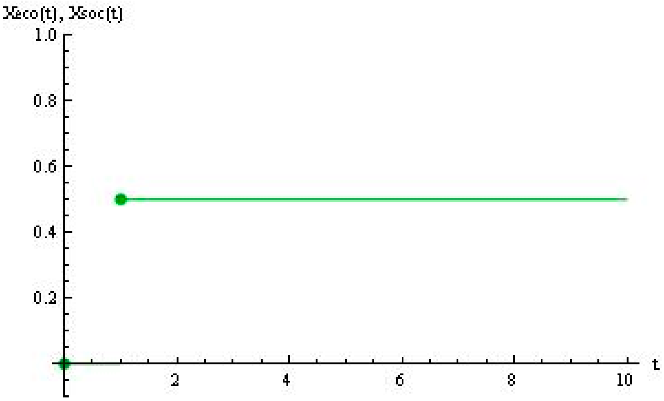
X_eco(t) = X_eco(1) and X_soc(t) = X_soc(1) for each t ≥ 1

(5)

Third, the planning and management time horizon is fixed at T, where environmental and cultural variables achieve their long-run equilibrium. In other words, I focus on external impacts on the natural environment or cultural heritage (e.g., over-exploitation of natural resources or commodification of traditional ceremonies) rather than on external impacts on economic or social features (e.g., cost of living, traffic congestion). Note that alternative contexts would not produce additional insights. For instance, if costs must be borne at each time t to maintain the beneficial effects of both constant (i.e., economic and social) and dynamic (i.e., environmental and cultural) variables, the budget constraint must include a discount rate, where additional savings or investments can only be magnified. Moreover, the stock variable Y(t) can only be positive or 0 (i.e., it can be exhaustible or not). Finally, dynamic data might be required to estimate η_k. For instance, the number of people employed in producing traditional handicrafts at some time after the start of the study period would let us estimate the dynamics of X_cul(t).

Section 2.1, Section 2.2 and Section 2.3 will characterize the three tourism typologies by formalizing them as a single goal within a single framework, whereas Section 2.4 will provide a conceptual reference of the three tourism typologies to be used in subsequent sections. Note that Gossling et al. [14] compared optimisation of many features with maximisation of a single feature; however, they focused only on economic issues. Moreover, tourism goals could be combined by considering impact minimisation together with welfare maximisation or continuity maximisation together with welfare maximisation. See Appendix A for feasible analytical solutions in this context. Finally, Prince and Ioannides [15] suggested management strategies to bridge AT with ST; indeed, tourism goals could be combined by analysing or planning different goals during different periods.

2.1. Responsible Tourism (RT): Minimizing Impacts

The United Nations Educational, Scientific and Cultural Organization (UNESCO) [16] identified the following main (local) features of RT:

• Minimise negative environmental and cultural impacts;
• Enhance the well-being of the host communities;
• Conserve natural and cultural heritage;
• Improve access for physically challenged people.

Mathematically, we choose values of X_env(t) and X_cul(t) in order to:

Min ∑_t=1^T w_env [X_env(t) − X_env(0)]² + w_cul [X_cul(t) − X_cul(0)]²

(6)

where w_env represents the weight of environmental values and w_cul represents the weight of cultural values, s.t.

c_eco [X_eco(t) − X_eco(0)] + c_soc [X_soc(t) − X_soc(0)] + c_env [X_env(t) − X_env(0)] + c_cul [X_cul(t) − X_cul(0)] ≤ Z

X_eco(t) − X_eco(0) ≥ 0, X_soc(t) ≥ X_socrt, Sup X_env ≥ X_env(t) ≥ Inf X_env, Sup X_cul ≥ X_cul(t) ≥ Inf X_cul

where c_eco, c_soc, c_env, and c_cul represent the unitary costs of economic, social, environmental, and cultural investments, respectively; Z represents the budget constraint; X_socrt is the minimum level of social indicators to represent equity concerns; Sup and Inf depict the supremum and the infimum values of the flow variables, respectively; and w_env represents the largest relative weight.

Additional features of RT, such as the need to involve local people in decision-making or to provide meaningful connections between tourists and local people [17] are not formalised and discussed in the rest of my analysis.

Note that carrying capacity (e.g., [18,19]) is a similar concept, but with the emphasis placed upon resources or product life cycles or communities [20]. Moreover, responsible tourism resembles green tourism, social tourism, and volunteer tourism (e.g., [21]). Finally, the following tourism policies could be suggested for responsible tourism: protect land or sea areas [22]; improve relationships with social and regulatory stakeholders, effective management of human resources, market standing, operational efficiency, cost savings, and poverty alleviation [23]; and improve working conditions, promote cultural heritage, and involve local communities [24].

2.2. Sustainable Tourism (ST): Maximizing Welfare

The World Tourism Organization (UNWTO) [25,26] identified the following main (regional) features of ST:

• Meet the economic and social needs of present tourists and their host regions;
• Maintain cultural integrity, essential ecological processes, biological diversity and life-support systems to protect and enhance future opportunities.

Additional features of ST, such as the ability to attain long-run integration of economic, social, and environmental targets [27] are also formalised.

Mathematically, we choose values of X_eco(t), X_soc(t), X_env(t), and X_cul(t) in order to:

Max ∑_t=1^T (1/(1 + ρ)^t) [X_eco(t) − (1/2) p_eco X_eco(t)² + X_soc(t) − (1/2) p_soc X_soc(t)² + X_env(t) − (1/2) p_env X_env(t)² + X_cul(t) − (1/2) p_cul X_cul(t)²]

(7)

where ρ represents the inter-temporal utility discount factor; and p_eco, p_soc, p_env, and p_cul depict the concavity of the quadratic utility function for the economic, social, environmental and cultural items, respectively, s.t.

c_eco [X_eco(t) − X_eco(0)] + c_soc [X_soc(t) − X_soc(0)] + c_env [X_env(t) − X_env(0)] + c_cul [X_cul(t) − X_cul(0)] ≤ Z

X_eco(t) − X_eco(0) ≥ 0, X_soc(t) − X_soc(0) ≥ 0, X_env(t) − X_env(0) ≥ 0, X_cul(t) − X_cul(0) ≥ 0

where X_eco(t) = X_eco(1) and X_soc(t) = X_soc(1) for each t ≥ 1.

Note that sustainable hospitality [11] is a narrower concept, although ST is meaningless unless it is included within the broader context of sustainable development [28]. Moreover, sustainable tourism may include eco-tourism, mountain tourism, indigenous tourism, and rural tourism [29]. Finally, the following tourism policies could be suggested for sustainable tourism: cooperative tools on a project basis, such as dissemination of information by conferences, networking, technical assistance or cooperation, and capacity building by creating awareness and knowledge [1]; voluntary tools on a project basis, such as technical reports on best practices and policy recommendations and project financing [2]; financing tools on a project basis for social responsibility, market competition, quality perception, and technological innovation, such as COM(2003)716 “Basic orientations for the sustainability of European tourism”, COM(2007)621 “Agenda for a sustainable and competitive European tourism”, COM(2010)352 “Europe, the world’s No. 1 tourist destination: a new political framework for tourism in Europe”; and market-based instruments, such as fiscal incentives (e.g., tax relief, grants, matching funding) or benefits in kind [4].

2.3. Alternative Tourism (AT): Maximizing the Continuity

UNWTO [30] identifies the following main (local) features of AT:

• Maintain ancestral cultures;
• Preserve nature;
• Alleviate poverty.

Mathematically, we choose values of X_env(t) and X_cul(t) in order to:

Min ∑_t=1^T w_env [X_env(t) − X_env(T)]² + w_cul [X_cul(t) − X_cul(T)]²

(8)

s.t.

c_eco [X_eco(t) − X_eco(0)] + c_soc [X_soc(t) − X_soc(0)] + c_env [X_env(t) − X_env(0)] + c_cul [X_cul(t) − X_cul(0)] ≤ Z

X_eco(t) − X_eco(0) ≥ 0, X_soc(t) ≥ X_socat, Sup X_env ≥ X_env(t) ≥ Inf X_env, Sup X_cul ≥ X_cul (t) ≥ Inf X_cul

where X_socat is the minimum level of social indicators to represent equity concerns, with w_cul being the largest relative weight. Additional features of AT, such as small-scale and locally controlled decisions or tight interactions between tourists and the host population [15], are not formalised and discussed in the rest of my analysis.

Note that the “three bottom lines” is a similar concept, in which all features must be larger than a given threshold [24]. Moreover, alternative tourism resembles geo-tourism, backpacking tourism, homestay (e.g., [31]), gastronomic tourism (e.g., [32]), cycling charity tourism (e.g., [33]), and reality tourism (e.g., [34]). Finally, the following tourism policies could be suggested for alternative tourism: recovery of ceremonies or craftsmanship, restoration of historical buildings or artistic sites, preservation of natural resources and of ancestral cultures, sharing of tourism revenues and access to resources, and relying on typical product–territory relationships such as olive oil or wine production. Yang et al. [35] provide a framework for an LCA application to identify the long-run equilibrium in carrying capacity; Hernandez and Leon [36] provide a predator–prey model to identify the long-run equilibria in physical infrastructure and natural capital; and Albaladejo and Martinez-Garcia [37] provide an endogenous growth model to identify the long-run equilibrium in carrying capacity.

2.4. A Conceptual Reference

Table 1. A conceptual reference for the main characteristics of the tourism typologies.

	Responsible Tourism	Sustainable Tourism	Alternative Tourism
Goal	Minimize impacts	Maximize welfare	Maximize continuity
Main feature	Environment	Economy	Culture
Perspective	Local and action-oriented	Regional and industry-centred	Local and conservation-oriented
Policies	Protect natural areas, improve working conditions	Fund sustainability projects, subsidize sustainable firms	Recover ceremonies or craftsmanship, restore historical buildings or artistic sites
Forms	Green, social, volunteer	Eco-tourism, rural, mountain, indigenous	Geo-tourism, backpacking, homestay, gastronomic, cycling, charity, reality
Ethics	Aristotle	Bentham	Kant
Focused issues	Sustained economic community development without compromising the existing resources for future generations Distributive justice (e.g., disadvantaged and poor people)	Human welfare (e.g., income and employment) & sustained yield of resources deriving from the governance of populations and ecosystems Structural inequalities (e.g., gender, poverty)	Sustained ecosystem biodiversity of individual species in ecosystems used by humans Procedural justice (e.g., hosts & tourists as actors)
Missed issues	Planning and management Global and long-run landscape Hosts and tourists as actors	Long-run landscape Culture-nature relations with allowed substitutions between capitals Host and tourists as actors	Global landscape Planning and management

summarizes the main characteristics of the three tourism typologies in a single framework based on the main institutional references: all four pillars are assumed to be present in all tourism typologies, although with differences in their relative importance (although the social feature is never the main feature); and all three typologies are assumed to have different goals, with RT and AT having a primarily local perspective, whereas ST has a primarily regional perspective. Note that I have associated the goals, main features, and perspectives with a tourism typology to simplify the discussion of the insights presented in the rest of the paper.

Note that the planning context suggests that we can disregard cross-country differences in the impacts of inbound and outbound tourisms. Qureshi et al. [38] provide an econometric model of these impacts. Moreover, I will estimate the policy impacts by disregarding issues of policy integration. Aall et al. [39] discuss policy integration based on coordination, harmonization, and prioritization as well as based on inclusion, consistency, priorities, and reporting. Finally, the planning context suggests that we can disregard the impacts of sustainability on competitiveness. Pulido-Fernandez et al. [40] provide a cross-country analysis of these impacts.

3. Decision-Making Methodologies and Indicators

In this section, I will discuss assessment methodologies and indicators. For the assessment methodologies, I will focus on MCA (i.e., a decision-making tool for selecting projects, where many objectives and criteria are estimated in percentages and combined by using relative weights), CBA (i.e., a set of rules for the economic evaluation of alternative projects, where the aim is to maximise the social welfare by maximising the net social benefits for a referent group of people), WLCA (i.e., an assessment method for selecting products, where material extraction, construction process, maintenance and operation, and recycling upon life cycle completion are evaluated in terms of possible incompatible criteria and then combined by using relative weights), and MLCA (i.e., an assessment method for selecting products, where material extraction, construction process, maintenance and operation, and recycling upon life cycle completion are evaluated in terms of materials or energy) [12] by considering environmental impact analysis (e.g., [41]) as a simple case of MCA, and cost-effectiveness analysis (e.g., [42]) as a simple case of CBA. Arcese et al. [43] provide a methodological discussion of WLCA applied to tourism, whereas Scheepens et al. [44] provide an empirical validation of MLCA for water tourism based on a cost-efficient value creation method.

Table 2. Summary of strengths and weaknesses of multi-criteria analysis (MCA), cost-benefit analysis (CBA), weighted life-cycle assessment (WLCA), monetary life-cycle assessment (MLCA) with reference to tourism planning and management.

	Strengths	Solvable/Practical Weaknesses	Unsolvable/Theoretical Weaknesses
MCA	Applicable to products and destinations Combination of many features	Qualitative evaluations	Decisions depend on weight assessment and criteria combination methodologies Local and short-run approach
CBA	Reference to competitive general equilibrium Applicable to products and destinations	Distributional issues Risk Indirect impactsLocal and short-run approach Lack of data for quantifying benefits and costs	Attempt to evaluate in monetary terms also intangible features
WLCA	Global and long-run approach Combination of many features Applicable to products	Validation and robustness of results Social issues	Inapplicable to destinations Decisions depend on weight assessment and criteria combination methodologies Lack of referent standards for the evaluation
MLCA	Global and long-run approach Applicable to products	Validation and robustness of results Lack of data for quantifying energy and materials	Inapplicable to destinations Attempt to evaluate everything in energy or material terms Social issues

summarises the main strengths and weaknesses of the four assessment methodologies with reference to tourism planning and management. For the indicators, I will identify suitable indicators by assuming consensus among stakeholders. Mihalic [45], Torres-Delgado and Palomeque [46], Torres-Delgado and Saarinen [47], Iliopoulou-Georgudaki et al. [48], Lee and Hsieh [49], Wang et al. [50], Hashemi and Ghaffary [51], and Onder et al. [52] review this subject.

Note that I will not discuss how to integrate indicators with decision-making [53]. Moreover, I will not discuss the technicalities required to produce the indicators, such as entropy analysis [54], neural networks [55], and factor analysis [56]. Finally, I will not discuss how to scale the indicators ([57,58,59]) or how to weight the indicators ([48,49,50,51]).

I have made three main contextual assumptions. First, I will represent potential conflicts between tourists and their hosts by assuming that the interests of tourists are well represented by X_eco (i.e., the willingness to pay of tourists is totally translated into the economic benefits for their hosts). Alternatively, I could have introduced a maximum threshold for conflicts as perceived by tourists or locals, and objectively estimated that threshold in non-monetary terms (e.g., the percentage of tourists willing to come back; the percentage of locals who support tourism development). Hunt and Stronza [60] describe the estimation of resident attitudes towards tourists. Second, I have assumed that there is no tragedy of the commons. In other words, I will assume a participatory planning context by excluding resources that could be appropriated by certain stakeholders, thereby alienating other stakeholders from the use of those resources. Third, I will represent the potential conflicts (e.g., conflicts over the distribution of tourism revenues) between hosts by modifying X_soc (e.g., increasing the minimum X_soc, thereby reducing inequality in X_soc). Note that I will not discuss how to control institutions (e.g., trust, networks, local control; [61]) or to govern institutions (e.g., community-based vs. lease-operation tourism; [62]).

I have made three main simplifying assumptions. First, I have assumed piece-wise linear dynamics; that is, I have assumed the same η for a given range of t values (i.e., η ≠ 0 for t ≤ some reference t and η = 0 for t > the same reference t). Hereafter, I will use η to represent the dynamics of the environmental or cultural indexes, where it represents the rate of increase in the initial value per year. Smooth (rather than piece-wise) nonlinear dynamics (e.g., X(t) = X(0) × exp[−η t]) would only affect the final T. In other words, I disregard seasonality issues ([63,64,65]).

Second, I will assume a non-stationary random walk (i.e., a = 1 and X(t) = X(0) + η t). If a < 1, this would only affect the final T. In particular, the case of η > 0 depicts a renewable resource, net of its use at time t, or the virtuous reduction of pollution, net of its production at time t, towards the resource’s maximum or long-run stable equilibrium level (i.e., X(T) = max X = X(0) + η T). In contrast, the case of η < 0 depicts a non-renewable resource, net of its use at time t, or the vicious reduction of pollution, net of its production at time t, towards the resource’s minimum or long-run stable equilibrium level (i.e., X(T) = min X = X(0) + η T). The case of η = 0 depicts an economic or social variable that produces a constant benefit for each time t ≥ 1 (e.g., a new hotel ensures a given income and employment levels for each year or other period after it opens). Note that the relevant time horizon for planning is determined by the environmental or cultural effects characterized by the smallest T; this is similar to an analysis of competing carrying capacities [66], although it is based on the dynamics of external variables that affect tourism rather than on the number of tourists.

Third, I will standardize the flow of resources with respect to the maximum level of flows for each dynamic variable (i.e., Sup X_k = 1). In particular, investments could generate economic or social impacts that are constant in time, such as income (X_eco ≤ 1) or employment (X_soc ≤ 1). In addition, investments could generate environmental impacts that vary over time, such as increasing renewable resources or pollution production and decreasing non-renewable resources or waste production (X_env(t) ≤ 1) and cultural impacts that vary over time, such as increasing the social fabric or cultural buildings, or decreasing cultural heritage (X_cul(t) ≤ 1).

Figure 1 depicts the resulting dynamics for environmental and cultural features affected by positive and negative external factors, whereas Figure 2 represents the resulting dynamics for economic and social features.

I made three main simplifying standardizations. First, in ST, I will assume an attitude of risk neutrality towards economic issues; in other words, I will standardize the marginal utility of money to 1 (i.e., 1 − p_eco = 1, so that p_eco = 0). This implies that c_eco = 1 + ρ at equilibrium. Moreover, I assumed that the marginal utility at Sup X_k and Inf X_k is 0 (i.e., 1 − p_k Sup X_k = 0 and 1 − p_k Inf X_k = 0) so that p_k = 1/Sup X_k and p_k = 1/Inf X_k. Finally, in RT and AT, I will focus on solutions for the dynamic environmental and cultural variables, whereas solutions for economic and social variables come from meeting the static economic and social constraints and targets, respectively. In particular, I will not focus on long-run equilibria or on their stability conditions (i.e., X_env or X_cul could be unstable if X_env < Inf X_env or X_cul < Inf X_cul move tourists to other destinations, and if it takes long time to restore both X_env and X_cul), but I will focus on paths towards long-run equilibria from above or from below. Indeed, my purpose is to identify differences in investment decisions based on alternative assessment methodologies: assuming a jump to the long-run equilibria would be meaningless for this purpose. Supplemental Material I summarizes the main simplifying assumptions.

3.1. Multi-Criteria Analysis (MCA) vs. Weighted Life-Cycle Assessment (WLCA) for RT

The dynamic RT solutions with WLCA can be described as follows:

$$\begin{array}{ll}{X}_{\mathrm{env}}=& \#\{2c_{\mathrm{env}}{}^2{p}_{\mathrm{cul}}{p}_{\mathrm{soc}}{w}_{\mathrm{cul}}-2c_{\mathrm{env}}{}^3{p}_{\mathrm{cul}}{p}_{\mathrm{soc}}{w}_{\mathrm{cul}}\\ & +c_{\mathrm{env}}{p}_{\mathrm{env}}{w}_{\mathrm{cul}}[-2c_{\mathrm{soc}}{}^2{p}_{\mathrm{cul}}-2c_{\mathrm{soc}}{p}_{\mathrm{cul}}\left(-1+p_{\mathrm{soc}}{X}_{\mathrm{soc}}\right)\\ & +c_{\mathrm{cul}}{p}_{\mathrm{soc}}\left(2-2c_{\mathrm{cul}}-2p_{\mathrm{cul}}{X}_{\mathrm{cul}}\left(0\right)+{\mathsf{\eta }}_{\mathrm{cul}}T{p}_{\mathrm{cul}}{\mathsf{\theta }}_{\mathrm{cul}}\right)]\\ & +c_{\mathrm{cul}}{}^2{p}_{\mathrm{cul}}{p}_{\mathrm{env}}{p}_{\mathrm{soc}}{w}_{\mathrm{env}}\left(4X_{\mathrm{env}}\left(0\right)-{\mathsf{\eta }}_{\mathrm{env}}T{\mathsf{\theta }}_{\mathrm{env}}\right)\}\end{array}$$

(9)

where,

$$\#=1/\left[2p_{\mathrm{cul}}{p}_{\mathrm{env}}{p}_{\mathrm{soc}}\left(c_{\mathrm{env}}{}^2{w}_{\mathrm{cul}}+c_{\mathrm{cul}}{}^2{w}_{\mathrm{env}}\right)\right]$$

and θ_env = 1 and θ_cul = 1 depict positive and consonant environmental and cultural dynamics, θ_env = −1 and θ_cul = −1 depict negative and consonant environmental and cultural dynamics; and similarly for dissonant dynamics (i.e., dynamics in which θ_env and θ_cul have different signs).

$$\begin{array}{ll}{X}_{\mathrm{cul}}=& \#\{2c_{\mathrm{cul}}{}^2{p}_{\mathrm{env}}{p}_{\mathrm{soc}}{w}_{\mathrm{env}}-2c_{\mathrm{cul}}{}^3{p}_{\mathrm{env}}{p}_{\mathrm{soc}}{w}_{\mathrm{env}}\\ & +c_{\mathrm{env}}{}^2{p}_{\mathrm{cul}}{p}_{\mathrm{env}}{p}_{\mathrm{soc}}{w}_{\mathrm{cul}}\left(2X_{\mathrm{cul}}\left(0\right)-{\mathsf{\eta }}_{\mathrm{cul}}T{\mathsf{\theta }}_{\mathrm{cul}}\right)\\ & +c_{\mathrm{cul}}{p}_{\mathrm{cul}}{w}_{\mathrm{env}}[-2c_{\mathrm{soc}}{}^2{p}_{\mathrm{env}}-2c_{\mathrm{soc}}{p}_{\mathrm{env}}\left(-1+p_{\mathrm{soc}}{X}_{\mathrm{soc}}\right)\\ & +c_{\mathrm{env}}{p}_{\mathrm{soc}}\left(2-2c_{\mathrm{env}}-4p_{\mathrm{env}}{X}_{\mathrm{env}}\left(0\right)+{\mathsf{\eta }}_{\mathrm{env}}T{p}_{\mathrm{env}}{\mathsf{\theta }}_{\mathrm{env}}\right)]\}\end{array}$$

(10)

Next, we can calculate the dynamic RT monetary solutions based on the assumption that c_k = w_k:

$$\begin{array}{ll}{\mathrm{X}}_{\mathrm{env}}=& \S \{-2c_{\mathrm{soc}}{}^2{p}_{\mathrm{cul}}{p}_{\mathrm{env}}-2c_{\mathrm{soc}}{p}_{\mathrm{cul}}{p}_{\mathrm{env}}\left(-1+p_{\mathrm{soc}}{X}_{\mathrm{soc}}\right)\\ & +p_{\mathrm{soc}}[2c_{\mathrm{env}}{p}_{\mathrm{cul}}-2c_{\mathrm{env}}{}^2{p}_{\mathrm{cul}}\\ & +c_{\mathrm{cul}}{p}_{\mathrm{env}}(2-2c_{\mathrm{cul}}\\ & +p_{\mathrm{cul}}(-2X_{\mathrm{cul}}\left(0\right)+4X_{\mathrm{env}}\left(0\right)+{\mathsf{\eta }}_{\mathrm{cul}}T{\mathsf{\theta }}_{\mathrm{cul}}\\ & -{\mathsf{\eta }}_{\mathrm{env}}T{\mathsf{\theta }}_{\mathrm{env}}\left)\right)\left]\right\}\end{array}$$

(11)

where,

$$\S =1/\left[\left(c_{\mathrm{cul}}+c_{\mathrm{env}}\right)p_{\mathrm{cul}}{p}_{\mathrm{env}}{p}_{\mathrm{soc}}\right]$$

and

$$\begin{array}{ll}{X}_{\mathrm{cul}}=& \S \left\{-2c_{\mathrm{soc}}{}^2{p}_{\mathrm{cul}}{p}_{\mathrm{env}}-2c_{\mathrm{soc}}{p}_{\mathrm{cul}}{p}_{\mathrm{env}}\left(-1+p_{\mathrm{soc}}{X}_{\mathrm{soc}}\right)\right\}\\ & +p_{\mathrm{soc}}[-2c_{\mathrm{env}}{}^2{p}_{\mathrm{cul}}-2\left(-1+c_{\mathrm{cul}}\right)c_{\mathrm{cul}}{p}_{\mathrm{env}}\\ & +c_{\mathrm{env}}{p}_{\mathrm{cul}}(2+p_{\mathrm{env}}(2X_{\mathrm{cul}}\left(0\right)-4X_{\mathrm{env}}\left(0\right)-{\mathsf{\eta }}_{\mathrm{cul}}T{\mathsf{\theta }}_{\mathrm{cul}}\\ & +{\mathsf{\eta }}_{\mathrm{env}}T{\mathsf{\theta }}_{\mathrm{env}}\end{array}$$

(12)

In other words, if WLCA is applied, the chosen X_env (i.e., X_env*) increases with respect to X_env(0). That is, a larger initial environmental resource implies a larger investment in the environment:

∂X_env*/∂X_env(0) = 2 c_cul² w_env/(c_env² w_cul + c_cul² w_env)

(13)

X_env* decreases with respect to X_cul(0). That is, with a fixed budget for a given planning period, a larger initial cultural heritage implies a smaller investment in the environment:

∂X_env*/∂X_cul(0) = −c_cul w_env c_env/(c_env² w_cul + c_cul² w_env)

(14)

X_env* decreases with respect to X_socrt. That is, reducing social inequality implies a reduction of environmental investments:

∂X_env*/∂X_socrt = −c_soc w_cul c_env/(c_env² w_cul + c_cul² w_env)

(15)

Similar results are obtained if MLCA is applied, where these partial derivatives become 2 c_cul/(c_cul + c_env), −c_cul/(c_cul + c_env), and −c_soc/(c_cul + c_env), respectively. The same results, with appropriate changes in the variable names, can be obtained for cultural investment decisions.

In particular, RT solutions with WLCA depend on T as follows:

$$\frac{\partial X_{\mathrm{env}}}{\partial T}=\frac{c_{\mathrm{cul}}{c}_{\mathrm{env}}{\mathsf{\eta }}_{\mathrm{cul}}{w}_{\mathrm{cul}}{\mathsf{\theta }}_{\mathrm{cul}}-c_{\mathrm{cul}}{}^2{\mathsf{\eta }}_{\mathrm{env}}{w}_{\mathrm{env}}{\mathsf{\theta }}_{\mathrm{env}}}{2\left(c_{\mathrm{env}}{}^2{w}_{\mathrm{cul}}+c_{\mathrm{cul}}{}^2{w}_{\mathrm{env}}\right)}$$

(16)

and,

$$\frac{\partial X_{\mathrm{cul}}}{\partial T}=\frac{c_{\mathrm{cul}}{c}_{\mathrm{env}}{\mathsf{\eta }}_{\mathrm{env}}{w}_{\mathrm{env}}{\mathsf{\theta }}_{\mathrm{env}}-c_{\mathrm{env}}{}^2{\mathsf{\eta }}_{\mathrm{cul}}{w}_{\mathrm{cul}}{\mathsf{\theta }}_{\mathrm{cul}}}{2\left(c_{\mathrm{env}}{}^2{w}_{\mathrm{cul}}+c_{\mathrm{cul}}{}^2{w}_{\mathrm{env}}\right)}$$

(17)

Thus, T can positively and negatively affect both investment decisions, although with an opposite sign, with the magnitude of the effect depending on the unit costs and relative weights.

Next, RT solutions with MLCA depend on T as follows:

$$\frac{\partial X_{\mathrm{env}}}{\partial T}=\frac{c_{\mathrm{cul}}\left({\mathsf{\eta }}_{\mathrm{cul}}{\mathsf{\theta }}_{\mathrm{cul}}-{\mathsf{\eta }}_{\mathrm{env}}{\mathsf{\theta }}_{\mathrm{env}}\right)}{2\left(c_{\mathrm{env}}+c_{\mathrm{cul}}\right)}$$

(18)

and

$$\frac{\partial X_{\mathrm{cul}}}{\partial T}=\frac{c_{\mathrm{env}}\left({\mathsf{\eta }}_{\mathrm{env}}{\mathsf{\theta }}_{\mathrm{env}}-{\mathsf{\eta }}_{\mathrm{cul}}{\mathsf{\theta }}_{\mathrm{cul}}\right)}{2\left(c_{\mathrm{env}}+c_{\mathrm{cul}}\right)}$$

(19)

Thus, a longer time horizon (T) negatively affects environmental investment decisions if the dynamics are dissonant (i.e., θ_env = 1 and θ_cul = −1) and if the cultural dynamic is smaller than the environmental dynamic (i.e., η_cul < η_env). We obtain similar results for the cultural investment decision X_cul* if we apply the same partial derivatives to it. The right approach for RT is WLCA whenever environmental and cultural dynamics are not negligible.

Many indicators in the literature seem to be suitable for a dynamic assessment of the crucial environmental dimensions of RT [67]. For instance, Navarro Jurado et al. [18] identify aspiration levels, reservation levels, and ranges of some ecological indicators (e.g., beach stability, beach quality, a morphodynamic index, the wealth landscape, built-up areas in the first kilometre of coastal strip, vegetation, fauna) that seem to be close to the X_env, minimum X_env, and maximum X_env–minimum X_env that I applied here. Next, Blancas et al. [68] suggest indicators for the environmental dimension of tourism, for both the assessment (e.g., energy intensity or water consumption attributable to tourism) and management or development of policies (e.g., percentage of the destination’s surface considered to be a protected natural area, number of urban wastewater treatment plants per 1000 inhabitants).

3.2. Cost-Benefit Analysis (CBA) vs. Monetary Life-Cycle Assessment (MLCA) for ST

The dynamic ST solutions can be described as follows, based on my assumption that, for each k, the marginal utility equals the marginal cost (1 − p_k X_k = c_k):

$$X_k=\frac{1-c_k\left(1+\mathsf{\rho }\right)}{p_k}-\frac{T{\mathsf{\theta }}_k{\mathsf{\eta }}_k}{2}\le \frac{1}{p_k}$$

(20)

In words, the chosen X_k (i.e., X_k*) decreases with increases in the inter-temporal utility discount factor ρ (i.e., the discounted value of benefits achieved tomorrow will be smaller than the current costs borne today); X_k* also decreases with increasing T if a positive dynamic applies (i.e., θ_k > 0), and decreases to a larger extent if this dynamic is larger (i.e., larger η_k); X_k* is independent of the initial stock.

Note that solutions for environmental and cultural investments are not correlated with each other. Moreover, the level of X_k* is amended to retain equality between the marginal utility and marginal cost (i.e., (1 − p_k X_k)/(1 + ρ) = c_k) by accounting for its average dynamics (i.e., ±(T/2) η_k). However, if utility depends on the additional amount of X_k (i.e., X_k − X_k(0)), then the chosen X_k* would be X_k + X_k(0). Finally, larger T or η_k (i.e., T η_k p_k > (1 + ρ) c_k) might imply the existence of corner solutions for X_k* (i.e., X_k* = max X_k if θ_k η_k > 0 and X_k* = min X_k if θ_k η_k < 0). The right approach for ST is MLCA whenever environmental and cultural dynamics are not negligible.

Many indicators in the literature seem to be suitable for a static assessment of the crucial economic and social dimensions of ST (e.g., [69,70,71]). Torres-Delgado and Saarinen [47] and Blancas et al. [68] discuss indicators at local and national levels, respectively. McLennan et al. [72], Cottrell et al. [73], Paunovic et al. [74], and Perez et al. [5] discuss indicators based on stakeholder assessments. Tanguay et al. [75] describe the most popular indicators. Mikulic et al. [76], Bhuiyan et al. [77], Romero-Padilla et al. [78], Kunasekaran et al. [79], and Mutana and Mukwada [80] discuss various indices based on indicators.

3.3. MCA vs. WLCA for AT

The dynamic AT solutions with WLCA can be described as follows:

$$\begin{array}{ll}{X}_{\mathrm{env}}=& \#\{2c_{\mathrm{env}}{}^2{p}_{\mathrm{cul}}{p}_{\mathrm{soc}}{w}_{\mathrm{cul}}-2c_{\mathrm{env}}{}^3{p}_{\mathrm{cul}}{p}_{\mathrm{soc}}{w}_{\mathrm{cul}}\\ & +c_{\mathrm{cul}}{}^2{p}_{\mathrm{cul}}{p}_{\mathrm{env}}{p}_{\mathrm{soc}}{w}_{\mathrm{env}}(2X_{\mathrm{env}}\left(T\right)+2X_{\mathrm{env}}\left(0\right)\\ & -{\mathsf{\eta }}_{\mathrm{env}}T{\mathsf{\theta }}_{\mathrm{env}})\\ & +c_{\mathrm{env}}{p}_{\mathrm{env}}{w}_{\mathrm{cul}}[-2c_{\mathrm{soc}}{}^2{p}_{\mathrm{cul}}-2c_{\mathrm{soc}}{p}_{\mathrm{cul}}(-1+p_{\mathrm{soc}}{X}_{\mathrm{soc}})\\ & +c_{\mathrm{cul}}{p}_{\mathrm{soc}}(2-2c_{\mathrm{env}}-2p_{\mathrm{cul}}{X}_{\mathrm{cul}}\left(T\right)-2p_{\mathrm{cul}}{X}_{\mathrm{cul}}\left(0\right)\\ & +{\mathsf{\eta }}_{\mathrm{cul}}T{p}_{\mathrm{cul}}{\mathsf{\theta }}_{\mathrm{cul}}\left)\right]\}\end{array}$$

(21)

where,

$$\#=1/\left[2p_{\mathrm{cul}}{p}_{\mathrm{env}}{p}_{\mathrm{soc}}\left(c_{\mathrm{env}}{}^2{w}_{\mathrm{cul}}+c_{\mathrm{cul}}{}^2{w}_{\mathrm{env}}\right)\right]$$

and

$$\begin{array}{ll}{X}_{\mathrm{cul}}=& \#\{2c_{\mathrm{cul}}{}^2{p}_{\mathrm{env}}{p}_{\mathrm{soc}}{w}_{\mathrm{env}}-2c_{\mathrm{cul}}{}^3{p}_{\mathrm{env}}{p}_{\mathrm{soc}}{w}_{\mathrm{env}}\\ & +c_{\mathrm{env}}{}^2{p}_{\mathrm{cul}}{p}_{\mathrm{env}}{p}_{\mathrm{soc}}{w}_{\mathrm{cul}}(2X_{\mathrm{cul}}\left(T\right)-{\mathsf{\eta }}_{\mathrm{cul}}T{\mathsf{\theta }}_{\mathrm{cul}})\\ & +c_{\mathrm{cul}}{p}_{\mathrm{cul}}{w}_{\mathrm{env}}[-2c_{\mathrm{soc}}{}^2{p}_{\mathrm{env}}-2c_{\mathrm{soc}}{p}_{\mathrm{env}}(-1+p_{\mathrm{soc}}{X}_{\mathrm{soc}})\\ & +c_{\mathrm{env}}{p}_{\mathrm{soc}}(2-2c_{\mathrm{env}}-2p_{\mathrm{env}}{X}_{\mathrm{env}}\left(T\right)-2p_{\mathrm{env}}{X}_{\mathrm{env}}\left(0\right)\\ & +{\mathsf{\eta }}_{\mathrm{env}}T{p}_{\mathrm{env}}{\mathsf{\theta }}_{\mathrm{env}}\left)\right]\}\end{array}$$

(22)

Next, the dynamic AT monetary solutions can be described as follows based on my assumption that c_k = w_k:

$$\begin{array}{ll}{X}_{\mathrm{env}}=& \S \{-2c_{\mathrm{soc}}{}^2{p}_{\mathrm{cul}}{p}_{\mathrm{env}}-2c_{\mathrm{soc}}{p}_{\mathrm{cul}}{p}_{\mathrm{env}}\left(-1+p_{\mathrm{soc}}{X}_{\mathrm{soc}}\right)\\ & +p_{\mathrm{soc}}[2c_{\mathrm{env}}{p}_{\mathrm{cul}}-2c_{\mathrm{env}}{}^2{p}_{\mathrm{cul}}\\ & +c_{\mathrm{cul}}{p}_{\mathrm{env}}(2-2c_{\mathrm{cul}}\\ & +p_{\mathrm{cul}}(-2X_{\mathrm{cul}}\left(T\right)+2X_{\mathrm{env}}\left(T\right)+2X_{\mathrm{env}}\left(0\right)+{\mathsf{\eta }}_{\mathrm{cul}}T{\mathsf{\theta }}_{\mathrm{cul}}\\ & -{\mathsf{\eta }}_{\mathrm{env}}T{\mathsf{\theta }}_{\mathrm{env}}\left)\right)\left]\right\}\end{array}$$

(23)

where,

$$\S =1/\left[\left(c_{\mathrm{cul}}+c_{\mathrm{env}}\right)p_{\mathrm{cul}}{p}_{\mathrm{env}}{p}_{\mathrm{soc}}\right]$$

and

$$\begin{array}{ll}{X}_{\mathrm{cul}}=& \S \{-2c_{\mathrm{soc}}{}^2{p}_{\mathrm{cul}}{p}_{\mathrm{env}}-2c_{\mathrm{soc}}{p}_{\mathrm{cul}}{p}_{\mathrm{env}}\left(-1+p_{\mathrm{soc}}{X}_{\mathrm{soc}}\right)\\ & +p_{\mathrm{soc}}[-2c_{\mathrm{env}}{}^2{p}_{\mathrm{cul}}-2\left(-1+c_{\mathrm{cul}}\right)c_{\mathrm{cul}}{p}_{\mathrm{env}}+c_{\mathrm{env}}{p}_{\mathrm{cul}}(2\\ & +p_{\mathrm{env}}(2X_{\mathrm{cul}}\left(T\right)-2X_{\mathrm{env}}(T)-2X_{\mathrm{env}}\left(0\right)-{\mathsf{\eta }}_{\mathrm{cul}}T{\mathsf{\theta }}_{\mathrm{cul}}\\ & +{\mathsf{\eta }}_{\mathrm{env}}T{\mathsf{\theta }}_{\mathrm{env}}\left)\right)\left]\right\}\end{array}$$

(24)

In other words, if WLCA is applied, the chosen X_env (i.e., X_env*) increases with respect to X_env(0). That is, a larger initial amount of environmental resources implies a larger investment in the environment:

∂X_env*/∂X_env(0) = c_cul² w_env/(c_env² w_cul + c_cul² w_env)

(25)

X_env* increases with respect to X_env(T). That is, a larger long-run amount of environmental resources implies a larger investment in the environment:

∂X_env*/∂X_env(T) = c_cul² w_env/(c_env² w_cul + c_cul² w_env)

(26)

X_env* does not depend on X_cul(0). That is, a larger initial cultural heritage does not affect investment in the environment (∂X_env*/∂X_cul(0) = 0), and X_env* decreases with respect to X_soc. That is, in the context of a fixed budget for a given planning period, reducing social inequality implies a reduction of environmental investments:

∂X_env*/∂X_soc = −c_soc w_cul c_env/(c_env² w_cul + c_cul² w_env)

(27)

Similar results are obtained if MLCA is applied, where these partial derivatives become c_cul/(c_cul + c_env), 0, and −c_soc/(c_cul + c_env), respectively. We obtain similar results for the cultural investment decision X_cul* if we apply analogous partial derivatives to it.

In particular, AT solutions with WLCA will depend on T as follows:

$$\frac{\partial X_{\mathrm{env}} }{\partial T}=\frac{c_{\mathrm{cul}}{c}_{\mathrm{env}}{\mathsf{\eta }}_{\mathrm{cul}}{w}_{\mathrm{cul}}{\mathsf{\theta }}_{\mathrm{cul}}-c_{\mathrm{cul}}{}^2{\mathsf{\eta }}_{\mathrm{env}}{w}_{\mathrm{env}}{\mathsf{\theta }}_{\mathrm{env}}}{2\left(c_{\mathrm{env}}{}^2{w}_{\mathrm{cul}}+c_{\mathrm{cul}}{}^2{w}_{\mathrm{env}}\right)}$$

(28)

and

$$\frac{\partial X_{\mathrm{cul}}}{\partial T}=\frac{c_{\mathrm{cul}}{c}_{\mathrm{env}}{\mathsf{\eta }}_{\mathrm{env}}{w}_{\mathrm{env}}{\mathsf{\theta }}_{\mathrm{env}}-c_{\mathrm{env}}{}^2{\mathsf{\eta }}_{\mathrm{cul}}{w}_{\mathrm{cul}}{\mathsf{\theta }}_{\mathrm{cul}}}{2\left(c_{\mathrm{env}}{}^2{w}_{\mathrm{cul}}+c_{\mathrm{cul}}{}^2{w}_{\mathrm{env}}\right)}$$

(29)

Next, AT solutions with MLCA will depend on T as follows:

$$\frac{\partial X_{\mathrm{env}}}{\partial T}=\frac{c_{\mathrm{cul}}\left({\mathsf{\eta }}_{\mathrm{cul}}{\mathsf{\theta }}_{\mathrm{cul}}-{\mathsf{\eta }}_{\mathrm{env}}{\mathsf{\theta }}_{\mathrm{env}}\right)}{2\left(c_{\mathrm{env}}+c_{\mathrm{cul}}\right)}$$

(30)

and

$$\frac{\partial X_{cul}}{\partial T}=\frac{c_{\mathrm{env}}\left({\mathsf{\eta }}_{\mathrm{env}}{\mathsf{\theta }}_{\mathrm{env}}-{\mathsf{\eta }}_{\mathrm{cul}}{\mathsf{\theta }}_{\mathrm{cul}}\right)}{2\left(c_{\mathrm{env}}+c_{\mathrm{cul}}\right)}$$

(31)

Thus, a longer time horizon (T) has the same impact on AT and RT investment solutions. Moreover, the impact of the initial amount of environmental resources on investment decisions is larger in RT than in AT. Finally, social targets have the same impacts on AT and RT investment solutions. The right approach for AT is WLCA whenever environmental and cultural dynamics are not negligible.

Few indicators in the literature seem to be suitable for a dynamic assessment of the crucial cultural dimensions of AT [67]. In particular, Blancas et al. [81] suggest indicators for managing the cultural dimension of tourism (e.g., number of cultural properties, practices and expressions inscribed in the UNESCO World Intangible Heritage List or in its Tentative List). Next, Torres-Delgado and Saarinen [47] suggest indicators for assessing the cultural dimension of tourism (e.g., type and amount of training given to tourism employees, employment in producing traditional handicrafts).

4. Comparisons

4.1. Investment Errors with Static Instead of Dynamic Assessments

Comparisons of investment decisions based on static vs. dynamic assessments can be performed theoretically. However, I applied three main standardizations. First, for MLCA, I assumed that ρ = 0 to allow a comparison of ST with RT and AT. Actually, ρ = 0 is the only consistent assumption for an inter-temporal assessment of sustainability for large T. This implies that c_eco = 1 + ρ = 1 at equilibrium. Second, I disregarded the relationships between the environmental and cultural flows and the tourist flows by assuming linear relationships between the former flows and the latter flows and by focusing on the dynamics of the former flows. Third, for MLCA, I equalized the relative weights to the marginal utilities (i.e., 1 − p_k = w_k). This implies that c_k = w_k at equilibrium.

Note that η_env is larger if we consider global instead of local sustainability conditions (e.g., inter-continental flights to a locally sustainable atoll). Moreover, in ST, the explicit value of resources comes from their marginal utility, whereas in RT and AT, the implicit value arises from the distance with respect to the current level in RT and with respect to the long-run equilibrium in AT. Finally, comparisons are feasible, since minimising a quadratic distance function amounts to maximising a quadratic utility function if an implicit negative welfare is attached to gaps between the observed level and the desired level, which can be either the current level or the long-run equilibrium level.

Table 3. Summary of comparisons between wrong static (i.e., MCA and CBA) versus right dynamic (i.e., WLCA and MLCA) solutions. RT = responsible tourism; ST = sustainable tourism, AT = alternative tourism.

	RT	ST	AT
WLCA-MCA	$X_{\mathrm{env}}^{*}\left(WLCA\right)-X_{\mathrm{env}}^{*}\left(MCA\right)=\frac{c_{\mathrm{cul}}T\left(c_{\mathrm{env}}{\mathsf{\theta }}_{\mathrm{cul}}{\mathsf{\eta }}_{\mathrm{cul}}{w}_{\mathrm{cul}}-c_{\mathrm{cul}}{\mathsf{\theta }}_{\mathrm{env}}{\mathsf{\eta }}_{\mathrm{env}}{w}_{\mathrm{env}}\right)}{2\left(c_{\mathrm{env}}{}^2{w}_{\mathrm{cul}}+c_{\mathrm{cul}}{}^2{w}_{\mathrm{env}}\right)}$ $X_{\mathrm{cul}}^{*}\left(WLCA\right)-X_{\mathrm{cul}}^{*}\left(MCA\right)=\frac{c_{\mathrm{env}}T\left(c_{\mathrm{cul}}{\mathsf{\theta }}_{\mathrm{env}}{\mathsf{\eta }}_{\mathrm{env}}{w}_{\mathrm{env}}-c_{\mathrm{env}}{\mathsf{\theta }}_{\mathrm{cul}}{\mathsf{\eta }}_{\mathrm{cul}}{w}_{\mathrm{cul}}\right)}{2\left(c_{\mathrm{env}}{}^2{w}_{\mathrm{cul}}+c_{\mathrm{cul}}{}^2{w}_{\mathrm{env}}\right)}$ $X_k^{*}\left(WLCA\right)-X_k^{*}\left(MCA\right)$ if $c_{\mathrm{cul}}{\mathsf{\theta }}_{\mathrm{env}}{\mathsf{\eta }}_{\mathrm{env}}{w}_{\mathrm{env}}=c_{\mathrm{env}}{\mathsf{\theta }}_{\mathrm{cul}}{\mathsf{\eta }}_{\mathrm{cul}}{w}_{\mathrm{cul}}$		$X_{\mathrm{env}}^{*}\left(WLCA\right)-X_{\mathrm{env}}^{*}\left(MCA\right)=\frac{c_{\mathrm{cul}}T\left(c_{\mathrm{env}}{\mathsf{\theta }}_{\mathrm{cul}}{\mathsf{\eta }}_{\mathrm{cul}}{w}_{\mathrm{cul}}-c_{\mathrm{cul}}{\mathsf{\theta }}_{\mathrm{env}}{\mathsf{\eta }}_{\mathrm{env}}{w}_{\mathrm{env}}\right)}{2\left(c_{\mathrm{env}}{}^2{w}_{\mathrm{cul}}+c_{\mathrm{cul}}{}^2{w}_{\mathrm{env}}\right)}$ $X_{\mathrm{cul}}^{*}\left(WLCA\right)-X_{\mathrm{cul}}^{*}\left(MCA\right)=\frac{c_{\mathrm{env}}T\left(c_{\mathrm{cul}}{\mathsf{\theta }}_{\mathrm{env}}{\mathsf{\eta }}_{\mathrm{env}}{w}_{\mathrm{env}}-c_{\mathrm{env}}{\mathsf{\theta }}_{\mathrm{cul}}{\mathsf{\eta }}_{\mathrm{cul}}{w}_{\mathrm{cul}}\right)}{2\left(c_{\mathrm{env}}{}^2{w}_{\mathrm{cul}}+c_{\mathrm{cul}}{}^2{w}_{\mathrm{env}}\right)}$ $X_k^{*}\left(WLCA\right)-X_k^{*}\left(MCA\right)$ if $c_{\mathrm{cul}}{\mathsf{\theta }}_{\mathrm{env}}{\mathsf{\eta }}_{\mathrm{env}}{w}_{\mathrm{env}}=c_{\mathrm{env}}{\mathsf{\theta }}_{\mathrm{cul}}{\mathsf{\eta }}_{\mathrm{cul}}{w}_{\mathrm{cul}}$
MLCA-CBA		$X_k^{*}\left(MLCA\right)-X_k^{*}\left(CBA\right)=\frac{T{\mathsf{\theta }}_k{\mathsf{\eta }}_k}{2}$
MLCA-MCA	$X_{\mathrm{env}}^{*}\left(MLCA\right)-X_{\mathrm{env}}^{*}\left(MCA\right)=\frac{c_{\mathrm{cul}}\left({\mathsf{\theta }}_{\mathrm{cul}}{\mathsf{\eta }}_{\mathrm{cul}}-{\mathsf{\theta }}_{\mathrm{env}}{\mathsf{\eta }}_{\mathrm{env}}\right)T}{2\left(c_{\mathrm{cul}}+c_{\mathrm{env}}\right)}$ $X_{\mathrm{cul}}^{*}\left(MLCA\right)-X_{\mathrm{cul}}^{*}\left(MCA\right)=\frac{c_{\mathrm{env}}\left({\mathsf{\theta }}_{\mathrm{env}}{\mathsf{\eta }}_{\mathrm{env}}-{\mathsf{\theta }}_{\mathrm{cul}}{\mathsf{\eta }}_{\mathrm{cul}}\right)T}{2\left(c_{\mathrm{cul}}+c_{\mathrm{env}}\right)}$ $X_k^{*}\left(MLCA\right)-X_k^{*}\left(MCA\right)$ if ${\mathsf{\theta }}_{\mathrm{env}}{\mathsf{\eta }}_{\mathrm{env}}={\mathsf{\theta }}_{\mathrm{cul}}{\mathsf{\eta }}_{\mathrm{cul}}$		$X_{\mathrm{env}}^{*}\left(MLCA\right)-X_{\mathrm{env}}^{*}\left(MCA\right)=\frac{c_{\mathrm{cul}}\left({\mathsf{\theta }}_{\mathrm{cul}}{\mathsf{\eta }}_{\mathrm{cul}}-{\mathsf{\theta }}_{\mathrm{env}}{\mathsf{\eta }}_{\mathrm{env}}\right)T}{2\left(c_{\mathrm{cul}}+c_{\mathrm{env}}\right)}$ $X_{\mathrm{cul}}^{*}\left(MLCA\right)-X_{\mathrm{cul}}^{*}\left(MCA\right)=\frac{c_{\mathrm{env}}\left({\mathsf{\theta }}_{\mathrm{env}}{\mathsf{\eta }}_{\mathrm{env}}-{\mathsf{\theta }}_{\mathrm{cul}}{\mathsf{\eta }}_{\mathrm{cul}}\right)T}{2\left(c_{\mathrm{cul}}+c_{\mathrm{env}}\right)}$ $X_k^{*}\left(MLCA\right)-X_k^{*}\left(MCA\right)$ if ${\mathsf{\theta }}_{\mathrm{env}}{\mathsf{\eta }}_{\mathrm{env}}={\mathsf{\theta }}_{\mathrm{cul}}{\mathsf{\eta }}_{\mathrm{cul}}$

summarises the errors if a wrong static methodology (i.e., MCA and CBA) instead of a right dynamic methodology (i.e., WLCA and MLCA) is applied.

In words, if w_env > w_cul in RT and w_env < w_cul in AT, the couples of η_env and η_cul such that there is excessive environmental investment (i.e., an error level) if MCA is applied instead of WLCA are smaller in RT than in AT. If negative and consonant environmental and cultural dynamics apply, ST shows the smallest error level. In contrast, if MLCA is applied so that the weights equal the marginal costs, there is no difference between RT and AT in terms of error level. Moreover, if MLCA is applied to ST, the errors are not correlated (i.e., cross-dependence on environmental and cultural dynamics), whereas errors of environmental or cultural investments are correlated if WLCA is applied to RT and AT, with errors for AT more correlated than for RT. In contrast, if MLCA is applied, there is no difference between RT and AT in terms of error correlation. Finally, dependence on the couples of tentatively estimated η_env and η_cul (i.e., error likelihood) if MCA is applied instead of WLCA is smaller in AT than in RT. If negative and consonant environmental and cultural dynamics apply, ST shows the smallest error likelihood. In contrast, if MLCA is applied, there is no difference between RT and AT in terms of error likelihood.

In summary, if negative and consonant environmental and cultural dynamics apply, the overall ranking if a wrong static instead of a right dynamic approach is adopted (e.g., due to a lack of data) is ST > RT > AT if MCA and CBA are applied instead of WLCA and MLCA, respectively; the overall ranking is ST > RT = AT if MCA and CBA are applied instead of MLCA.

Note that errors in RT and AT are never 0 if the dynamics have opposite signs. Moreover, errors do not depend on X_soc in RT and AT, although investments depend on X_soc, where it is likely that X_soc in RT < X_soc in AT, with either the same or different distributions. Finally, investments depend on X_k(0) in RT and on X_k(T) in AT, but the errors do not. In summary, unless marginal benefits equal marginal costs, potential interactions between X_env and X_cul are reflected in the budget constraint, since accounting for the dynamics of external factors could save money that could to be used to improve other beneficial effects or to reduce other detrimental effects.

4.2. Investment Differences with WLCA Instead of MLCA

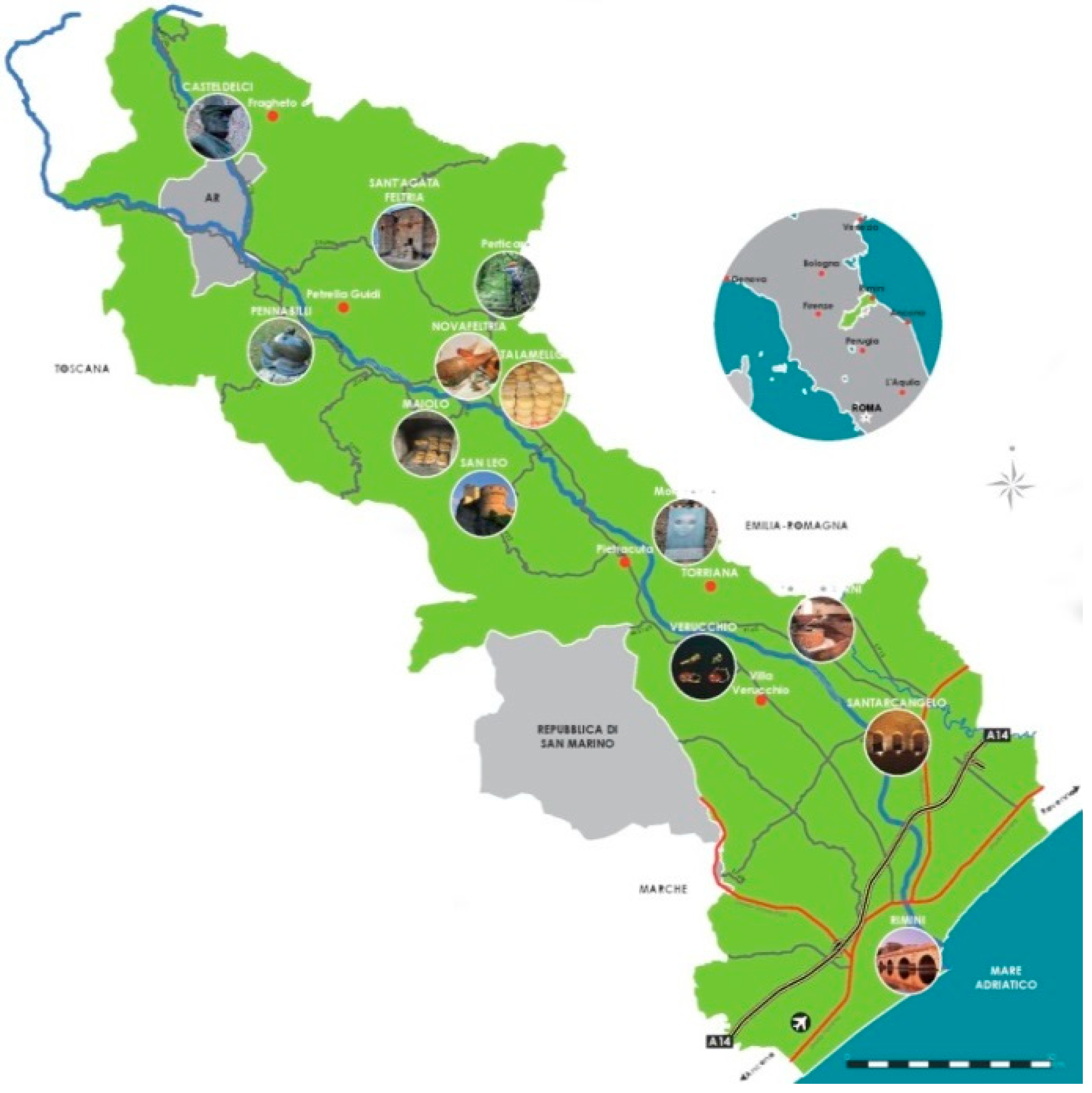
Comparisons of investment decisions based on WLCA vs. MLCA must be performed empirically. Therefore, I will refer to a case study of the Alta Val Marecchia planning area, located in Northern Italy’s Rimini Province, within the Emilia-Romagna region (Figure 3). Note that I did not choose this case study because of its unique characteristics (i.e., I could have chosen many other areas with similar features), but rather because of data availability (i.e., I could have chosen any area with similar data). The study region consists of seven municipalities: Casteldelci, Maiolo, Novafeltria, Pennabilli, San Leo, Sant’Agata, and Talamello.

This area is an interesting case study for two main reasons. First, it is a good example of an area where tourism depends on both natural and cultural resources; tourism firms accounted for 6.9% of the total number of companies in 2011 [82], and 7.7% of these firms were hotels or restaurants. In addition, there is a natural park (i.e., Sasso Simone and Simoncello, 4847 ha), and there are four ancient castles in San Leo, Sant’Agata, Pennabilli, and Casteldelci.

Second, the seven municipalities were added to Rimini Province in 2009, so a large budget (i.e., 12 million euros) was allocated by the Emilia-Romagna Region from 2010 to 2013, with the following distribution: 22% to improve competitiveness, 18% to improve urban quality and sustainable transportation (e.g., private transportation to be replaced by public, trucks to be replaced by trains), 16% to improve the environment, and 44% to improve culture and other local potential [83]. I will use these percentages to calculate costs (i.e., c_eco, c_soc, c_env, and c_cul) by disregarding the small amounts of funds (i.e., 10,000 to 20,000 euros each) for specified projects chosen annually by the Emilia-Romagna Region. In contrast, I will refer to the priorities stated by local firms (i.e., 33% for incentives to firms; 51% for infrastructure including roads, hospitals and schools; 6% for the environment, including a dam for hydropower; and 4% for culture; [84]) to calculate the relative weights (i.e., w_eco, w_soc, w_env, and w_cul). Note that these percentages do not sum up to 100, since 6% of local firms did not specify a priority.

For tourism structures, there are 11 hotels (i.e., one in San Leo, two in Sant’Agata, three in Pennabilli, one in Casteldelci, four in Novafeltria), and 63 alternatives to hotels (40% bed and breakfast (B&Bs), 30% agritourist locations, and 30% camping).

The tourism flows are point sources. Indeed, in San Leo, 74,390 castle tickets were sold in 2016. Moreover, the available time series refers to all of the tourist presence in Rimini Province, although agritourist firms are most typical of this area. Finally, single municipality reports record around 50,000 people per year visiting Pennabilli for fairs, street artist festivals, and antique markets; around 150,000 people per year visited Sant’Agata for Christmas, truffle fairs, and novel festivals; and around 50,000 people per year visited San Leo for fairs and music festivals.

Therefore, I will normalize per capita expenditures for economic and social issues by dividing the expenditures by the number of residents (i.e., 17,374 inhabitants in 2016). Moreover, I will normalize per capita expenditures for environmental issues based on stays at hotel alternatives (i.e., 50,079 in 2016). Finally, I will normalize per capita expenditures for cultural issues based on stays in hotels (i.e., 50,840 in 2016; [85]). This leads to Emilia-Romagna Region expenditures of 51 and 41 euro per inhabitant per year for economic and social issues, and of 13 and 35 euros per tourist per year for environmental and cultural issues. Note that stays with agritourist firms reached a peak in 2014 (i.e., 19 521), the year after the planning period of 2010 to 2013.

For the tourism sector, the occupancy rate of accommodations was 15% [86]. Thus, I will fix X_env(0) = 50,079 and X_cul(0) = 50,840 based on the observed data in 2016, and set the carrying capacity at twice these values (i.e., Sup X_env = 2 × 50,079, Sup X_cul = 2 × 50,840) because doubling the occupancy rate seems to be a plausible target to achieve.

For the area’s economy, the value added per inhabitant was 24 900 euros, the participation in the tourism industry for residents aged 15 to 64 years is 62.9%, the unemployment rate is 9.1%, and the value added per employee is 58,500 euros. Thus, I estimated X_soc in AT by assuming that the objective was to eliminate unemployment (i.e., 994 people) so that 9.1% of the residents would receive employment benefits, and I estimated X_soc in RT by assuming that the target was to eliminate unemployment (i.e., 994 people) so that the average value added would increase by 6.1%, under the assumption of a uniform distribution.

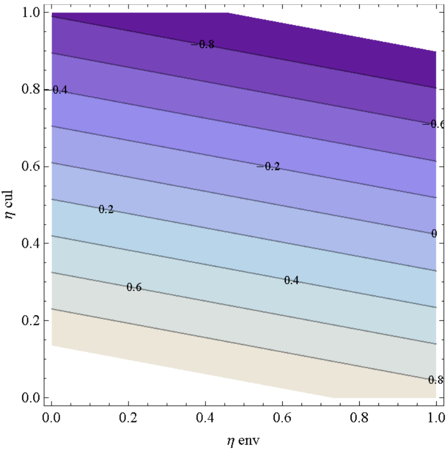
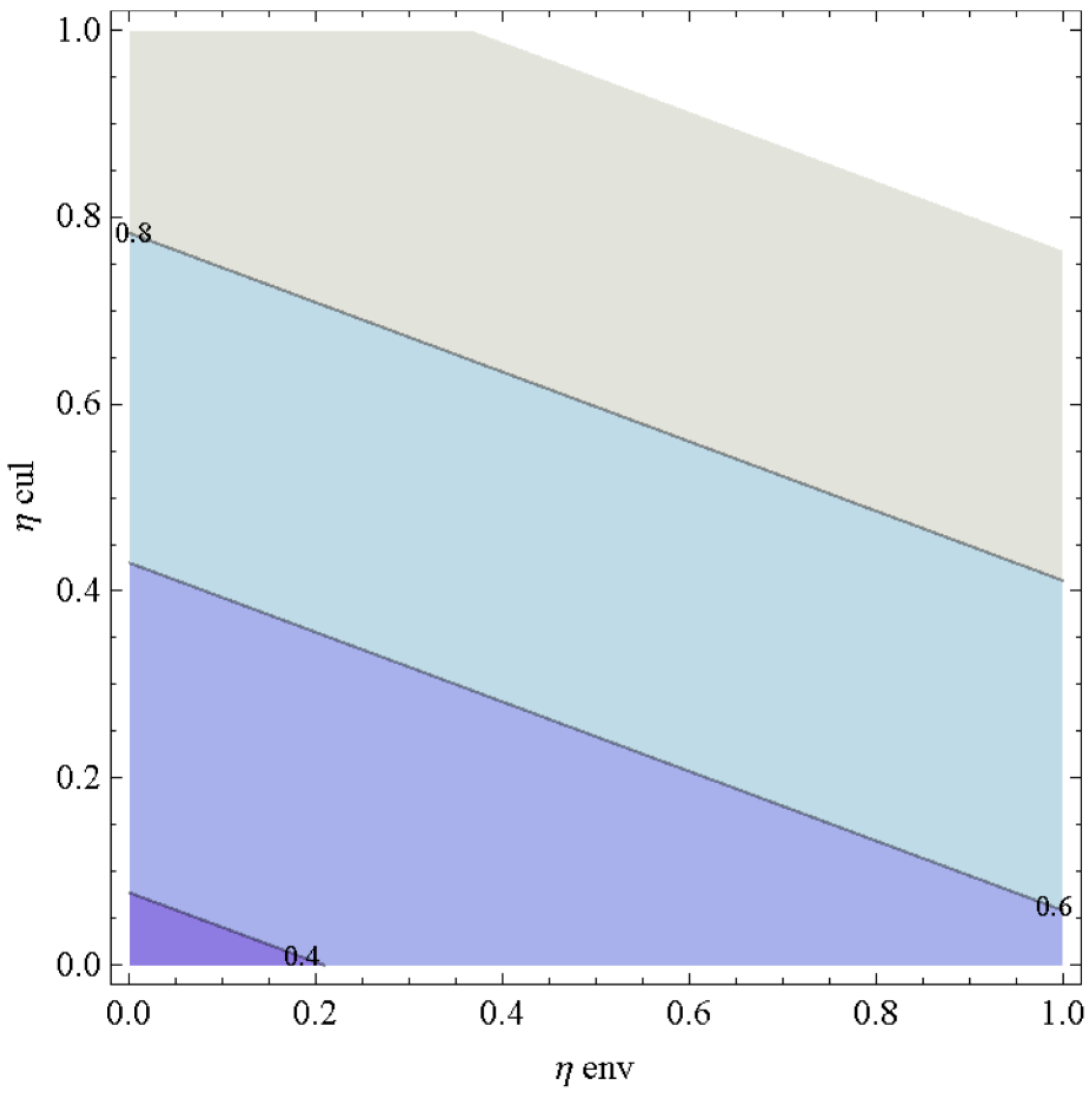
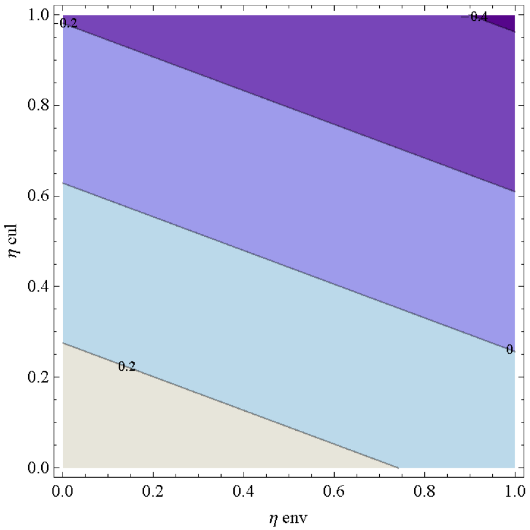
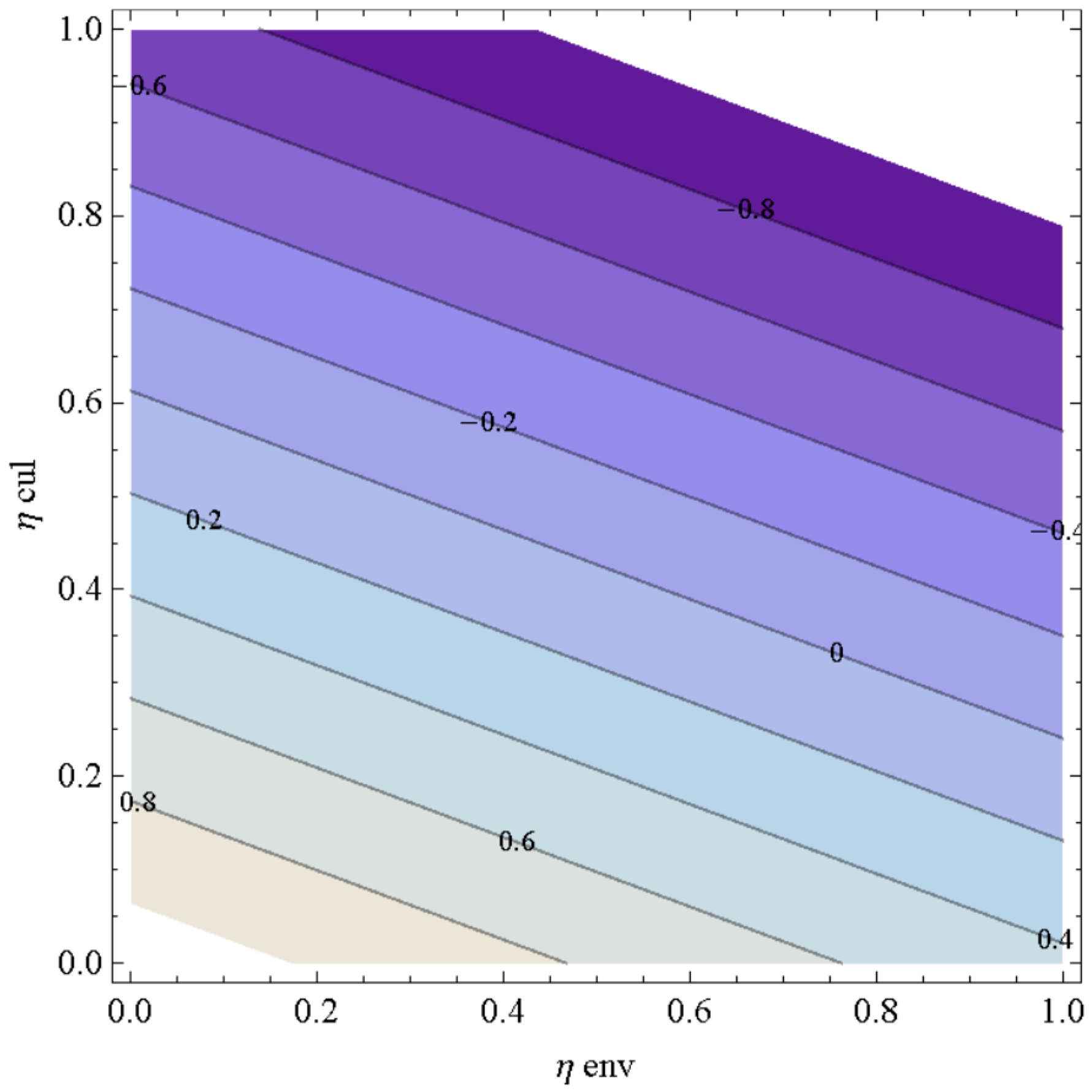
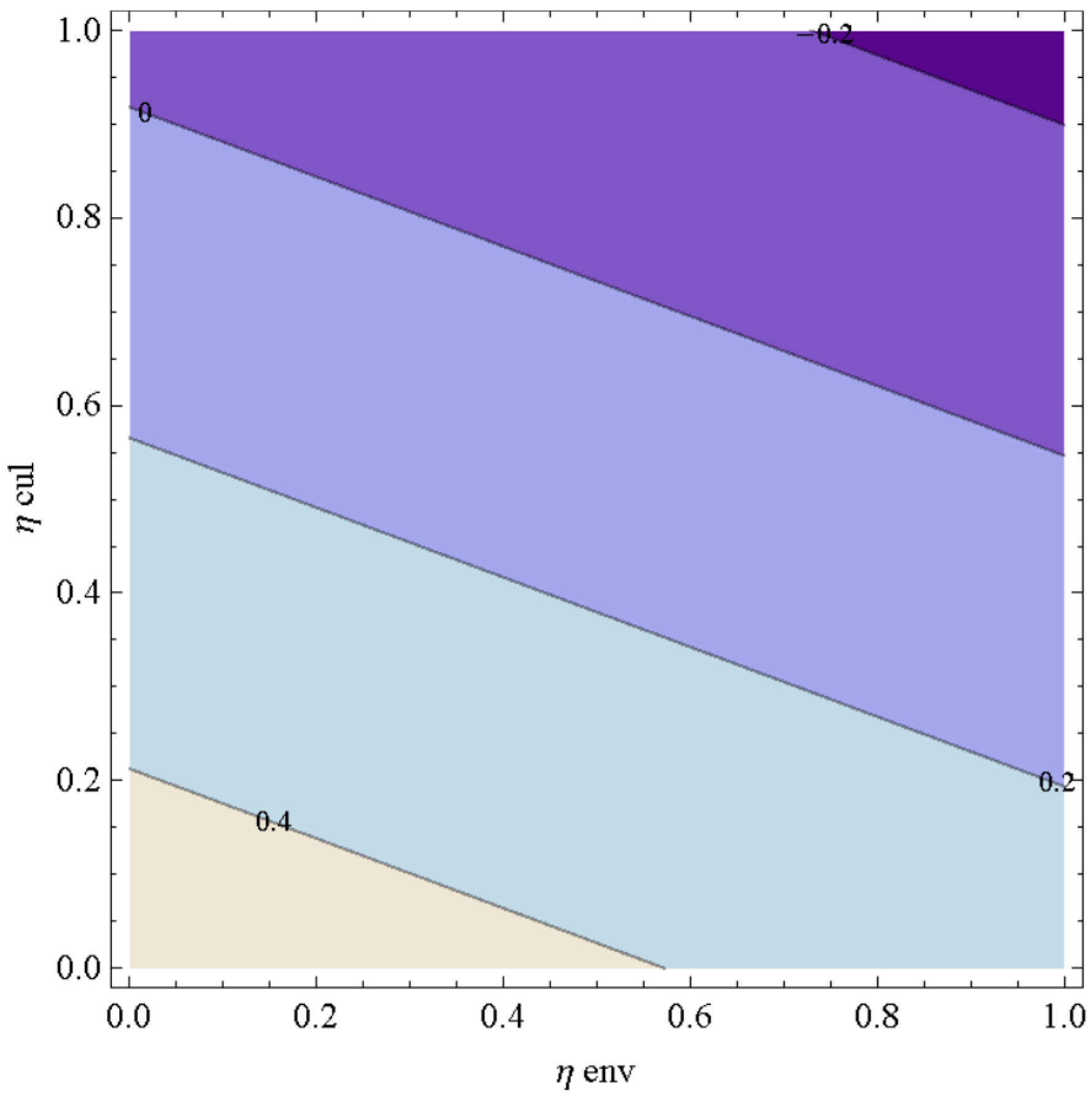
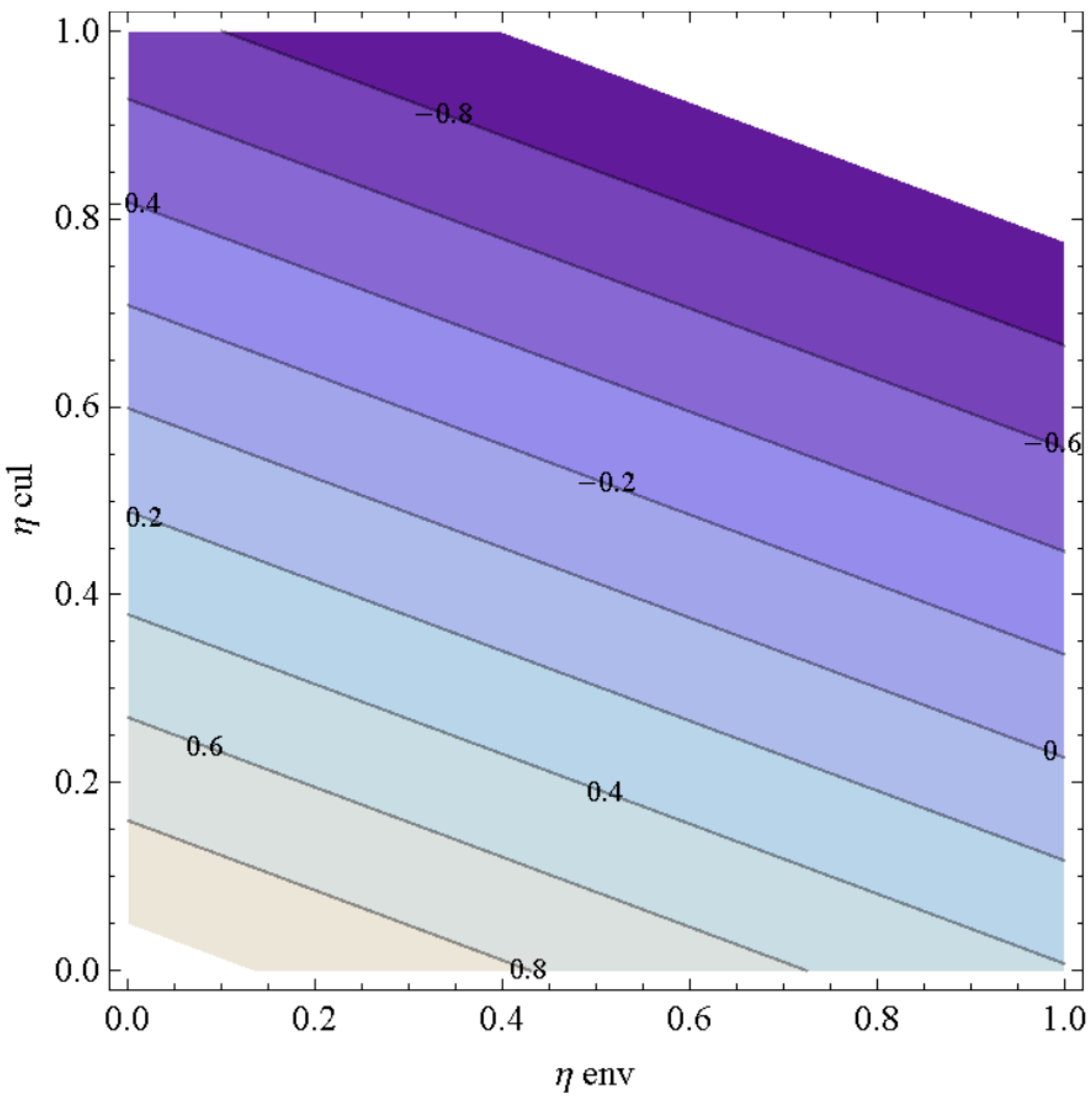
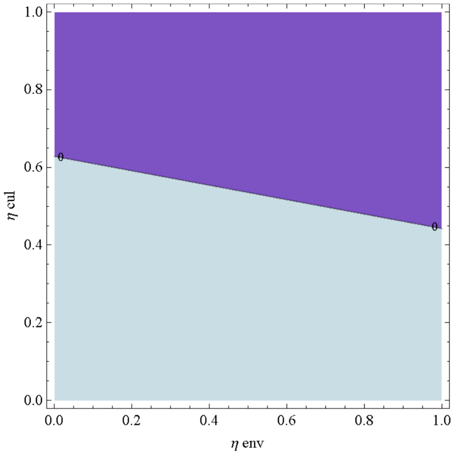
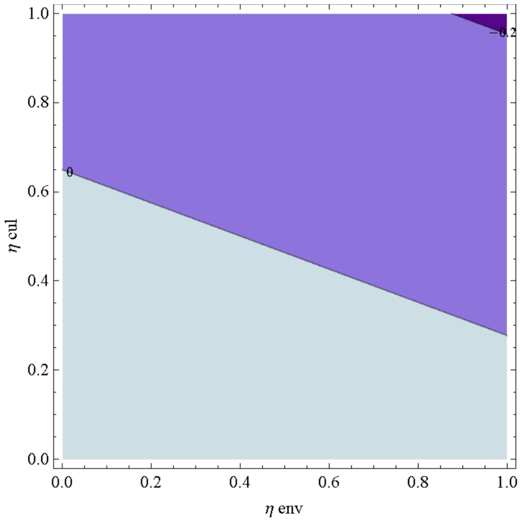
Figure 4 and Figure 5 compare the environmental investment decisions (X_env) in RT vs. ST, with these values estimated using WLCA and MLCA, respectively. Figure 6 and Figure 7 compare X_env in AT vs. ST, with these values estimated by WLCA and MLCA, respectively. Note that the slope of the level curves is −0.37 for all these figures (i.e., differences in investments are equally correlated with the values of cultural dynamics). Supplemental Material II summarizes the relationships among figures, which depend on different assumptions.

Note that I assumed that η measures the dynamics of external factors for a 5-year period, by fixing T at 5 because 25-year planning horizons (i.e., five 5-year periods) seem to be reasonable for the region’s natural environmental and cultural heritage. Moreover, I assumed that p_soc = 1 so that the marginal utility would be positive whenever social investments affected a fraction of or the whole resident population, with the population normalized to 1 (i.e., X_soc ≤ 1). Finally, I normalised X_env(0) and X_cul(0) to 0.5, Sup X_env and Sup X_cul to 1, and the long-run X_env(T) and X_cul(T) to 0.75, with the objective of accounting for the aforementioned potential doubling of the current occupancy rate. This implies that investment differences are in the range [–1, 1].

The values of the level curves in Figure 4 suggest that when RT is properly assessed (with WLCA), this tourism typology is more precautionary (i.e., resource preservation is more likely) than when ST is correctly assessed (with MLCA) with plausible environmental and cultural dynamics (i.e., η_env < 0.5 and η_cul < 0.5; in words, this represents a decay rate smaller than 50% over the 5 years). Comparing the distance between the level curves in Figure 5 and Figure 4 suggests that applying monetary or single-unit measurements (i.e., MLCA) to RT is riskier (i.e., differences in investments based on different methodologies are more sensitive to environmental and cultural dynamics).

The values of the level curves in Figure 6 and Figure 4 suggest that AT is more precautionary than RT at all levels of environmental and cultural dynamics (i.e., at the same environmental and cultural dynamics, a larger investment is chosen; e.g., at η_env = η_cul = 0.1, X_env* = 0.27 in RT and X_env* = 0.44 in AT). Note that both differences in environmental investments (i.e., RT − ST and AT − ST) are −0.18 + 0.25 η_cul, which is positive for sufficiently large values of η_cul (i.e., RT and AT are less risky than ST). Comparing the distance between the level curves in Figure 7 and Figure 5 suggests that applying monetary or single-unit measurements (i.e., MLCA) to AT is as risky as when they are applied to RT (e.g., at η_env = η_cul = 0.1, X_env* = 0.86 in RT and X_env* = 0.84 in AT).

Figure 8 illustrates the effects of policies implemented in the form of cost subsidies, where c_env is divided by 2 because a subsidisation around 50% has been applied in Italy to support the use of renewable energy. See Figure A1 in Appendix B for RT assessed by MLCA. Comparing the values and slopes of the level curves in Figure 8 and Figure 4 suggests that subsidizing the environmental costs makes environmental decisions based on RT properly assessed (i.e., using WLCA) similar to the decisions based on ST properly assessed (i.e., using MLCA); that is, RT − ST is 0 or close to 0 for a large set of environmental and cultural dynamics, and RT − ST is uncorrelated with the value of cultural dynamics (i.e., the level curves are flatter) to a larger extent.

Figure 9 shows the results if policies are expressed as environmental concerns, with w_env multiplied by 2 because doubling its current value seems to be a plausible target to achieve for the study area. See Figure A2 in Appendix B for RT assessed by MLCA. Comparing the values of the level curves in Figure 9 and Figure 4 suggests that an information campaign to increase stakeholder concern for the environment would make the environmental decisions based on RT properly assessed (with WLCA) similar to the decisions based on ST properly assessed (with MLCA). That is, RT − ST is 0 or close to 0 for a large set of values of environmental and cultural dynamics. Comparing the values and slopes of the level curves in Figure 9 and Figure 8 suggests that subsidizing environmental costs would have effects similar to those of an information campaign for increasing stakeholder concerns for the environment, although at a smaller set of values for cultural dynamics.

Note that using relative budgets as relative weights leads to the same investment decisions obtained by applying monetary assessments (i.e., investment decisions depend on the difference between politician and stakeholder priorities). Moreover, standardisations per inhabitant and per tourist (i.e., 51, 41, 13, and 35 euros per person for economic, social, environmental, and cultural issues, respectively) did not affect the relative costs. Finally, differences in investment decisions turn out to depend on the relative importance attached to the four pillars (economic, social, environmental, and cultural features) for each given absolute level of funds (i.e., differences in investment decisions are independent of the budget constraints).

Appendix C summarises the results of numerical simulations performed for all alternative pairs of consonant or dissonant dynamics. In summary, if RT, AT, and ST are properly assessed, then in terms of investment decisions, AT is more precautionary than RT (which is consistent with the goal of maximizing continuity), although this also depends on X(T) and X_soc in AT, which are both larger than they are in RT. In addition, RT is more precautionary than ST (independently of all possible pairs of consonant or dissonant dynamics, although to a different extent for each dynamic). In other words, to preserve natural resources and cultural heritage, the goals and weights are crucial. For the tourism policies, RT is similar to ST, which is in turn similar to AT. In other words, in choosing between policies expressed as environmental concerns and policies expressed as cost subsidies, the assessment methodology appears to be irrelevant. Note that here, I estimated the differences in investment decisions based on all feasible combinations of environmental and cultural dynamics. However, in order to determine the investment levels, reliable estimates of η_env and η_cul are required. Thus, ST is safer (i.e., the possible investment errors are smaller), since investment decisions in one dimension (e.g., environmental) are uncorrelated with investment decisions in the other dimensions.

5. Discussion

Section 4 highlighted which assessment methodology should be adopted for which tourism typology or goal: Section 4.1 discussed investment errors if a static instead of a dynamic approach is adopted, for a given tourism typology, whereas Section 4.2 discussed investment characteristics if alternative tourism goals are pursued, for the same dynamic approach.

Table 4. Summary of papers that have applied alternative assessment methodologies to responsible, sustainable, and alternative tourism typologies. CF = carbon footprint in MtCO₂/year; EF = ecological footprint in ha; EI = environmental indicators; GHG, greenhouse gases.

	Responsible Tourism	Sustainable Tourism	Alternative Tourism
MCA	Michailidou et al. [90] Transport and accommodation to CF and EI Latinopoulos and Vagiona [91] economic and ecological indicators with stakeholder involvement		Bucurescu [92] Matrix method for cultural heritage and economic features Iliopoulou-Georgudaki et al. [24] 18 indicators combined to produce 4 thresholds
CBA		Mutana and Mukwada [80] See below for other papers based on stakeholder perceptions
WLCA	Uche et al. [93] Social features, environmental pollution, environmental resources in the context of water uses in agriculture and tourism Kuo et al. [94] Energy and GHG in tourism (kJ and kg per tourist)
MLCA	Castellani and Sala [95] Energy and fuel to EF See below for other papers on CF	Foolmaun and Ramjeawon [96] Economic, social, and environmental impacts of plastic combined with the analytic hierarchy process

Static papers on stakeholder perceptions about tourism impacts: [5,6,46,49,50,51,61,62,73,74,77,97]. Dynamic papers on environmental impacts based on CF: [98], wastes in petroleum and tourism (kg/day); [99], GHG in transport to CF; [100], energy, water, waste in transport and accommodation to CF; [101], GHG in input and output investment to CF; [102], GHG in a holiday farm to CF; [103], direct and indirect area GHG to CF; [104], direct and indirect GHG in area to CF; [105], fuel in local transport to CF; [106], kWh and MJ in hotels to CF.

summarizes papers that have applied alternative assessment methodologies to RT, ST, and AT as tourism typologies. I allocated papers to MLCA if the estimates were combined in a single unit, either monetary or not; to RT if cultural issues were not considered; to ST if the willingness to pay or the analytic hierarchy process was applied to stakeholder perceptions or estimates; and to AT if cultural issues were considered. The papers based on relative weights applied to percentage changes of incommensurable indicators are allocated to MCA, whereas papers based on monetary assessments of all features are allocated to CBA.

Note that I disregarded sustainability as perceived by tourists [17,22,87] or residents [88]. Moreover, macro-impacts such as the effect on the balance of payments and public facilities are not included [40]. Finally, I disregarded the use of innovation to promote sustainability [89].

Several of the papers in Table 4 have discussed stakeholder perceptions of tourism impacts, but they were developed within a static framework. Several innovative methodologies have been suggested to develop synthetic indicators. For example, Kunasekaran et al. [79] considered many environmental and cultural indicators (i.e., 11 dimensions) to measure three constructs (i.e., community resources, community development, and sustainable tourism), but these were based on stakeholder perceptions. Several of the papers in Table 4 discussed environmental impacts, but they were based on single indicators such as the carbon footprint or ecological footprint.

In summary, two of the papers in Table 4 discussed AT with respect to cultural issues, but they were static. There is a single paper in Table 4 with a dynamic ST, but it focused only on environmental pollution. Two of the papers in Table 4 relied on MCA for RT for at least two environmental issues (water and waste), but they were also static. Two papers in Table 4 relied on WLCA for RT by focusing on two stocks (greenhouse gases and groundwater) or two flows (i.e., pollution and energy), but they neglected cultural issues. In other words, cultural issues were overlooked by all these tourism characterisations due to a lack of cultural indicators. Thus, additional papers on AT that incorporate cultural issues are urgently needed.

From the discussion of investment errors in Section 4.1 and investment characteristics in Section 4.2., I obtained some insights on choices between assessment methodologies in case a static approach must be implemented, and between tourism goals in case a dynamic approach is implemented. In particular, the main management and policy recommendations can be summarized as follows. If choices are driven by the perceived goals, RT coupled with WLCA should be chosen if minimum impacts are pursued, with concerns as policies: there is correlation between errors and investments, if a static instead of a dynamic approach is adopted, and it is less precautionary and risky than ST; RT is more risky if MLCA is applied. ST coupled with MLCA should be chosen if maximum welfare is pursued, with subsidies as policies: there is no correlation between errors and investments. AT coupled with WLCA should be chosen if maximum continuity is pursued, with concerns as policies: there is correlation between errors and investments, it is more precautionary but less risky than ST; AT is more risky if MLCA is applied. If choices are driven by the available static data, CBA applied to ST should be preferred to MCA applied to RT and AT, although AT is more precautionary than RT. If choices are driven by the investment characteristics, AT is more precautionary than ST, which is more precautionary than RT; ST is uncorrelated with dynamic variables, whereas RT and AT show similar correlations; RT is as risky as AT, and RT and AT are less risky than ST.

Comparing these insights about optimal choices with the distribution of papers among assessment methodologies and tourism typologies presented in Table 4 suggests that the many papers using CBA are satisfactory, due to the smaller investment errors than MCA in case of lack of dynamic data; in contrast, the many papers using MLCA are unsatisfactory, because of the larger investment risk than WLCA in case of monetary or single-unit measurements.

The main limitation of the present study is that conflicts between stakeholders are assumed to be solved before taking investment decisions: in future research, potential conflicts between tourists and their hosts could be depicted by evolutionary games (e.g., [107]), the tragedy of the commons could be represented by game theoretic models (e.g., [108]) or systemic approaches (e.g., [109]), and the potential conflicts between hosts could be depicted by Nash bargaining solutions (e.g., [110]).

Note that decision-making methodologies are necessarily linked to tourism goals (e.g., welfare maximisation requires CBA and MLCA in static and dynamic contexts, respectively), but the methodologies are independent of tourism types. Moreover, in theory, tourism goals could be meaningfully combined as couples (i.e., impact minimisation plus welfare maximisation; continuity maximisation plus welfare maximisation), although my reference to only four pillars (i.e., economic, social, environmental, and cultural) to allow reliable estimation of the relative weights implies, in practice, that few feasible solutions can be identified. That is, many feasible solutions are based on extreme parameter values such as a static context (with T = 0), no dynamics for cultural heritage (with θ_cul = 0), or no costs for cultural investments (with c_cul = 0). Finally, this methodological study aims to meaningfully match tourism typologies and goals with planning and managing support tools; however, it also produces an empirical value. This values does not rely on the presented case study, where a sufficient dataset is available, but rather on a realistic analysis of all combinations of environmental and cultural dynamics, which could be estimated in other areas where similar data were available.

6. Conclusions

In this paper, I started by defining key terms and goals for the main tourism typologies (Section 2), and then identified assessment methodologies and indicators that could be applied to support the planning and management of tourism, both theoretically (Section 3) and empirically (Section 4). This improved theoretically the tourism classifications. However, my literature review empirically suggested that these methodological rules are rarely implemented.

In particular, I achieved all objectives originally stated (Section 1): WLCA should be implemented to assess RT, MLCA to assess ST, WLCA to assess AT. Dynamic indicators are required for the environmental dimensions of RT, static indicators are acceptable for ST, dynamic indicators are required for the cultural dimensions of AT. If a wrong static instead of a right dynamic approach is adopted, investment errors are larger in AT than in RT, which are larger than in ST; investment errors are not correlated in ST, whereas they are correlated in RT and AT, with correlation in AT larger than correlation in RT; investment errors are more likely in RT than in AT, which are more likely than in ST; if a monetary or single-unit instead of a weighted approach is adopted, investment errors are similar in size, correlation and likelihood in RT and AT. If tourism typologies are properly assessed, investments in AT are more precautionary than in ST, which are more precautionary than in RT; investments in RT and AT are equally correlated, but more correlated than in ST; investments in RT and AT are equally risky, but less risky than in ST. If a monetary or single-unit instead of a weighted approach is adopted, investments in ST are more precautionary than in RT, which are more precautionary than in AT; investments in RT and AT are equally correlated, but more correlated than in ST; investments in RT and AT are equally risky, but more risky than in ST. Effective environmental policies based on subsidies make RT significantly more precautionary, less correlated and less risky than ST; effective environmental policies based on campaigns make RT slightly more precautionary and less risky than ST, although similarly correlated.

In summary, if a wrong static instead of a right dynamic approach is adopted, ST reduces the size, correlation and likelihood of errors; if a dynamic approach is adopted, AT is the best in terms of precaution, ST is the best in terms of correlation, and RT is the best in terms of risk of investments.

Three main practical suggestions arise from the insights provided by this study, starting from data availability and contextual characteristics. First, one should coherently apply the available indicators by correctly naming the analysis based on the selected analytical method. For example, if you are confident that you are facing a marginal model (i.e., without interactions between variables) and that you can properly estimate the willingness to pay, you can apply CBA (i.e., it is the safest methodology, with smaller and uncorrelated errors) and you can then say that your analysis is based on ST. Indeed, MLCA should be better than CBA for ST, but CBA is inconsistent with RT and AT. In contrast, if you have no data on dynamic or cultural variables, apply MCA (i.e., it is the safest methodology, with relatively small errors), and you can then say that your analysis is based on RT, since it is not possible to speak of AT if either cultural issues are neglected or a static analysis is performed. Indeed, WLCA should be better than MCA for AT, but MCA is inconsistent with ST and is dangerous for RT.

Second, one should involve stakeholders in estimating weights (e.g., w_env vs. w_cul), but not in measuring the indicators (e.g., c_env vs. c_cul). Indeed, an efficient use of natural or cultural resources, based on stakeholder evaluations, does not imply the preservation of environmental and cultural stock. For instance, in the presented case study, relative weights of environmental and cultural issues by politicians were at 16 and 44%, respectively, whereas the relative weights proposed by stakeholders were 6 and 5%.

Third, one should account for the signs (positive or negative) of the environmental and cultural dynamics by specifying whether they are consonant (have the same sign) or dissonant (have different signs), since investments are likely to be inadequate or excessive in specific contexts with alternative methodologies. For example, the application of MCA to RT is acceptable, but it is likely to produce excessive investment compared with ST in the case of consonant and small dynamics. Similarly, the application of WLCA to AT is necessary, but it is likely to produce insufficient investment compared with ST in the case of dissonant dynamics, with a negative and large environmental dynamic and a small positive cultural dynamic.

Three main developments seem to be required in future research. First, one should introduce sectoral interdependencies. Hadjikakou et al. [111] discuss this in the context of an input–output analysis. Second, one should introduce the effects of spatial interactions. Aminu et al. [112] discuss this in the context of a spatial decision support system based on geographic information system (GIS)-based land-use suitability indices. Third, one should introduce the possibility of interactions among environmental and cultural variables. Nair and Choudhary [56] discuss this in the context of an econometric analysis of marginal interactions.

References

1. UNWTO. Guide for Local Authorities on Developing Sustainable Tourism; United Nations World Tourism Organization: Madrid, Spain, 1998. [Google Scholar]
2. United Nations Environment Programme. Division of Technology. Making Tourism More Sustainable: A Guide for Policy Makers; World Tourism Organization Publications: Madrid, Spain, 2005. [Google Scholar]
3. European Union. Guide on EU Funding for the Tourism Sector (2014–2020); European Union: Brussell, Belgium, 2014. [Google Scholar]
4. WTTC. Travel & Tourism, World Tourism and Travel Council; WTTC: London, UK, 2015. [Google Scholar]
5. Pérez, V.E.; Santoyo, A.H.; Guerrero, F.; León, M.A.; da Silva, C.L.; Caballero, R. Measuring the sustainability of Cuban tourism destinations considering stakeholders’ perceptions. Int. J. Tour. Res. 2017, 19, 318–328. [Google Scholar] [CrossRef]
6. Boley, B.B.; McGehee, N.G.; Tom Hammett, A.L. Importance-performance analysis (IPA) of sustainable tourism initiatives: The resident perspective. Tour. Manag. 2017, 58, 66–77. [Google Scholar] [CrossRef]
7. Manente, M.; Minghetti, V.; Mingotto, E. Ranking assessment systems for responsible tourism products and corporate social responsibility practices. Anatolia 2012, 23, 75–89. [Google Scholar] [CrossRef]
8. Candela, G.; Figini, P. The Economics of Tourism Destinations; Springer Texts in Business and Economics; Springer: Berlin/Heidelberg, Germany, 2012; ISBN 978-3-642-20873-7. [Google Scholar]
9. Larson, L.R.; Poudyal, N.C. Developing sustainable tourism through adaptive resource management: A case study of Machu Picchu, Peru. J. Sustain. Tour. 2012, 20, 917–938. [Google Scholar] [CrossRef]
10. Salas-Zapata, W.A.; Ríos-Osorio, L.A.; Mejía-Escobar, J.A. Social-ecological resilience and the quest for sustainability as object of science. Environ. Dev. Sustain. 2017, 19, 2237–2252. [Google Scholar] [CrossRef]
11. Melissen, F. Sustainable hospitality: A meaningful notion? J. Sustain. Tour. 2013, 21, 810–824. [Google Scholar] [CrossRef]
12. Zagonari, F. Four Sustainability Paradigms for Environmental Management: A Methodological Analysis and an Empirical Study Based on 30 Italian Industries. Sustainability 2016, 8, 504. [Google Scholar] [CrossRef]
13. Canavan, B. Tourism culture: Nexus, characteristics, context and sustainability. Tour. Manag. 2016, 53, 229–243. [Google Scholar] [CrossRef]
14. Gössling, S.; Ring, A.; Dwyer, L.; Andersson, A.-C.; Hall, C.M. Optimizing or maximizing growth? A challenge for sustainable tourism. J. Sustain. Tour. 2016, 24, 527–548. [Google Scholar] [CrossRef]
15. Prince, S.; Ioannides, D. Contextualizing the complexities of managing alternative tourism at the community-level: A case study of a nordic eco-village. Tour. Manag. 2017, 60, 348–356. [Google Scholar] [CrossRef]
16. UNESCO. Cape Town Declaration on Responsible Tourism; United Nations Educational, Scientific, and Cultural Organization: Paris, France, 2002. [Google Scholar]
17. Caruana, R.; Glozer, S.; Crane, A.; McCabe, S. Tourists’ accounts of responsible tourism. Ann. Tour. Res. 2014, 46, 115–129. [Google Scholar] [CrossRef]
18. Navarro Jurado, E.; Tejada Tejada, M.; Almeida García, F.; Cabello González, J.; Cortés Macías, R.; Delgado Peña, J.; Fernández Gutiérrez, F.; Gutiérrez Fernández, G.; Luque Gallego, M.; Málvarez García, G.; et al. Carrying capacity assessment for tourist destinations. Methodology for the creation of synthetic indicators applied in a coastal area. Tour. Manag. 2012, 33, 1337–1346. [Google Scholar] [CrossRef]
19. De Sousa, R.C.; Pereira, L.C.C.; da Costa, R.M.; Jiménez, J.A. Management of estuarine beaches on the Amazon coast though the application of recreational carrying capacity indices. Tour. Manag. 2017, 59, 216–225. [Google Scholar] [CrossRef]
20. Camilleri, M.A. Responsible tourism that creates shared value among stakeholders. Tour. Plan. Dev. 2016, 13, 219–235. [Google Scholar] [CrossRef]
21. McGehee, N.G. Volunteer tourism: Evolution, issues and futures. J. Sustain. Tour. 2014, 22, 847–854. [Google Scholar] [CrossRef]
22. Liu, C.-H.S.; Horng, J.-S.; Chou, S.-F. A critical evaluation of sustainable tourism from the integrated perspective: Conducting moderated–mediation analysis. Tour. Manag. Perspect. 2015, 16, 43–50. [Google Scholar] [CrossRef]
23. Koens, K.; Thomas, R. “You know that’s a rip-off”: Policies and practices surrounding micro-enterprises and poverty alleviation in South African township tourism. J. Sustain. Tour. 2016, 24, 1641–1654. [Google Scholar] [CrossRef]
24. Iliopoulou-Georgudaki, J.; Theodoropoulos, C.; Konstantinopoulos, P.; Georgoudaki, E. Sustainable tourism development including the enhancement of cultural heritage in the city of Nafpaktos—Western Greece. Int. J. Sustain. Dev. World Ecol. 2017, 24, 224–235. [Google Scholar] [CrossRef]
25. UNWTO. What Tourism Managers Need to Know: A Practical Guide to the Development and the Use of Indicators of Sustainable Tourism; United Nations World Tourism Organization: Madrid, Spain, 1995. [Google Scholar]
26. UNWTO. Global Code of Ethics for Tourism; United Nations World Tourism Organization: Madrid, Spain, 2001. [Google Scholar]
27. Zhang, J. Weighing and realizing the environmental, economic and social goals of tourism development using an analytic network process-goal programming approach. J. Clean. Prod. 2016, C, 262–273. [Google Scholar] [CrossRef]
28. Aall, C. Sustainable Tourism in Practice: Promoting or Perverting the Quest for a Sustainable Development? Sustainability 2014, 6, 2562–2583. [Google Scholar] [CrossRef]
29. Lane, B.; Kastenholz, E. Rural tourism: The evolution of practice and research approaches—Towards a new generation concept? J. Sustain. Tour. 2015, 23, 1133–1156. [Google Scholar] [CrossRef]
30. UNWTO. Agenda 21 for the Travel and Tourism Industry; United Nations World Tourism Organization: Madrid, Spain, 1996. [Google Scholar]
31. Acharya, B.P.; Halpenny, E.A. Homestays as an Alternative Tourism Product for Sustainable Community Development: A Case Study of Women-Managed Tourism Product in Rural Nepal. Tour. Plan. Dev. 2013, 10, 367–387. [Google Scholar] [CrossRef]
32. De Salvo, P.; Hernández Mogollón, J.M.; Di Clemente, E.; Calzati, V. Territory, tourism and local products. The extra virgin oil’s enhancement and promotion: A benchmarking Italy-Spain. Tour. Hosp. Manag. 2013, 19, 23–34. [Google Scholar]
33. Coghlan, A. An autoethnographic account of a cycling charity challenge event: Exploring manifest and latent aspects of the experience. J. Sport Tour. 2012, 17, 105–124. [Google Scholar] [CrossRef]
34. Gupta, V. Indian reality tourism—A critical perspective. Tour. Hosp. Manag. 2016, 22, 111–133. [Google Scholar] [CrossRef]
35. Yang, J.; Ryan, C.; Zhang, L. Sustaining culture and seeking a Just Destination: Governments, power and tension—A life-cycle approach to analysing tourism development in an ethnic-inhabited scenic area in Xinjiang, China. J. Sustain. Tour. 2014, 22, 1151–1174. [Google Scholar] [CrossRef]
36. Hernández, J.M.; León, C.J. Welfare and Environmental Degradation in a Tourism-Based Economy. Tour. Econ. 2013, 19, 5–35. [Google Scholar] [CrossRef]
37. Albaladejo, I.P.; Martínez-García, M.P. An R&D-Based Endogenous Growth Model of International Tourism. Tour. Econ. 2015, 21, 701–719. [Google Scholar]
38. Qureshi, M.I.; Hassan, M.A.; Hishan, S.S.; Rasli, A.M.; Zaman, K. Dynamic linkages between sustainable tourism, energy, health and wealth: Evidence from top 80 international tourist destination cities in 37 countries. J. Clean. Prod. 2017, 158, 143–155. [Google Scholar] [CrossRef]
39. Aall, C.; Dodds, R.; Sælensminde, I.; Brendehaug, E. Introducing the concept of environmental policy integration into the discourse on sustainable tourism: A way to improve policy-making and implementation? J. Sustain. Tour. 2015, 23, 977–989. [Google Scholar] [CrossRef]
40. Pulido-Fernández, J.I.; Andrades-Caldito, L.; Sánchez-Rivero, M. Is sustainable tourism an obstacle to the economic performance of the tourism industry? Evidence from an international empirical study. J. Sustain. Tour. 2015, 23, 47–64. [Google Scholar] [CrossRef]
41. Georgei, M.; Bombeck, H. Energy use in sharm el-sheikh resort in egypt. Int. J. Sustain. Dev. Plan. 2012, 7, 412–427. [Google Scholar] [CrossRef]
42. Foolmaun, R.K.; Ramjeeawon, T. Comparative life cycle assessment and social life cycle assessment of used polyethylene terephthalate (PET) bottles in Mauritius. Int. J. Life Cycle Assess. Dordr. 2013, 18, 155–171. [Google Scholar] [CrossRef]
43. Arcese, G.; Lucchetti, M.C.; Merli, R. Social Life Cycle Assessment as a Management Tool: Methodology for Application in Tourism. Sustainability 2013, 5, 3275–3287. [Google Scholar] [CrossRef]
44. Scheepens, A.E.; Vogtländer, J.G.; Brezet, J.C. Two life cycle assessment (LCA) based methods to analyse and design complex (regional) circular economy systems. Case: Making water tourism more sustainable. J. Clean. Prod. 2016, 114, 257–268. [Google Scholar] [CrossRef]
45. Mihalic, T. Sustainable-responsible tourism discourse—Towards ‘responsustable’ tourism. J. Clean. Prod. 2016, 111, 461–470. [Google Scholar] [CrossRef]
46. Torres-Delgado, A.; Palomeque, F.L. Measuring sustainable tourism at the municipal level. Ann. Tour. Res. 2014, 49, 122–137. [Google Scholar] [CrossRef]
47. Torres-Delgado, A.; Saarinen, J. Using indicators to assess sustainable tourism development: A review. Tour. Geogr. 2014, 16, 31–47. [Google Scholar] [CrossRef]
48. Iliopoulou-Georgudaki, J.; Kalogeras, A.; Konstantinopoulos, P.; Theodoropoulos, C. Sustainable tourism management and development of a Greek coastal municipality. Int. J. Sustain. Dev. World Ecol. 2016, 23, 143–153. [Google Scholar] [CrossRef]
49. Lee, T.H.; Hsieh, H.-P. Indicators of sustainable tourism: A case study from a Taiwan’s wetland. Ecol. Indic. 2016, 67, 779–787. [Google Scholar] [CrossRef]
50. Wang, S.-H.; Lee, M.-T.; Château, P.-A.; Chang, Y.-C. Performance Indicator Framework for Evaluation of Sustainable Tourism in the Taiwan Coastal Zone. Sustainability 2016, 8, 652. [Google Scholar] [CrossRef]
51. Hashemi, N.; Ghaffary, G. A Proposed Sustainable Rural Development Index (SRDI): Lessons from Hajij village, Iran. Tour. Manag. 2017, 59, 130–138. [Google Scholar] [CrossRef]
52. Önder, I.; Wöber, K.; Zekan, B. Towards a sustainable urban tourism development in Europe: The role of benchmarking and tourism management information systems—A partial model of destination competitiveness. Tour. Econ. 2017, 23, 243–259. [Google Scholar] [CrossRef]
53. Lozano-Oyola, M.; Blancas, F.J.; González, M.; Caballero, R. Sustainable tourism indicators as planning tools in cultural destinations. Ecol. Indic. 2012, 18, 659–675. [Google Scholar] [CrossRef]
54. Feng, H.; Chen, X.; Heck, P.; Miao, H. An Entropy-Perspective Study on the Sustainable Development Potential of Tourism Destination Ecosystem in Dunhuang, China. Sustainability 2014, 6, 8980–9006. [Google Scholar] [CrossRef]
55. Zhang, J.; Ji, M.; Zhang, Y. Tourism sustainability in Tibet—Forward planning using a systems approach. Ecol. Indic. 2015, 56, 218–228. [Google Scholar] [CrossRef]
56. Nair, G.K.; Choudhary, N. Modelling the causality of sustainable tourism in Qatar: An empirical study. Int. J. Sustain. Soc. 2016, 8, 242–259. [Google Scholar] [CrossRef]
57. Bunakov, O.A.; Zaitseva, N.A.; Larionova, A.D.; Chudnovskiy, A.A.; Zhukova, M.A.; Zhukov, V. Research on the Evolution of Management Concepts of Sustainable Tourism and Hospitality Development in the Regions. J. Sustain. Dev. 2015, 8, 39–44. [Google Scholar] [CrossRef]
58. Cernat, L.; Gourdon, J. Paths to success: Benchmarking cross-country sustainable tourism. Tour. Manag. 2012, 33, 1044–1056. [Google Scholar] [CrossRef]
59. Sabbaghi, H.R.; Tabibian, M. Definition Expression on the Concept of Urban Ecotourism through Theoretical Review of Related Challenges. J. Environ. Stud. 2015, 19, 257–273. [Google Scholar]
60. Hunt, C.; Stronza, A. Stage-based tourism models and resident attitudes towards tourism in an emerging destination in the developing world. J. Sustain. Tour. 2014, 22, 279–298. [Google Scholar] [CrossRef]
61. Holladay, P.J.; Powell, R.B. Resident perceptions of social–ecological resilience and the sustainability of community-based tourism development in the Commonwealth of Dominica. J. Sustain. Tour. 2013, 21, 1188–1211. [Google Scholar] [CrossRef]
62. Qian, C.; Sasaki, N.; Shivakoti, G.; Zhang, Y. Effective governance in tourism development–An analysis of local perception in the Huangshan mountain area. Tour. Manag. Perspect. 2016, 20, 112–123. [Google Scholar] [CrossRef]
63. Martín, J.M.M.; Aguilera, J.D.D.J.; Moreno, V.M. Impacts of Seasonality on Environmental Sustainability in the Tourism Sector Based on Destination Type: An Application to Spain’s Andalusia Region. Tour. Econ. 2014, 20, 123–142. [Google Scholar] [CrossRef]
64. Martín Martín, J.M.; Salinas Fernández, J.A.; Rodríguez Martín, J.A.; Jiménez Aguilera, J.D.D. Assessment of the Tourism’s Potential as a Sustainable Development Instrument in Terms of Annual Stability: Application to Spanish Rural Destinations in Process of Consolidation. Sustainability 2017, 9, 1692. [Google Scholar] [CrossRef]
65. Martín, J.M.M.; Fernández, J.A.S.; Martín, J.A.R. Comprehensive evaluation of the tourism seasonality using a synthetic DP2 indicator. Tour. Geogr. 2018. [Google Scholar] [CrossRef]
66. Salerno, F.; Viviano, G.; Manfredi, E.C.; Caroli, P.; Thakuri, S.; Tartari, G. Multiple Carrying Capacities from a management-oriented perspective to operationalize sustainable tourism in protected areas. J. Environ. Manag. 2013, 128, 116–125. [Google Scholar] [CrossRef] [PubMed]
67. Tudorache, D.M.; Simon, T.; Frenț, C.; Musteaţă-Pavel, M. Difficulties and Challenges in Applying the European Tourism Indicators System (ETIS) for Sustainable Tourist Destinations: The Case of Braşov County in the Romanian Carpathians. Sustainability 2017, 9, 1879. [Google Scholar] [CrossRef]
68. Blancas, F.J.; Lozano-Oyola, M.; González, M. A European Sustainable Tourism Labels proposal using a composite indicator. Environ. Impact Assess. Rev. 2015, 54, 39–54. [Google Scholar] [CrossRef]
69. European Union. European Tourism Indicator System Toolkit for Sustainable Destinations; European Union: Brussell, Belgium, 2014. [Google Scholar]
70. UNWTO. Indicators of Sustainable Development for Tourism Destinations; United Nations World Tourism Organization: Madrid, Spain, 2004. [Google Scholar]
71. UNWTO. Guidebook on Indicators of Sustainable Development for Tourism Destinations; United Nations World Tourism Organization: Madrid, Spain, 2005. [Google Scholar]
72. McLennan, C.; Pham, T.D.; Ruhanen, L.; Ritchie, B.W.; Moyle, B. Counter-factual scenario planning for long-range sustainable local-level tourism transformation. J. Sustain. Tour. 2012, 20, 801–822. [Google Scholar] [CrossRef]
73. Cottrell, S.P.; Vaske, J.M.; Roemer, J. Resident satisfaction with sustainable tourism: The case of Frankenwald Nature Park, Germany. Tour. Manag. Perspect. 2013, 8, 42–48. [Google Scholar] [CrossRef]
74. Paunović, I.; Jovanović, V. Implementation of sustainable tourism in the German Alps: A case study. Sustainability 2017, 9, 226. [Google Scholar] [CrossRef]
75. Tanguay, G.A.; Rajaonson, J.; Therrien, M.-C. Sustainable tourism indicators: Selection criteria for policy implementation and scientific recognition. J. Sustain. Tour. 2013, 21, 862–879. [Google Scholar] [CrossRef]
76. Mikulić, J.; Kožić, I.; Krešić, D. Weighting indicators of tourism sustainability: A critical note. Ecol. Indic. 2015, 48, 312–314. [Google Scholar] [CrossRef]
77. Bhuiyan, M.A.H.; Siwar, C.; Ismail, S.M. Sustainability Measurement for Ecotourism Destination in Malaysia: A Study on Lake Kenyir, Terengganu. Soc. Indic. Res. 2016, 128, 1029–1045. [Google Scholar] [CrossRef]
78. Romero-Padilla, Y.; Navarro-Jurado, E.; Malvárez-García, G. The potential of international coastal mass tourism destinations to generate creative capital. J. Sustain. Tour. 2016, 24, 574–593. [Google Scholar] [CrossRef]
79. Kunasekaran, P.; Gill, S.S.; Ramachandran, S.; Shuib, A.; Baum, T.; Herman Mohammad Afandi, S. Measuring Sustainable Indigenous Tourism Indicators: A Case of Mah Meri Ethnic Group in Carey Island, Malaysia. Sustainability 2017, 9, 1256. [Google Scholar] [CrossRef]
80. Mutana, S.; Mukwada, G. An exploratory assessment of significant tourism sustainability indicators for a montane-based route in the drakensberg mountains. Sustainability 2017, 9, 1202. [Google Scholar] [CrossRef]
81. Blancas, F.J.; Lozano-Oyola, M.; González, M.; Caballero, R. Sustainable tourism composite indicators: A dynamic evaluation to manage changes in sustainability. J. Sustain. Tour. 2016, 24, 1403–1424. [Google Scholar] [CrossRef]
82. Regione Emilia Romagna. Programma per la Qualificazione Dell’offerta Turistica e per le Altre Funzioni Turistiche della Provincia 2017 Documento Unico di Programmazione; Regione Emilia Romagna: Bologna, Bologna, 2017. [Google Scholar]
83. Regione Emilia Romagna. Documento unico di Programmazione; Regione Emilia Romagna: Bologna, Bologna, 2010. [Google Scholar]
84. Camera di Commercio. L’Alta Val Marecchia tra Processi di Integrazione e Prospettive Future; Camera di Commercio: Rimini, Italy, 2012. [Google Scholar]
85. Camera di Commercio. Rapporto Sull’economia della Provincia di Rimini; Camera di Commercio: Rimini, Italy, 2017. [Google Scholar]
86. ARPA Emilia Romagna. Rapporto Turistico-Ambientale Della Provincia di Rimini; Azienda Regionale per la Protezione Ambientale: Bologna, Italy, 2015.
87. Navarro, J.; Damian, I.M.; Fernandez-Morales, A. Carrying capacity model applied in coastal destinations. Ann. Tour. Res. 2013, 43, 1–19. [Google Scholar] [CrossRef]
88. Hanafiah, M.H.; Azman, I.; Jamaluddin, M.R.; Aminuddin, N. Responsible Tourism Practices and Quality of Life: Perspective of Langkawi Island communities. Procedia Soc. Behav. Sci. 2016, 222, 406–413. [Google Scholar] [CrossRef]
89. Booyens, I.; Rogerson, C.M. Responsible tourism in the Western Cape, South Africa: An innovation perspective. Tourism 2016, 64, 385–396. [Google Scholar]
90. Michailidou, A.V.; Vlachokostas, C.; Moussiopoulos, Ν.; Maleka, D. Life Cycle Thinking used for assessing the environmental impacts of tourism activity for a Greek tourism destination. J. Clean. Prod. 2016, 111, 499–510. [Google Scholar] [CrossRef]
91. Latinopoulos, D.; Vagiona, D. Measuring the sustainability of tourism development in protected areas: An indicator–based approach. Int. J. Innov. Sustain. Dev. 2013, 7, 233–251. [Google Scholar] [CrossRef]
92. Bucurescu, I. Managing tourism and cultural heritage in historic towns: Examples from Romania. J. Herit. Tour. 2015, 10, 248–262. [Google Scholar] [CrossRef]
93. Uche, J.; Martínez-Gracia, A.; Carmona, U. Life cycle assessment of the supply and use of water in the Segura Basin. Int. J. Life Cycle Assess. 2014, 19, 688–704. [Google Scholar] [CrossRef]
94. Kuo, N.-W.; Lin, C.-Y.; Chen, P.-H.; Chen, Y. An inventory of the energy use and carbon dioxide emissions from island tourism based on a life cycle assessment approach. Environ. Prog. Sustain. Energy 2012, 31, 459–465. [Google Scholar] [CrossRef]
95. Castellani, V.; Sala, S. Ecological Footprint and Life Cycle Assessment in the sustainability assessment of tourism activities. Ecol. Indic. 2012, 16, 135–147. [Google Scholar] [CrossRef]
96. Foolmaun, R.K.; Ramjeawon, T. Life cycle sustainability assessments (LCSA) of four disposal scenarios for used polyethylene terephthalate (PET) bottles in Mauritius. Environ. Dev. Sustain. 2013, 15, 783–806. [Google Scholar] [CrossRef]
97. Rio, D.; Nunes, L.M. Monitoring and evaluation tool for tourism destinations. Tour. Manag. Perspect. 2012, 4, 64–66. [Google Scholar] [CrossRef]
98. Shams Fallah, F.; Vahidi, H.; Pazoki, M.; Akhavan-Limudehi, F.; Aslemand, A.R.; Samiee Zafarghandi, R. Investigation of solid waste disposal alternatives in Lavan Island using life cycle assessment approach. Int. J. Environ. Res. 2013, 7, 155–164. [Google Scholar]
99. Filimonau, V.; Dickinson, J.; Robbins, D. The carbon impact of short-haul tourism: A case study of UK travel to Southern France using life cycle analysis. J. Clean. Prod. 2014, 64, 628–638. [Google Scholar] [CrossRef]
100. Michailidou, A.V.; Vlachokostas, C.; Moussiopoulos, N. A methodology to assess the overall environmental pressure attributed to tourism areas: A combined approach for typical all-sized hotels in Chalkidiki, Greece. Ecol. Indic. 2015, 50, 108–119. [Google Scholar] [CrossRef]
101. Cadarso, M.Á.; Gómez, N.; López, L.A.; Tobarra, M.Á. Calculating tourism’s carbon footprint: Measuring the impact of investments. J. Clean. Prod. 2016, 111, 529–537. [Google Scholar] [CrossRef]
102. Cerutti, A.K.; Beccaro, G.L.; Bruun, S.; Donno, D.; Bonvegna, L.; Bounous, G. Assessment methods for sustainable tourism declarations: The case of holiday farms. J. Clean. Prod. 2016, 111, 511–519. [Google Scholar] [CrossRef]
103. Sharp, H.; Grundius, J.; Heinonen, J. Carbon footprint of inbound tourism to Iceland: A consumption-based life-cycle assessment including direct and indirect emissions. Sustainability 2016, 8, 1147. [Google Scholar] [CrossRef]
104. Roibás, L.; Loiseau, E.; Hospido, A. Determination of the carbon footprint of all Galician production and consumption activities: Lessons learnt and guidelines for policymakers. J. Environ. Manag. 2017, 198, 289–299. [Google Scholar] [CrossRef]
105. Pereira, R.P.T.; Ribeiro, G.M.; Filimonau, V. The carbon footprint appraisal of local visitor travel in Brazil: A case of the Rio de Janeiro-São Paulo itinerary. J. Clean. Prod. 2017, 141, 256–266. [Google Scholar] [CrossRef]
106. Puig, R.; Kiliç, E.; Navarro, A.; Albertí, J.; Chacón, L.; Fullana-i-Palmer, P. Inventory analysis and carbon footprint of coastland-hotel services: A Spanish case study. Sci. Total Environ. 2017, 595, 244–254. [Google Scholar] [CrossRef]
107. He, Y.; He, P.; Xu, F.; Shi, C. (Victor) Sustainable tourism modeling: Pricing decisions and evolutionarily stable strategies for competitive tour operators. Tour. Econ. 2018. [Google Scholar] [CrossRef]
108. Diekert, F.K. The Tragedy of the Commons from a Game-Theoretic Perspective. Sustainability 2012, 4, 1776–1786. [Google Scholar] [CrossRef]
109. Phan, T.D.; Nguyen, N.C.; Bosch, O.J.H.; Nguyen, T.V.; Le, T.T.; Tran, H.T. A Systemic Approach to Understand the Conservation Status and Viability of the Critically Endangered Cat Ba Langur. Syst. Res. Behav. Sci. 2016, 33, 742–752. [Google Scholar] [CrossRef]
110. Zhang, T.L.; Wang, Y. Tourism Supply Chain Coordination through Revenue Sharing Contract. Appl. Mech. Mater. Zurich 2014, 644–650, 6093–6096. [Google Scholar] [CrossRef]
111. Hadjikakou, M.; Miller, G.; Chenoweth, J.; Druckman, A.; Zoumides, C. A comprehensive framework for comparing water use intensity across different tourist types. J. Sustain. Tour. 2015, 23, 1445–1467. [Google Scholar] [CrossRef]
112. Aminu, M.; Ludin, A.N.B.M.; Matori, A.-N.; Wan Yusof, K.; Dano, L.U.; Chandio, I.A. A spatial decision support system (SDSS) for sustainable tourism planning in Johor Ramsar sites, Malaysia. Environ. Earth Sci. 2013, 70, 1113–1124. [Google Scholar] [CrossRef]
Figure 1. Dynamics of environmental and cultural features towards the long-run resource’s maximum in the case of positive external factors from time (t) 1 to 10 (red). For example, environmental investments (e.g., a natural protected area, a virtuous waste recycling system) and cultural investments (e.g., restoration of historical buildings) increased from 0.2 (black) at time 0 to 0.3 (red) at time 1. Dynamics of environmental and cultural features towards the long-run resource’s minimum in the case of negative external factors from time (t) 1 to 10 (blue). For example, environmental investments (e.g., restoration of a natural beach, a vicious waste recycling system) and cultural investments (e.g., restoration of traditional ceremonies) increased from 0.2 (black) at time 0 to 0.7 (blue) at time 1.
Sustainability 11 01038 g001
Figure 2. Dynamics of economic and social features (green). For example, investments in economic features (e.g., hotel capacity) and social features (e.g., hotel employment) increased from 0 at time 0 to 0.5 at time 1.
Sustainability 11 01038 g002
Figure 3. Location of the case study area.
Sustainability 11 01038 g003
Figure 4. Differences between environmental investments (i.e., RT − ST) in the case of decreasing environmental and cultural variables (i.e., θenv = θcul = −1) if WLCA and MLCA are applied for RT and ST, respectively, with peco = 0, psoc = 1, penv = 1, pcul = 1, ceco = 0.051, csoc = 0.041, cenv = 0.013, ccul = 0.035, Z = 4000, weco = 0.33, wsoc = 0.51, wenv = 0.06, wcul = 0.04, Xsocrt = 0.06, Xenv(0) = 0.5, Xcul(0) = 0.5, Xenv(T) = 0.75, and Xcul(T) = 0.75. Investments for RT are larger than for ST at 44% of all possible environmental and cultural dynamics, the distance between the level curves is 0.35.
Sustainability 11 01038 g004
Figure 5. Differences between environmental investments (i.e., RT − ST) in the case of decreasing environmental and cultural variables (i.e., θenv = θcul = −1) if MLCA is applied, with peco = 0, psoc = 1, penv = 1, pcul = 1, ceco = 0.051, csoc = 0.041, cenv = 0.013, ccul = 0.035, Z = 4000, Xsocrt = 0.06, Xenv(0) = 0.5, Xcul(0) = 0.5, Xenv(T) = 0.75, and Xcul(T) = 0.75. Investments for RT are larger than for ST at 42% of all possible environmental and cultural dynamics, the distance between the level curves is 0.11.
Sustainability 11 01038 g005
Figure 6. Differences between environmental investments (i.e., AT − ST) in the case of decreasing environmental and cultural variables (i.e., θenv = θcul = −1) if WLCA and MLCA are applied for AT and ST, respectively, with peco = 0, psoc = 1, penv = 1, pcul = 1, ceco = 0.051, csoc = 0.041, cenv = 0.013, ccul = 0.035, Z = 4000, weco = 0.33, wsoc = 0.51, wenv = 0.06, wcul = 0.04, Xsocat = 0.09, Xenv(0) = 0.5, Xcul(0) = 0.5, Xenv(T) = 0.75, and Xcul(T) = 0.75. Investments for AT are larger than for ST at 73% of all possible environmental and cultural dynamics, the distance between the level curves is 0.35.
Sustainability 11 01038 g006
Figure 7. Differences between environmental investments (i.e., AT − ST) in the case of decreasing environmental and cultural variables (i.e., θenv = θcul = −1) if MLCA is applied, with peco = 0, psoc = 1, penv = 1, pcul = 1, ceco = 0.051, csoc = 0.041, cenv = 0.013, ccul = 0.035, Z = 4000, Xsocat = 0.09, Xenv(0) = 0.5, Xcul(0) = 0.5, Xenv(T) = 0.75, and Xcul(T) = 0.75. Investments for AT are larger than for ST at 41% of all possible environmental and cultural dynamics, the distance between the level curves is 0.11.
Sustainability 11 01038 g007
Figure 8. Policies as cost subsidies (i.e., cenv divided by 2). Differences between environmental investments (i.e., RT − ST) in the case of decreasing environmental and cultural variables (i.e., θenv = θcul = −1) if WLCA and MLCA are applied for RT and ST, respectively, with peco = 0, psoc = 1, penv = 1, pcul = 1, ceco = 0.051, csoc = 0.041, cenv = 0.026, ccul = 0.035, Z = 4000, weco = 0.33, wsoc = 0.51, wenv = 0.06, wcul = 0.04, Xsocrt = 0.06, Xenv(0) = 0.5, Xcul(0) = 0.5, Xenv(T) = 0.75, and Xcul(T) = 0.75. Investments for RT are larger than for ST at 53% of all possible environmental and cultural dynamics, the slope of the level curves is −0.18, the distance between the level curves is 0.66.
Sustainability 11 01038 g008
Figure 9. Policies expressed as environmental concerns (i.e., wenv multiplied by 2). Differences between environmental investments (i.e., RT − ST) in the case of decreasing environmental and cultural variables (i.e., θenv = θcul = −1) if WLCA and MLCA are applied for RT and ST, respectively, with peco = 0, psoc = 1, penv = 1, pcul = 1, ceco = 0.051, csoc = 0.041, cenv = 0.013, ccul = 0.035, Z = 4000, weco = 0.33, wsoc = 0.51, wenv = 0.12, wcul = 0.04, Xsocrt = 0.06, Xenv(0) = 0.5, Xcul(0) = 0.5, Xenv(T) = 0.75, and Xcul(T) = 0.75. Investments for RT are larger than for ST at 46% of all possible environmental and cultural dynamics, the slope of the level curves is −0.37, the distance between the level curves is 0.67.
Sustainability 11 01038 g009