Activity-Based Standard Costing Product-Mix Decision in the Future Digital Era: Green Recycling Steel-Scrap Material for Steel Industry

Abstract
:1. Introduction
2. Research Background
2.1. The Evolution from the Traditional ABC to the Innovative ABSC
2.2. Integrating Functional Subsystems into an MES
2.3. Automatic Data Acquisition in Real-Time in an MES System
2.4. Background of Steel-Scrap for Green Steelmaking Manufacturing
3. ABSC in ERP Applications and Linking MES
3.1. Resource Standards
3.2. Activity Standards in the Future Production Process
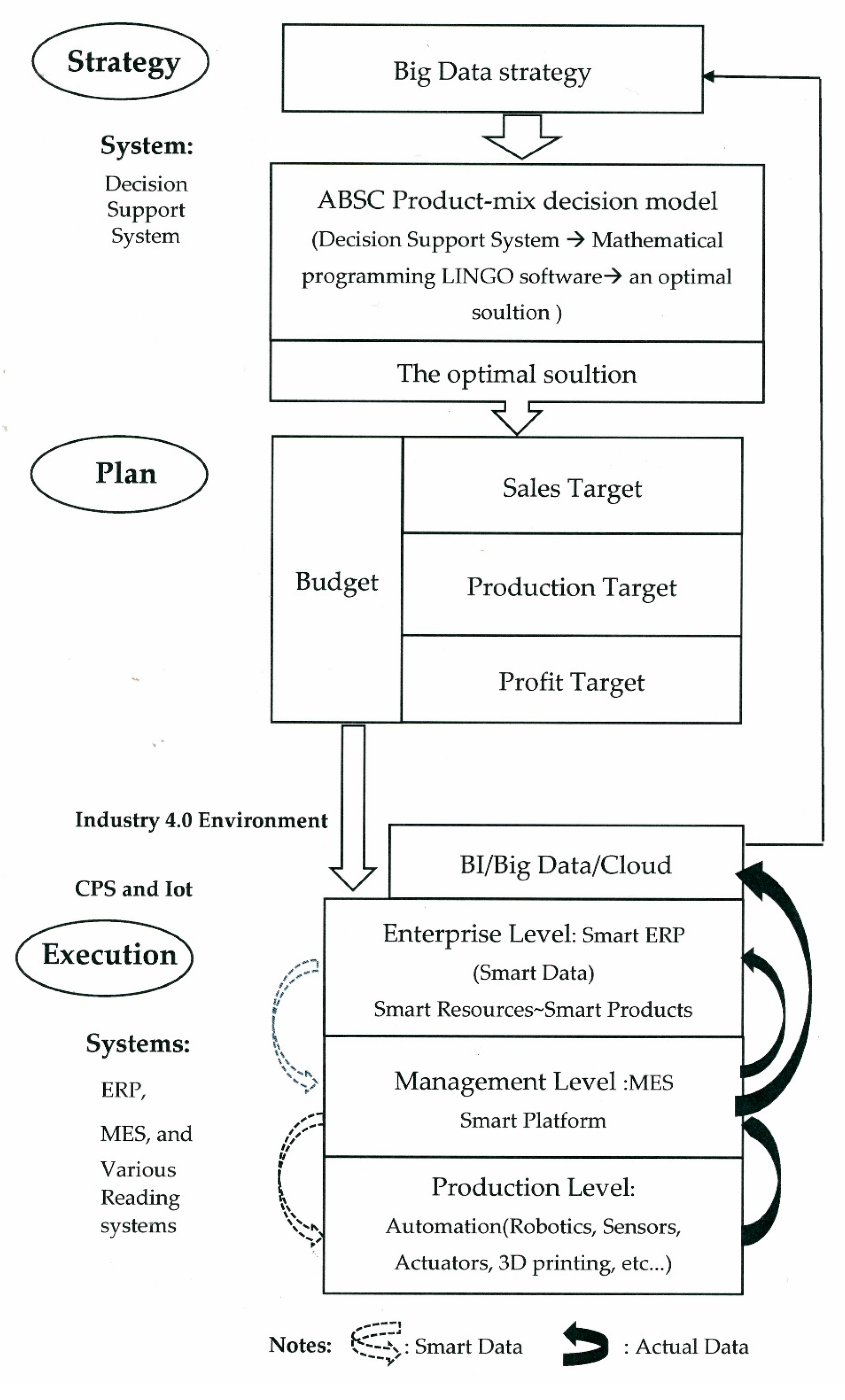
3.2.1. The Simulation of Production Strategies
3.2.2. Tools
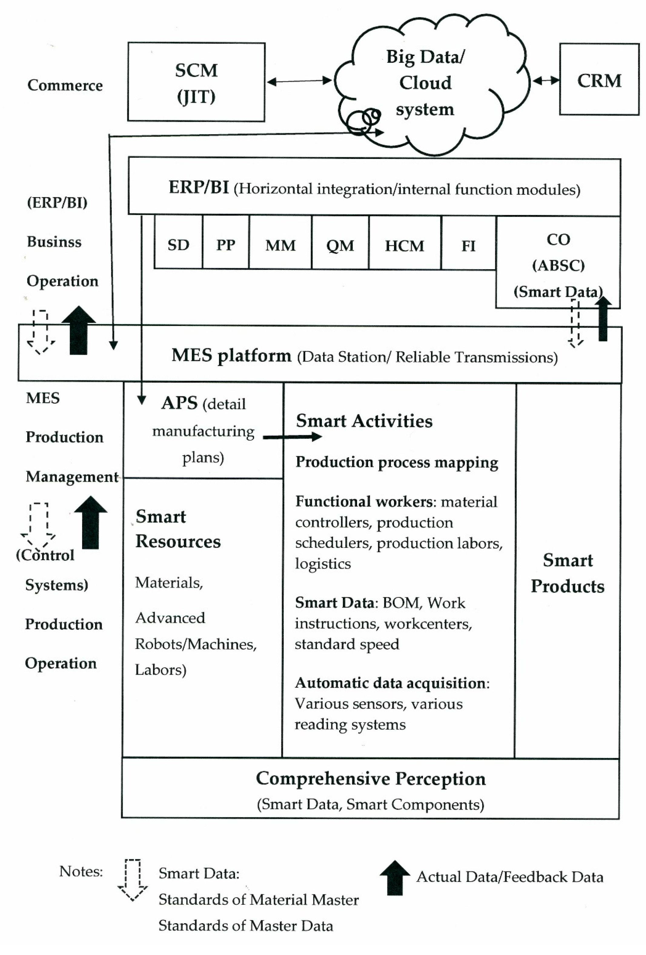
3.2.3. Information Technology for Horizontal and Vertical Integration
3.2.4. Machine-to-Machine Communication
3.3. ABSC Application in a Digital Manufacturing
3.4. ABSC Definition and Various Cost Calculation
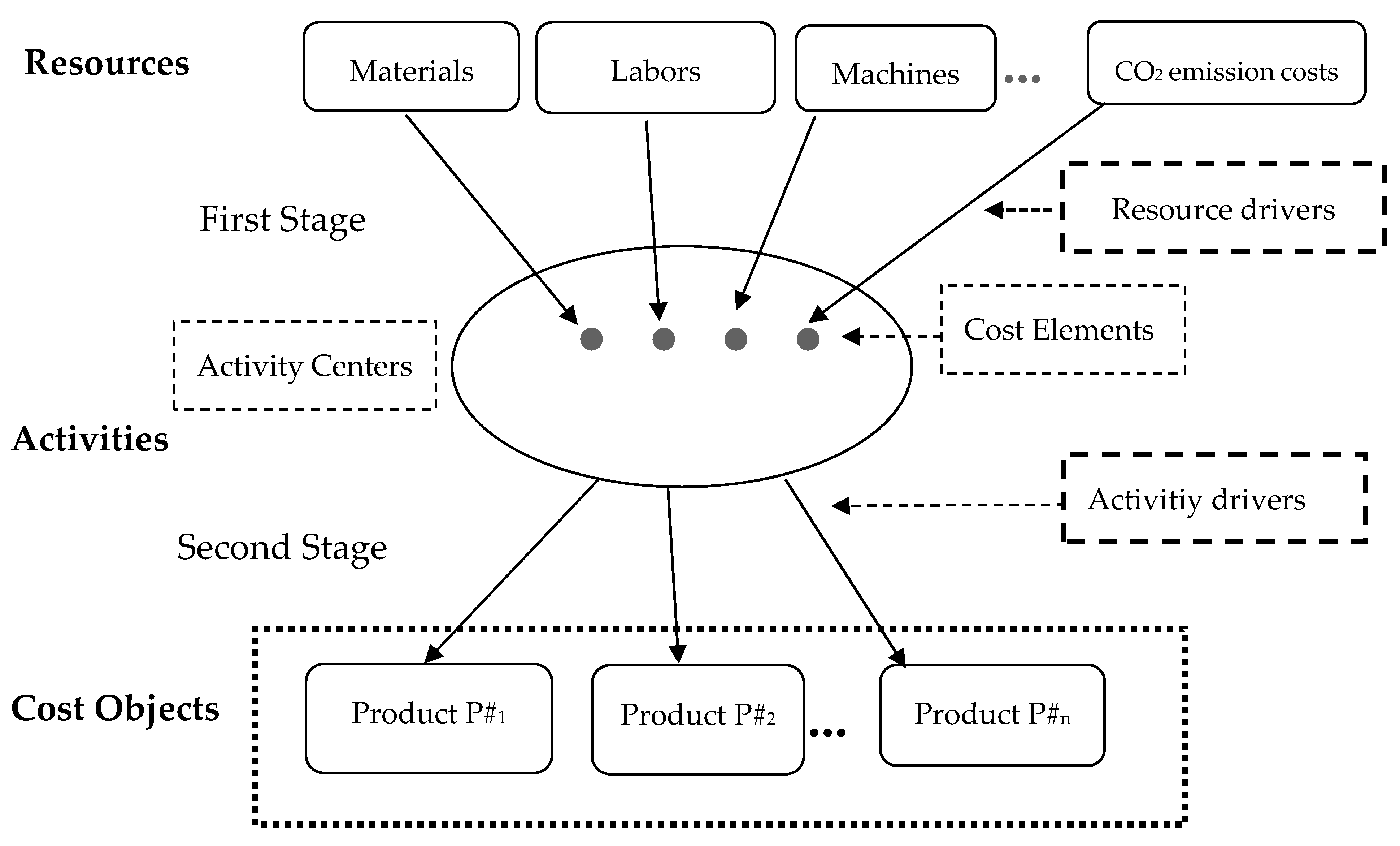
- Step 1. Calculating Resource Costs: The various resources used in a factory may include direct materials, direct laborers, machine hours, and other resources [3,6,28]. Resource costs are calculated using the quantity standards of the Material Master and Master Data [2] in the production process, as well as the standard of each resource unit price [7,8,28]. All detailed quantity data throughout the whole operation process can automatically be summed up for each resource element and then be tracked to its processes. As a result, resource costs can be calculated immediately in a smart ERP system.
- Step 2. Tracing Resource Costs to Activities: According to the various automatic data acquisitions in the data processes, some direct resource costs can automatically be traced to specific activities if a resource is consumed only by the specific activity [15,18,27]. Otherwise, the resource cost should be assigned to activities that consume the resource by an appropriate resource drive [2,10,27].
- Step 3. Standardized Activity Costs: An activity may be related to more than one process; thus, its indirect costs will be distributed to the related processes in the MES system [2,15,23]: For example, inspecting incoming material, moving materials, and indirect labor costs; maintaining and repairing machines; and other costs that are beneficial to all the manufacturing processes [15]. In other words, standardized activity costs can be traced to their related activities and processes [2,10,15], and the cost of each activity can be automatically calculated by adding the costs of the resource elements assigned to the activity [7,10,15]. In the new manufacturing era, mass customization is the key focus of manufacturing processes. Traditional standard costing should be changed to setting the detailed standards for elementary cost elements [2,15,18]. Thus, we will have the standard cost rate for each activity executed in the productions system. The standard cost of a specific product unit will be calculated by adding the products with standard activity cost rates and standard activity driver quantities consumed by this specific product unit [15,23,28].
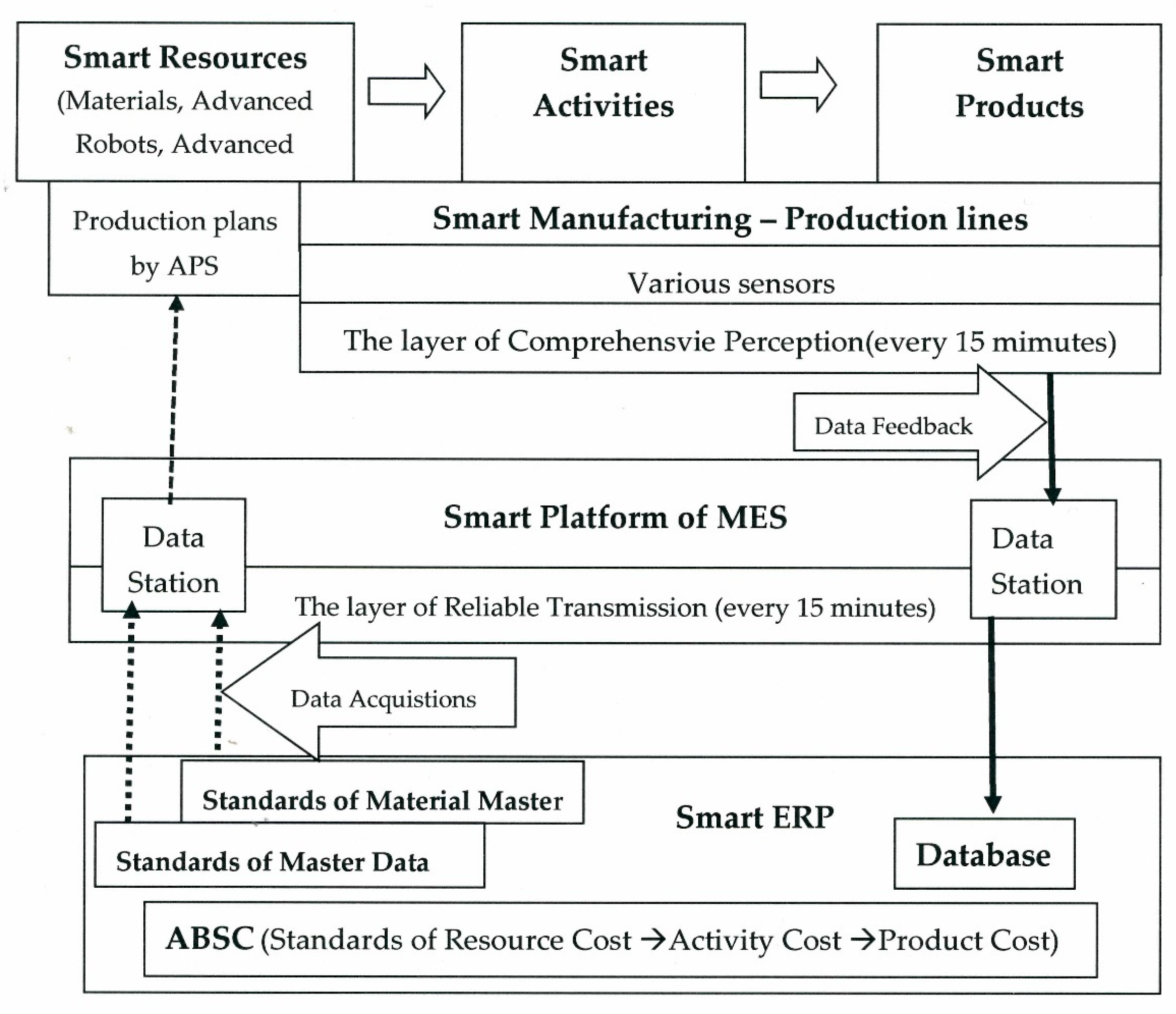
3.5. ABSC in ERP and linking MES in A Smart Factory
4. Formulation of an ABSC Product-Mix Decision Model for a Steel Factory
4.1. Process Descriptions and Cost Categories for the ABSC Mixed Decision Model for a Steel Factory
- Material cost: The purchase of steel-scrap raw materials should be based on the needs of EAF to clean, cut, and fracture for finishing all kinds of different sizes. The available steel-scrap will be poured into the hopper of EAF according to size in order for the EAF to be fully loaded and then will start the production of P#1 products.
- Labor cost: Including personnel normal and overtime costs;
- Electrical power cost: Including the high electrical bills for EAF, etc.;
- CO2 emission cost: Environmental and social costs in the form of a carbon tax for environmental protection;
- Machine cost: Machines and equipment are fixed costs in each process;
- Other indirect costs (overhead): With the exception of the above 1–5 costs in this subsection, other indirect costs per product are calculated as a percentage of the total amount sold for each product.
4.2. Assumptions
- The revenue includes steel products and slag byproducts;
- The direct raw material cost of steel-scrap with different purity levels and recycled materials for byproducts are assumed;
- Direct labor is related to the time of the production machine;
- The model complies with government policies, including direct labor overtime and tax cost for carbon dioxide emission;
- The direct costs include direct materials, machines, CO2 emission, labor, and electrical power costs;
- The machine cost of each process is fixed, regardless of any special overtime;
- The variable costs of other indirect costs are based on the total sales percentage for each product.
4.3. Notations
| Ω | The total profit; |
| P#i | The notation of products; |
| Pi | The sales unit price of Product i; |
| Qi | The sales quantity of the products (P#i); |
| USi | The sales upper quantity limit constraint of Product i; |
| LSi | The sales lower quantity limit constraints of Product i; |
| S1, S2 | The notations for the byproducts for both slag (S1) and steel-scrap (S2); |
| Qp | The selling quantity of the byproduct; |
| K1 | The unit sales price of the byproduct; |
| B | The amount of input per batch of steel-scrap in the steelmaking process; |
| Xj | The number of batches of steel-scrap of the jth level purity in a period; |
| Mj | The purchase of steel-scrap of the jth level steel purity; |
| Mcj | The unit purchase cost of the jth level steel-scrap; |
| M2r | The output of the steel-scrap byproduct (S2) in a period |
| Mc2r | The unit cost of the steel-scrap byproduct (S2); |
| Rj, Rj’ | The output of each batch of P#1 using the steel-scrap of the jth steel purity level; Rj’ is the output by enhancing the steel purity of steel-scrap for more value; |
| Ti | The output of the ith product after the steelmaking process; |
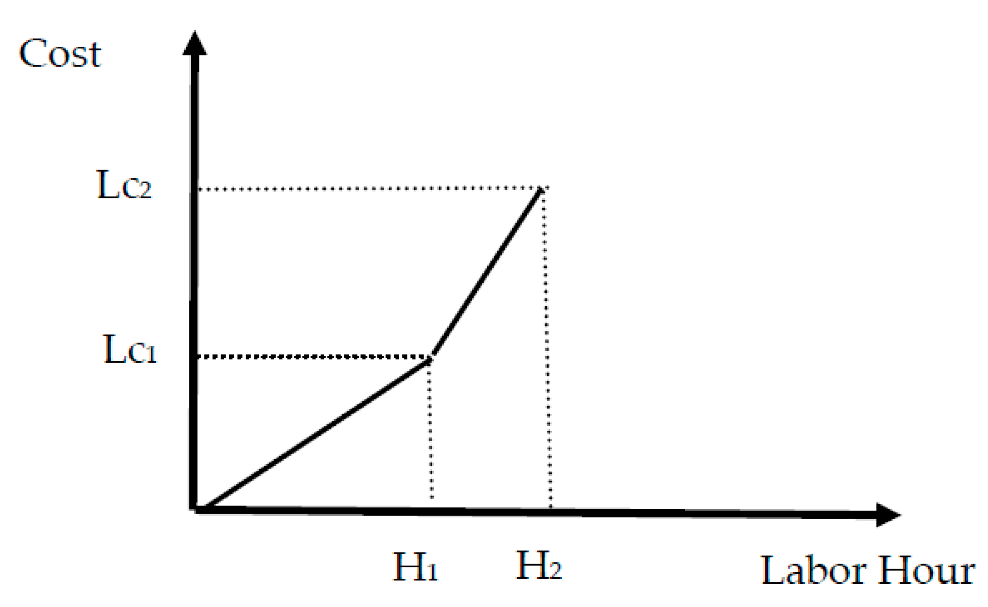
| H, H1, H2 | The total labor hours (H) including the normal hours (H1) and overtime hours (H2); |
| h1, h2, h3 | The direct labor hours for each batch (h1) in the steelmaking process and other processes for direct labor hours are per mt = 1000 kg (h2 and h3), including in the steel forging process and beam pressing process; |
| Lc, Lc1, Lc2 | The total direct labor costs (Lc) including the normal (Lc1) and overtime (Lc2) direct labor costs; |
| η1, η2 | (η1, η2) is an SOS1 (special ordered set of type 1) set of 0–1 variables within which exactly one variable must be nonzero (Williams 1985); |
| μ0, μ1, μ2 | (μ0, μ1, μ2) is an SOS2 (special ordered set of type 2) set of non-negative variables within which at most two adjacent variables, in the order given to the set, can be nonzero (Williams 1985); |
| θ1 | The wage rate for normal direct labor hours; |
| θ2 | The wage rate for overtime direct labor hours; |
| nh | The working hours per working day; |
| nd | The working days within a period; |
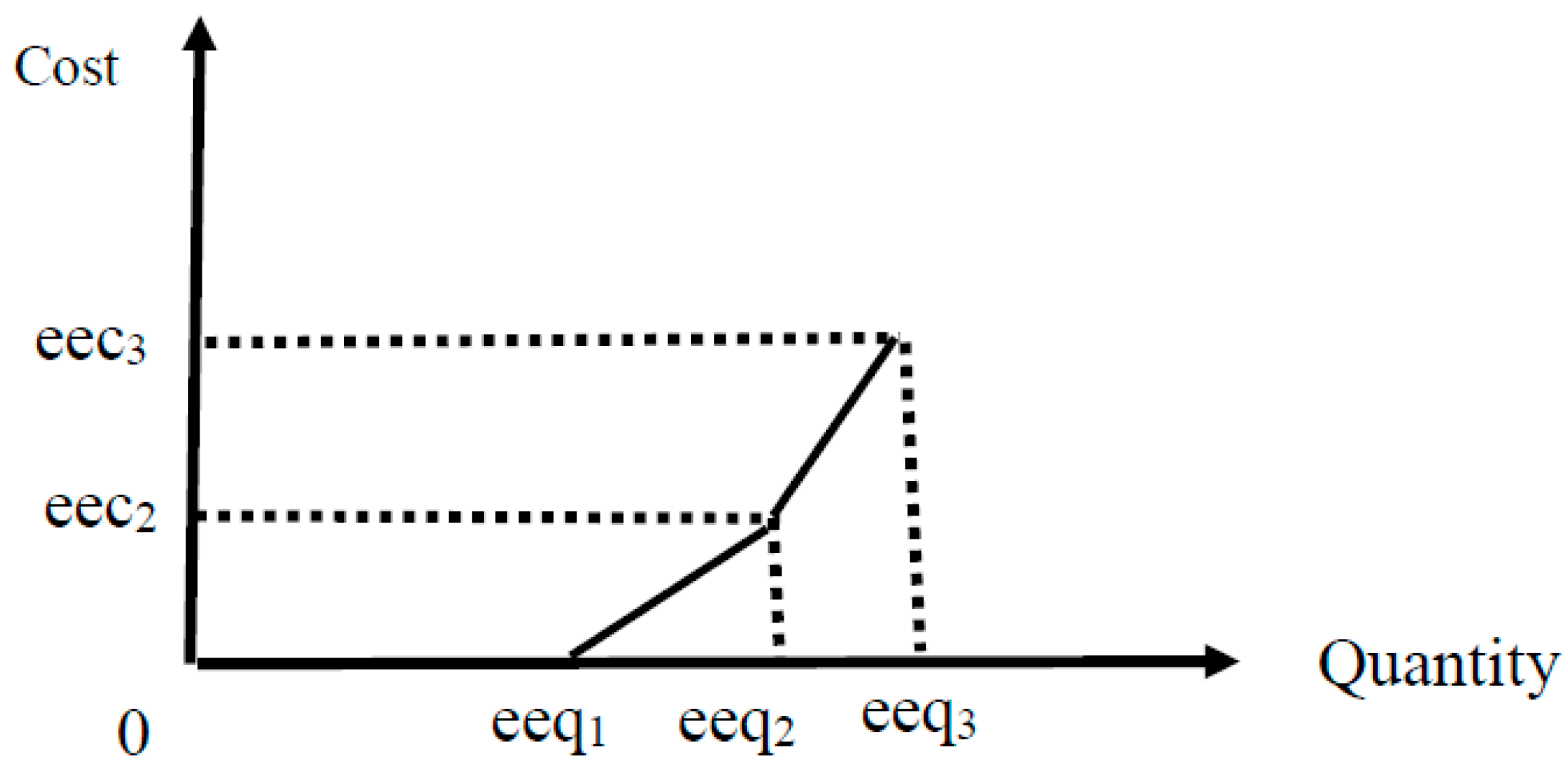
| eecb | The total CO2 emission cost; |
| eeqb | The total quantities of CO2 emission; |
| γ1, γ2, γ3 | An SOS1 (special ordered set of type 1) set of 0–1 variables within which exactly one variable must be nonzero (Williams 1985); |
| ψ0, ψ1, ψ2, ψ3 | An SOS2 (special ordered set of type 2) set of non-negative variables within which at most two adjacent variables, in the order given to the set, can be nonzero (Williams 1985); |
| cr | The carbon footprint calculated from production batches, which generate the quantity of cr mts carbon footprint emissions; |
| rb | The carbon tax rates including a free (r1) tax rate and USD2 (r2) and USD9(r3) carbon tax rates per mt; |
| Fh1, Fh2, Fh3 | The machine hours for each process; |
| Dci | The total direct electricity power cost including batch level in process 1 and unit level in Processes 2 and 3; |
| Du | The unit cost of 1 KW of electricity power; |
| Dn1, Dn2, Dn3 | The electrical power consumed by processes 1, 2, and 3 are Dn1, Dn2, and Dn3, respectively; |
| Fi | All machine costs in each process are fixed; |
| Oci and pri | Other indirect cost (Oci) for product i; allocating its cost based on the percentage of revenue of product i (pri). |
4.4. Mathematical Programming Model
4.4.1. The Model
| Maximize Ω = | (A) Sales amount (A1. Steel products + A2. Slag byproduct) |
| (B) Direct material cost (B1. Steel-scrap − B2. Recycling the byproduct of steel-scrap) | |
| (C) Direct labor cost (C1. Normal cost + C2. Overtime cost) | |
| (D) Direct electrical power cost | |
| (E) Direct machine cost | |
| (F) CO2 emission (Environmental and social cost) | |
| (G) Other indirect cost |
- A. Product sales upper limit constraintsQi ≦ USi
- Product sales lower limit constraintsQi ≧ LSi
- B1. Direct material quantity constraints
- C. Direct labor hour constraintsH = H1μ1 + H2μ2,μ1 − η1 − η2 ≦ 0,μ2 − η2 ≦ 0,η1 + η2 = 1, η1,η2 = 0,1,
- E. Machine hour constraints
- F. CO2 emission constraintseeqb = eeq1*ψ1 + eeq2*ψ2 + eeq3*ψ3γ1 + γ2 + γ3 = 1, γ1,γ2,γ3 = 0, 1
4.4.2. Sales Amount
4.4.3. Direct Material Cost
4.4.4. Direct Labor Cost
4.4.5. Direct Electricity Power Cost
4.4.6. Machine Costs
4.4.7. CO2 Emission Costs
4.4.8. Other Indirect Cost
5. Illustrative Case Study and Discussion
5.1. Sales Amount
5.2. Direct Material
5.2.1. Purchasing the Recycling Materials of Steel-Scrap and Producing Products
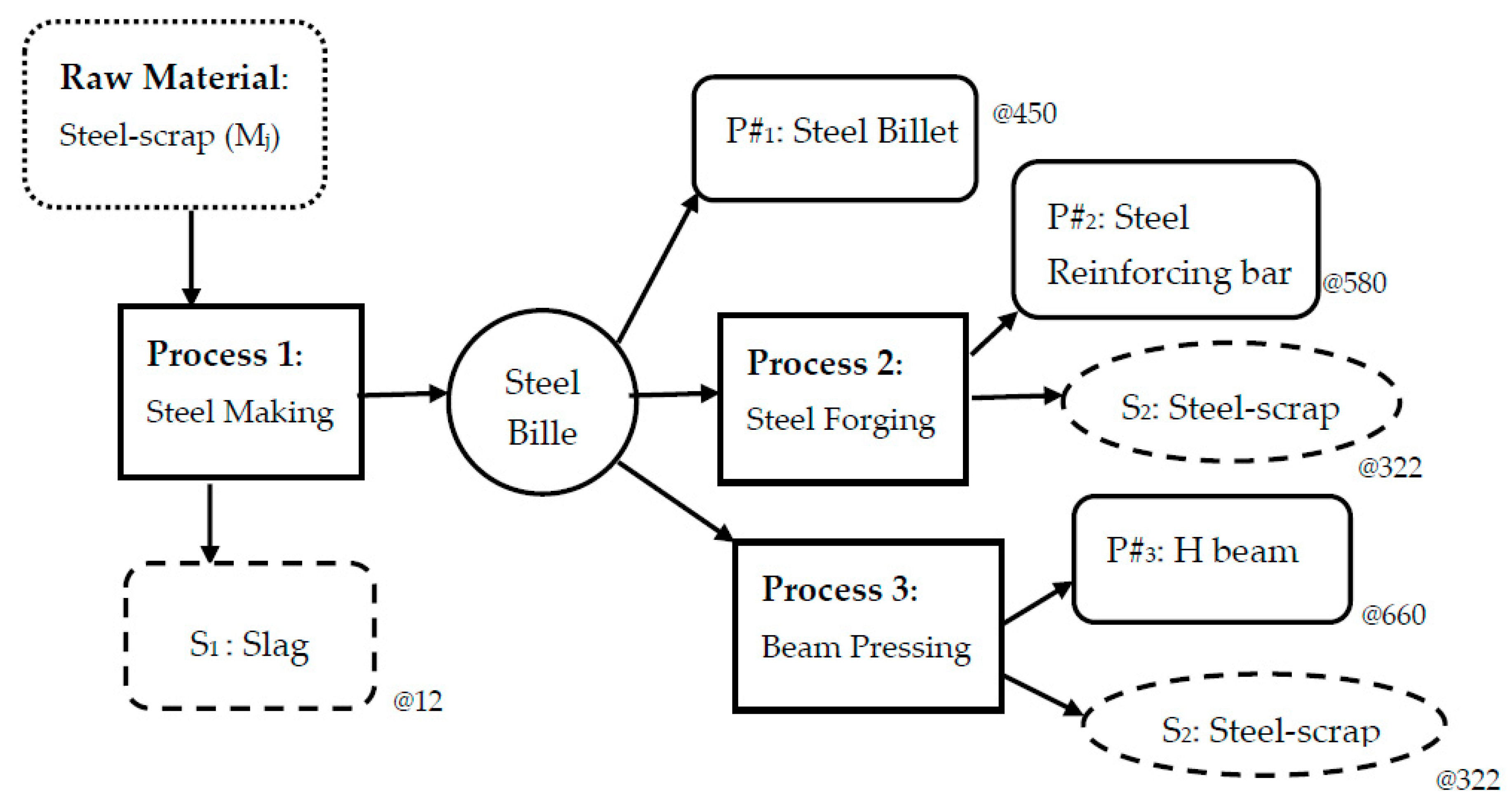
- Assume that producing P#1 can use three kinds of direct materials—steel-scrap Mj (M1, M2, and M3). The input material of product P#2 in Process 2 and P#3 in Process 3 come only from the P#1 (semi-manufactured goods called P#1). We also assume that the plant needs three main activities to produce these three products (P#1, P#2, and P#3), as shown in Figure 5 in Section 4.1.
- In process 1, inputting the steel-scrap of Mj into the EAF is for the production of P#1 and S1. P#1, which not only can be sold but also can produce other products (P#2 and P#3). For other products, meaning the semi-manufactured goods, P#1 must be transferred to other processes; one into Process 2 for producing P#2, another into Process 3 for producing P#3. Additionally, byproduct S2 will be produced in two Processes, namely, 2 and 3. The byproduct S2 will become a recycled material of steel-scrap, just as the M2r, and assume that the unit cost of Mc2r is equal to USD322 each mt.
- For the production of P#1, the purchase of three kinds of steel-scrap recycled materials Mj (M1, M2, and M3) are divided into 3 steel purity levels of the M1 lowest, M2 middle, and M3 highest levels, and the unit costs are USD300 (Mc1), USD317 (Mc2), and USD330 (Mc3), respectively. However, different levels of steel purity per batch (B = 100) will affect the yield of P#1 and S1 in Process 1, which range from 88, 91, to 94 mts and from 12, 9, to 6 mts, respectively.
5.3. Direct Labor
5.4. Electrical Power Cost
5.5. Machine Hours and Cost
5.6. CO2 Emission Quantity and Cost
5.7. Other Indirect Costs
5.8. The Optimal Solution
6. Three Cases on Enhancing the Quality of Steel-Scrap
6.1. Optimal Solution for Cases 1–4
6.2. Further Analysis
7. Summary and Conclusions
Author Contributions
Funding
Acknowledgments
Conflicts of Interest
References
- Qin, J.; Liu, Y.; Grosvenor, R. A Categorical Framework of Manufacturing for Industry 4.0 and Beyond. Procedia CIRP 2016, 52, 173–178. [Google Scholar] [CrossRef]
- Kletti, J. Manufacturing Execution System-MES; Springer: Berlin/Heidelberg, Germany; New York, NY, USA, 2007; pp. 61–78. [Google Scholar]
- Tsai, W.-H.; Yang, C.-H.; Chang, J.-C.; Lee, H.-L. An-Activity-Based Costing Decision Model for Life Cycle Assessment in Green Building Projects. Eur. J. Oper. Res. 2014, 238, 607–619. [Google Scholar] [CrossRef]
- Wikipedia. Steelmaking. Available online: https://en.m.wikipedia.org/wiki/Steelmaking (accessed on 23 January 2019).
- American Iron and Steel Institute. Steel Production, Recycling. Available online: http://www.steel.org/about-aisi/industry-profile.aspx (accessed on 23 January 2019).
- Tsai, W.-H. Activity-Based Costing Model for Joint Products. Comput. Ind. Eng. 1996, 31, 725–729. [Google Scholar] [CrossRef]
- Tsai, W.-H. Project Management Accounting Using Activity-Based Costing Approach. In The Handbook of Technology Management; Bidgoli, H., Ed.; John Wiley & Sons, Inc.: Hoboken, NJ, USA, 2010; Volume 1, pp. 469–488. [Google Scholar]
- Tsai, W.-H. A technical note on using work sampling to estimate the effort on activities under activity-based costing. Int. J. Prod. Econ. 1996, 43, 11–16. [Google Scholar] [CrossRef]
- Wagner, T.; Herrmann, C.; Thiede, S. Industry 4.0 impacts on lean production systems. Procedia CIRP 2017, 63, 125–131. [Google Scholar] [CrossRef]
- Bedolla, J.S.; D’Antonio, G.; Chiabert, P. A novel approach for teching IT tools with Lerning Factories. Procedia Manuf. 2017, 7, 175–181. [Google Scholar] [CrossRef]
- Liu, C.; Xu, X. Cyber-Physical Machine Tool—The Era of Machine Tool 4.0. Procedia CIRP 2017, 63, 70–75. [Google Scholar] [CrossRef]
- Pacaux-Lemoine, M.P.; Trentesaux, D.; Rey, G.Z.; Millot, P. Designing intelligent manufacturing systems through Human-Machine Cooperation principles: A human-centered approach. Comput. Ind. Eng. 2017, 111, 581–595. [Google Scholar] [CrossRef]
- Gašová, M.; Gašo, M.; Štefánik, A. Advanced industrial tools of ergonomics based on Industry 4.0. Procedia Eng. 2017, 192, 219–224. [Google Scholar] [CrossRef]
- Santos, M.Y.; e Sá, J.O.; Andrade, C.; Lima, F.V.; Costa, E.; Costa, C.; Martinho, B.; Galvão, J. A Big Data system supporting Bosch Braga Industry 4.0 strategy. Int. J. Inf. Manag. 2017, 36, 750–760. [Google Scholar] [CrossRef]
- Moutaz, H.; Ahmed, E. The Readiness of ERP Systems for the Factory of the Future. Procedia Comput. Sci. 2015, 64, 721–728. [Google Scholar]
- Grundstein, S.; Freitag, M.; Scholz-Reiter, B. A new method for autonomous control of complex job shops- Integrating order release, sequencing and capacity control to meet due dates. J. Manuf. Syst. 2017, 42, 11–28. [Google Scholar] [CrossRef]
- Kans, M.; Ingwald, A. Business Model Development towards Service Management 4.0. Procedia CIRP 2016, 47, 489–494. [Google Scholar] [CrossRef]
- Wang, S.; Wan, J.; Zhang, D.; Li, D.; Zhang, C. Towards smart factory for industry 4.0: A self-organized multi-agent system with big data based feedback and coordination. Comput. Netw. Volume 2016, 101, 158–168. [Google Scholar] [CrossRef]
- Stock, T.; Seliger, G. Opportunities of Sustainable Manufacturing in Industry 4.0. Procedia CIRP 2016, 40, 536–541. [Google Scholar] [CrossRef]
- Becker, T.; Stern, H. Future trends in human work area design for cyber-physical production system. Procedia CIRP 2016, 57, 404–409. [Google Scholar] [CrossRef]
- Wikipedia. Paris Agreement. Available online: https://en.wikipedia.org/wiki/paris agreement (accessed on 15 March 2018).
- Tung Ho Steel Enterprise Corp. Profile, CSR, Products. Available online: http://www.tunghosteel.com/EN/HomeEg/about/intro (accessed on 23 January 2019).
- Tsai, W.-H.; Lin, S.-J.; Liu, J.-Y.; Lin, W.-R.; Lee, K.-C. Incorporating life cycle assessments into building project decision-making: An energy consumption and CO2 emission perspective. Energy 2011, 36, 3022–3029. [Google Scholar] [CrossRef]
- Bauerdick, C.J.; Helfert, M.; Menz, B.; Abele, E. A common sofrware Framework for Energy Data Based Monitoring and Controlling for Machine power Peak Reduction and Workpiece Quality Improvements. Procedia CIRP 2017, 61, 359–364. [Google Scholar] [CrossRef]
- Chen, J.-Y.; Tai, K.-C.; Chen, G.-C. Application of programmable Logic Controller to Build-up an Intelligent Industry 4.0 Platform. Procedia CIRP 2017, 63, 150–155. [Google Scholar] [CrossRef]
- Rudolph, J.P.; Emmelmann, C. A Cloud-Based Platform for Automted Order Processing in Additive Manufacturing. Procedia CIRP 2017, 63, 412–417. [Google Scholar] [CrossRef]
- Chen, K.-C.; Lien, S.-Y. Machine-to-machine communications: Technologies and challenges. Ad Hoc Netw. 2014, 18, 3–23. [Google Scholar] [CrossRef]
- Tsai, W.-H.; Lin, T.-W.; Chou, W.-C. Integrating Activity-Based Costing and Environmental Cost Accounting Systems: A Case Study. Int. J. Bus. Syst. Res. 2010, 4, 186–208. [Google Scholar] [CrossRef]
- Tsai, W.-H.; Lin, T.W. A Mathematical Programming Approach to Analyze the Activity-Based Costing Product-Mix Decision with Capacity Expansions. In Applicatios of Management Science; Lawrence, K.D., Ed.; JAI Press Inc.: Greenwich, CT, USA, 2004; Volume 11, pp. 161–176. [Google Scholar]
- Chinnathai, M.K.; Günther, T.; Ahmad, M.; Stocker, C.; Richter, L.; Schreiner, D.; Vera, D.; Reinhart, G.; Harrison, R. An application of physical flexibility and software reconfigurability for the automation of battery module assembly. Procedia CIRP 2017, 63, 604–609. [Google Scholar] [CrossRef]
- de Sampaio, R.J.; Wollmann, R.R.; Vieira, P.F. A flexible production planning for rolling-horizons. Int. J. Product. Econ. 2017, 190, 31–36. [Google Scholar] [CrossRef]
- de Man, J.C.; Strandhagen, J.O. An Industry 4.0 research agenda for sustainable business models. Procedia CIRP 2017, 63, 721–726. [Google Scholar] [CrossRef]
- Poonpakdee, P.; Koiwanit, J.; Yuangyai, C. Decentralized Network Building Change in Large Manufacturing Companyies towards Industry 4.0. Procendia Comput. Sci. 2017, 110, 46–53. [Google Scholar] [CrossRef]
- Meissner, H.; Ilsen, R.; Aurich, J.C. Analysis of control architectures in the context of Industry 4.0. Procedia CIRP 2017, 62, 165–169. [Google Scholar] [CrossRef]
- Kolsch, P.; Herder, C.F.; Zimmermann, V.; Aurich, J.C. A novel concept for the development of availability- oriented business models. Procedial CIRP 2017, 64, 340–344. [Google Scholar] [CrossRef]
- Schlegel, A.; Langer, T.; Putz, M. Developing and harnessing the potential of SMEs for eco-efficient flexible production. Procedia Manuf. 2017, 9, 41–48. [Google Scholar] [CrossRef]
- Majstorovic, V.; Stojadinovic, S.; Zivkovic, S.; Djurdjanovic, D.; Jakovljevic, Z.; Gligorijevic, N. Cyber-Physical Manufacturing Metrology Model (CPM) for sculptured surfaces- Turbine Blade Application. Procedia CIRP 2017, 63, 658–663. [Google Scholar] [CrossRef]
- Lee, J.; Bagheri, B.; Kao, H.A. A Cyber-Physical Systems architecture for Industry 4.0-based manufacturing systems. Manuf. Lett. 2015, 3, 18–23. [Google Scholar] [CrossRef]
- Li, H.; Parlikad, A.K. Social Internet of Industrial Things for Industrial and Manufacturing Assets. IFAC 2016, 49, 208–213. [Google Scholar]
- Functional SAP ERP Modules. SAP ERP Modules: Complete List of SAP ERP Modules. Available online: https://solutiondots.com/blog/sap-erp-modules/ (accessed on 13 January 2019).
- Tsai, W.-H.; Yang, C.-H.; Huang, C.-T.; Wu, Y.-Y. The Impact of the Carbon Tax Policy on Green Building Strategy. J. Environ. Plan. Manag. 2017, 60, 1412–1438. [Google Scholar] [CrossRef]
- Tsai, W.-H.; Tsaur, T.-S.; Chou, Y.-W.; Liu, J.-Y.; Hsu, J.-L.; Hsieh, C.-L. Integrating the Activity-Based Costing System and Life-Cycle Assessment into Green Decision Making. Int. J. Prod. Res. 2015, 53, 451–465. [Google Scholar] [CrossRef]
- Tsai, W.-H.; Chang, J.-C.; Hsieh, C.-L.; Tsaur, T.-S.; Wang, C.-W. Sustainability Concept in Decision-Making: Carbon Tax Consideration for Joint Product Mix Decision. Sustainability 2016, 8, 1232. [Google Scholar] [CrossRef]
- Tsai, W.-H. A Green Quality Management Decision Model with Carbon Tax and Capacity Expansion under Activity-Based Costing (ABC)—A Case Study in the Tire Manufacturing Industry. Energies 2018, 11, 1858. [Google Scholar] [CrossRef]
- Tsai, W.-H. Carbon Taxes and Carbon Rights Cost Analysis for the Tire Industry. Energies 2018, 11, 2121. [Google Scholar] [CrossRef]
- Tsai, W.-H.; Lu, Y.-H. A Framework of Production Planning and Control with Carbon Tax under Industry 4.0. Sustainability 2018, 10, 3221. [Google Scholar] [CrossRef]
- Tsai, W.-H. Green Production Planning and Control for the Textile Industry by Using Mathematical Programming and Industry 4.0 Techniques. Energies 2018, 11, 2072. [Google Scholar] [CrossRef]
- Tsai, W.-H.; Jhong, S.-Y. Carbon Emission Cost Analysis with Activity-Based Costing. Sustainability 2018, 10, 2872. [Google Scholar] [CrossRef]
- Tsai, W.-H.; Jhong, S.-Y. Production Decision Model with Carbon Tax for the Knitted Footwear Industry under Activity-Based Costing. J. Clean. Prod. 2019, 207, 1150–1162. [Google Scholar] [CrossRef]
- Tsai, W.-H.; Lai, S.-Y. Green Production Planning and Control Model with ABC under Industry 4.0 for the Paper Industry. Sustainability 2018, 10, 2932. [Google Scholar] [CrossRef]
- Tsai, W.-H.; Chu, P.-Y.; Lee, H.-L. Green Activity-Based Costing Production Planning and Scenario Analysis for the Aluminum-Alloy Wheel Industry under Industry 4.0. Sustainability 2019, 11, 756. [Google Scholar] [CrossRef]

| Traditional Activity-Based Costing (ABC) | Technological Development | Innovative ABSC |
|---|---|---|
| Resources |
| Smart resources:
|
| Activities | Smart Activities: Smart resource into operation | |
| Products (Cost Objects) | Smart Products: | |
| Using system: Enterprise Resource Planning (ERP) ERP data, including all standard costs |
| |
| ABC/ABSC Application: product-mix decision model Method: various constraints and mathematical programming Using strategic system: Decision Support System Results: an optimal decision solution for maximizing profit | ||
| ABSC application in the Big Data of Industry 4.0: Recommendations:
| ||
| Description | Material (Mj) for P#1 | Products (P#i/S1) | ||||
|---|---|---|---|---|---|---|
| Sales | P#1/S1 | P#2 | P#3 | |||
| Demand (Qi)/mts | 2000 ≦ Q1 ≦ 4000 | Q2 ≥ 3500 | Q3 ≥ 3500 | |||
| Products price (Pi)/USD | $450 | $580 | $660 | |||
| Byproduct price (K1)/USD | $12 | |||||
| Direct Material | M1 | M2 | M3 | |||
| Unit price (Mcj)/mt/USD | $300 | $317 | $330 | |||
| Total batches (Xj)/100mts | X1 ≦ 65 | X2 ≦ 65 | X3 ≦ 65 | |||
| Output P#1(Ri)/1 batch (B) | R1 = 88 | R2 = 91 | R3 = 94 | |||
| Output S1(B-Ri)/1 batch (B) | 12 | 9 | 6 | |||
| P#1 for selling Products (Ti)/mt | 1 | 0.96 | 0.98 | |||
| Transfer P#1 (Qi/Ti)/ mts to others process | Q1/T1 | Q2/T2 | Q3/T3 | |||
| Recycling the S2 byproduct (Qi/Ti) − Qi/ mts | (Q2/T2)-Q2 | (Q3/T3)-Q3 | ||||
| Unit S2 byproduct cost (Mc2r)/mt/USD | $322 | $322 | ||||
| Direct Labor | ||||||
| Cost/USD | Lc1 = $66,000; Lc2 = $105,600 | |||||
| Labor hours | H1 = 10,000; H2 = 14,000 | |||||
| Wage rate/USD | θ1 = $6.6; θ2 = 9.9 | |||||
| Electrical power | ||||||
| Each batch level 0.75 hours/KW | 45 | |||||
| Unit level hours/mt | 0.1 | 0.1 | ||||
| 1 KW (Du) cost/USD | 85 | 85 | 85 | |||
| Machine | ||||||
| Machine hours (Fhi) | Fh1 ≦ 176 | Fh2 = Q2 | Fh3 = Q3 | |||
| Machine cost (Fi)/USD | F1 = $100,000 | F2 = $50,000 | F3 = $150,000 | |||
| CO2 Emission | ||||||
| Carbon cost (eecb) | eec1 = $0; eec2 = $2000; eec3 = $29,000 | |||||
| Carbon Q’ty(eeqb) | eeq1 = 3000; eeq2 = 4000; eeq3 = 7000 | |||||
| Carbon rate (cr)/batch | cr = 40 | |||||
| Unit carbon (rb)/USD | r1 = $0; r2 = $2; r3 = $9; | |||||
| Other indirect costs | ||||||
| Oci | 3%*Q1*P1 | 5%*Q2*P2 | 5%*Q3*P3 | |||
| MAX Ω = {(450Q1 + 580Q2 + 660Q3) + 12 [X1(100 − 88) + X2(100 − 91) + X3(100 − 94)]} − {[100(X1300 + X2317 + X3330)] − [(Q2/0.96(1 − 0.96) + (Q3/0.98(1 − 0.98)]322} − (66,000μ1 + 105,600μ2) − (8545(X1 + X2 + X3) + 850.1*Q2 + 850.1*Q3)-300000-(0γ1 + 2000γ2 + 29,000γ3)-(450Q10.03 + 580Q20.05 + 660Q30.05) |
| Subject to sales Q1 ≧ 2000 Q1 ≦ 4000 Subject to direct material X1 * 88 + X2 * 91 + X3 * 94 − Q1 − Q2/0.96 − Q3/0.98 = 0 X1 ≦ 65 X2 ≦ 65 X3 ≦ 65 Subject to machine hours (X1 + X2 + X3) *(0.5 + 0.75) ≦ 176 Q2 ≧ 3500 Q3 ≧ 3500 Subject to direct labor (X1 + X2 + X3)*17.5 + Q21 + Q31 ≦ 10,000 μ1 + 14,000μ2 (X1 + X2 + X3)*17.5 ≦ 14822; μ0 − η1 ≦ 0; μ1 − η1 − η2 ≦ 0; μ2 − η2 ≦ 0; μ0 + μ1 + μ2 = 1; η1 + η2 = 1; Subject to CO2 Emission (X1 + X2 + X3)1000.4 = 3000γ1 + 4000γ2 + 7000γ3 ψ0 − γ1 , ψ1 − γ1 − γ2 , ψ2 − γ2 − γ3 , ψ3 − γ3 , ψ0 + ψ1 + ψ2 + ψ3 = 1, 0 ψ0,ψ1,ψ2,ψ3 ≦ 1, γ1 + γ2 + γ3 = 1 γ1,γ2,γ3 = 0, 1 |
| Optimal decision solution for Case 1 Ω = 1,824,129, Q1 = 2002, Q2 = 3504, Q3 = 7105, X1 = 11, X2 = 64, X3 = 65, μ1 = 0.23525, μ2 = 0.76475, η2 = 1, ψ2 = 0.4666667, ψ3 = 0.5333333, γ3 = 1 |
| Description | Material (Mj) for P#1 | Products (P#i) | ||||
|---|---|---|---|---|---|---|
| Sales: | P#1 | P#2 | P#3 | |||
| Maximum demand (Qi)/mt | 2002 | 3504 | 7105 | |||
| Byproduct Q’ty (Qp)/mt 1 | 1098 | |||||
| Selling unit price—product/USD | $450 | $580 | $660 | |||
| Selling unit price—byproduct/USD | $12 | |||||
| Direct material constraint: | ||||||
| Batch-level activity: | ||||||
| Direct material: | M1 | M2 | M3 | |||
| Cost/unit price/mt | $300 | $317 | $330 | |||
| Input total batches (100 mts/1 batch) | 11 | 64 | 65 | |||
| Output product 1 (P#1): (mts/ 1 batch) | 88 | 91 | 94 | |||
| P#1 for the P#i/mt | 1 | 0.96 | 0.98 | |||
| Transfer P#1 (qi) to the ith process/mts 2 | 2002 | 3650 | 7250 | |||
| Recycling the byproduct (M2r) of products 2 and 3/mt 3 | ||||||
| Direct labor constraint | 0 | 146 | 145 | |||
| Labor cost (P#1/P#2/P#3) 4 | ||||||
| Labor hours (P#1/P#2/P#3) 5 | $16,170 | $26,539 | $53,575.1 | |||
| Electrical power cost | 2450 | 3504 | 7105 | |||
| Batch-level cost 6 | $535,500 | |||||
| Unit-level cost 6 | $29,784 | $60,393 | ||||
| Direct machine constraint | ||||||
| Machine cost | $100,000 | $50,000 | $150,000 | |||
| Machine hours (batch/unit) | 175 | 3504 | 7105 | |||
| CO2 emission constraint | ||||||
| Batch-level mts 7 | 5600 | |||||
| Batch-level cost 8 | $16,400 | |||||
| Other indirect cost9 | $27,027 | $101,616 | $234,465 | |||
| Mcj | Mcj’ = Mcj + USD 8 | |||||
| Mc1 @300 | Mc2 @317 | Mc3 @330 | Mc1’ @308 | Mc2’ @325 | Mc3’ @338 | |
| P#1/Batch (100 mts) | ||||||
| Rj | Rj’ = Rj + 2 mts | |||||
| R1 | R2 | R3 | R1’ | R2’ | R3’ | |
| 88 | 91 | 94 | 90 | 93 | 96 | |
| Case 1 | 300 | 317 | 330 | |||
| Case 2 | 317 | 330 | 308 | |||
| Case 3 | 330 | 308 | 325 | |||
| Case 4 | 308 | 325 | 338 | |||
| Case | Profit | Sales quantity | Batches Xj | Direct Labor μw | CO2 emission ψe | ||||||||
|---|---|---|---|---|---|---|---|---|---|---|---|---|---|
| Ω | Q1 | Q2 | Q3 | X1 | X2 | X3 | μ1 | μ2 | ψ2 | ψ3 | γ3 | η2 | |
| 1 | 1,824,129 | 2002 | 3504 | 7105 | 11 | 64 | 65 | 0.23525 | 0.76475 | 0.466667 | 0.533333 | 1 | 1 |
| 2 | 1,874,986 | 2002 | 3504 | 7056 | 65 | 16 | 59 | 0.24750 | 0.75250 | 0.466667 | 0.533333 | 1 | 1 |
| 3 | 1,885,635 | 2001 | 3504 | 7252 | 11 | 65 | 64 | 0.19850 | 0.80150 | 0.466667 | 0.533333 | 1 | 1 |
| 4 | 1,909,646 | 2002 | 3504 | 7350 | 21 | 54 | 65 | 0.17400 | 0.82600 | 0.466667 | 0.533333 | 1 | 1 |
| Case | Assumptions Mcj→Mcj’ (USD) | Quantity (mt) | Sales Amount (USD) | Material Cost (USD) | Costs (USD) | ||||||||
|---|---|---|---|---|---|---|---|---|---|---|---|---|---|
| (1) Mc1 | (2) Mc2 | (3) Mc3 | (4) M2r | (5) Qp | (6) Pi*Qi | (7) K1*Qp | (8) Mcj*Xj*B | (9) M2r*Mc2r | (10) Lc | (11) Dci | (12) eecb | (13) Oci | |
| 1 | 300 | 317 | 330 | 291 | 1098 | 7,622,520 | 13,176 | 4,503,800 | 93,702 | 96,284 | 625,677 | 16,400 | 363,108 |
| 2 | 308 | 317 | 330 | 290 | 1148 | 7,590,180 | 13,776 | 4,456,200 | 93,380 | 95,799 | 625,260 | 16,400 | 361,491 |
| 3 | 308 | 325 | 330 | 294 | 949 | 7,719,090 | 11,388 | 4,563,300 | 94,668 | 97,739 | 626,926 | 16,400 | 367,946 |
| 4 | 308 | 325 | 338 | 296 | 848 | 7,784,220 | 10,176 | 4,598,800 | 95,312 | 98,710 | 627,759 | 16,400 | 371,193 |
| Description | Case 1 | Case 2 | Case 3 | Case 4 | ||||
|---|---|---|---|---|---|---|---|---|
| Total sales (A=A1+A2) | 7,635,696 | 100.0% | 7,603,956 | 100% | 7,730,478 | 100% | 7,794,396 | 100% |
| Product sales (A1) | 7,622,520 | 99.8% | 7,590,180 | 99.8% | 7,719,090 | 99.9% | 7,784,220 | 99.9% |
| Byproduct sales (A2) | 13,176 | 0.2% | 13,776 | 0.2% | 11,388 | 0.1% | 10,176 | 0.1% |
| Direct material cost (B=B1-B2) | 4,410,098 | 57.8% | 4,362,820 | 57.4% | 4,468,632 | 57.8% | 4,503,488 | 57.8% |
| Purchasing material (B1) | 4,503,800 | 59.0% | 4,456,200 | 58.6% | 4,563,300 | 59.0% | 4,598,800 | 59.0% |
| Recycling material (B2) | 93,702 | 1.2% | 93,380 | 1.2% | 94,668 | 1.2% | 95,312 | 1.2% |
| Direct labor cost (C) | 96,284 | 1.3% | 95,799 | 1.3% | 97,739 | 1.2% | 98,710 | 1.3% |
| Electrical power cost (D) | 625,677 | 8.2% | 625,260 | 8.2% | 626,926 | 8.1% | 627,759 | 8.1% |
| Machine cost (E) | 300,000 | 3.9% | 300,000 | 3.9% | 300,000 | 3.9% | 300,000 | 3.8% |
| CO2 emission cost (F) | 16,400 | 0.2% | 16,400 | 0.2% | 16,400 | 0.2% | 16,400 | 0.2% |
| Other indirect cost (G) | 363,108 | 4.8% | 361,491 | 4.8% | 367,946 | 4.8% | 371,193 | 4.8% |
| Total profit (H=A-B-C-D-E-F-G) | 1,824,129 | 23.9% | 1,842,186 | 24.2% | 1,852,835 | 24.0% | 1,876,846 | 24.1% |
© 2019 by the authors. Licensee MDPI, Basel, Switzerland. This article is an open access article distributed under the terms and conditions of the Creative Commons Attribution (CC BY) license (http://creativecommons.org/licenses/by/4.0/).
Share and Cite
Tsai, W.-H.; Lan, S.-H.; Huang, C.-T. Activity-Based Standard Costing Product-Mix Decision in the Future Digital Era: Green Recycling Steel-Scrap Material for Steel Industry. Sustainability 2019, 11, 899. https://doi.org/10.3390/su11030899
Tsai W-H, Lan S-H, Huang C-T. Activity-Based Standard Costing Product-Mix Decision in the Future Digital Era: Green Recycling Steel-Scrap Material for Steel Industry. Sustainability. 2019; 11(3):899. https://doi.org/10.3390/su11030899
Chicago/Turabian StyleTsai, Wen-Hsien, Shu-Hui Lan, and Cheng-Tsu Huang. 2019. "Activity-Based Standard Costing Product-Mix Decision in the Future Digital Era: Green Recycling Steel-Scrap Material for Steel Industry" Sustainability 11, no. 3: 899. https://doi.org/10.3390/su11030899
APA StyleTsai, W.-H., Lan, S.-H., & Huang, C.-T. (2019). Activity-Based Standard Costing Product-Mix Decision in the Future Digital Era: Green Recycling Steel-Scrap Material for Steel Industry. Sustainability, 11(3), 899. https://doi.org/10.3390/su11030899