Temporal and Spatial Changes of Non-Point Source N and P and Its Decoupling from Agricultural Development in Water Source Area of Middle Route of the South-to-North Water Diversion Project

Abstract

The quantitative estimation of non-point source (NPS) pollution provides the scientific basis for sustainability in ecologically sensitive regions. This study combined the export coefficient model and Revised Universal Soil Loss Equation to estimate the NPS nitrogen (NPS-N) and NPS phosphorus (NPS-P) loads and then evaluated their relationship with Primary Industrial Output Value (PIOV) in the water source area of the middle route of South-to-North Water Diversion Project (SNWDP) for 2000–2015. The estimated results show that: (1) dissolved nitrogen (DN) load increased 0.55%, and dissolved phosphorus (DP) load decreased 4.60% during the 15 years. Annual loads of adsorbed nitrogen (AN) and adsorbed phosphorus (AP) increased significantly before 2005 and then decreased after 2005. Compared with 2000, AN and AP loads in 2015 significantly decreased by 32.72% and 30.81%, respectively. Hanzhong Basin and Ankang Basin are key areas for controlling dissolved pollution, and southern and northern regions are key areas for adsorbed pollution. (2) From 2000 to 2005, NPS pollutants and PIOV showed weak decoupling status. By 2015, NPS pollutants had strong decoupling from PIOV in most counties. (3) Land use has been the main source of NPS-N and NPS-P pollution, accounting for about 75% of NPS-N and 50% of NPS-P based on the average value over the study period. In the future, various measures—such as returning cropland to forest and reducing the number of livestock—could be adopted to reduce the risk of NPS pollution. NPS pollution caused by livestock was grown over the past 15 years and had not yet been effectively controlled, which still needs to be urgently addressed. Collecting ground monitoring data and revising parameters are effective means to improve the accuracy of simulation, which deserve further study. The results will also provide scientific support for sustainable development in similar regions.

1. Introduction

With living standards improving, people have higher demands for their living environments, in particular water quality. Simultaneously, water pollution caused by human activities is becoming increasingly prominent—it has aroused widespread concern worldwide [1,2]. Point source pollutants, mainly driven by industrial pollution, and non-point source (NPS) pollutants, mainly resulting from rural behaviors and runoff from urban areas where sewage treatment is insufficient, are the primary causes of water pollution [3]. Due to the attention received by the community, point source pollution has, for the most part, been effectively curbed, and NPS pollution has gradually become the dominant contributor to water pollution. Non-point source pollution has always been an important factor affecting water quality in the United States [4]. To solve the problem, since 1990, the United States government has invested over $100 million annually on average to solve the problem [5]. In Miksa City, Japan, 61.5% of the nitrogen load comes from non-point source pollution caused by high-intensity agricultural activities [6]. According to the First National Pollution Census Bulletin, NPS nitrogen and phosphorus loads from Chinese agricultural sources in watersheds account for 57.19% and 67.27% of total nitrogen and total phosphorus pollution, respectively [7,8]. Non-point source nitrogen and phosphorus lead to eutrophication and the decrease in dissolved oxygen in surface water, which not only damages the aquatic environment and the balance of the ecosystem, but also seriously affects the quality of human life, health, and regional sustainability [9].

Due to its randomness, extent, hysteresis, fuzziness, and latency, NPS nitrogen and phosphorus pollution is difficult to quantitatively monitor and control [10]. Simulation, estimation, and quantitative measurement are the basis for effective treatment of NPS pollution [11]. Many studies have shown that traditional terminal management technologies for point source pollution control is hard to effectively apply to NPS source pollution control [12]. With the rapid development of science and methodology, particularly the wide application of remote sensing, Global Positioning System, and Geographic Information System (3S) technologies, a large amount of NPS pollution estimation models have been introduced, which could be separated into physical models and empirical models. The physical models include the Areal Non-point Source Watershed Environment Response Simulation (ANSWERS) [13], Hydrological Simulation Program-Fortran (HSPF) [14], the Soil and Water Assessment Tool (SWAT) [15], and so on. These physical models are highly precisely and logically, but their applications are limited because of the requirement for large amounts of basic data [16]. Empirical models focus on the estimation accuracy and the temporal–spatial variation in different NPS pollutants sources at the same time. As these models are maneuverable and require less data, they have been widely used [17]. According to its move features, NPS pollution could be divided into dissolved class and adsorbed class [12,18]. For dissolved NPS pollution estimation, the export coefficient model (ECM) has been found the most effective [19]. The ECM was put forward for the first time in North America in the early 1970s to assess the relationship between land use and lake eutrophication [20]. Johnes improved upon the original ECM, avoiding the complicated process of NPS pollution, requiring fewer parameters and ensuring accuracy simultaneously [21]. The model performs well in areas such as water source area where the basic data is deficient and can meet the large-scale and long-time series simulation needs of NPS pollution. Since the model was introduced, it has been widely applied [22,23,24]. The RUSLE model makes it more convenient and available to assess soil erosion and its spatial distribution [25,26]. The ECM and RUSLE can be combined to estimate NPS pollution more accurately and effectively [12].

Realizing economic growth while reducing pollution emissions and achieving a win-win situation for economic and environmental benefits, are the fundamental requirements for regional sustainable development [27,28]. The Environmental Kuznets Curve (EKC) was first proposed in 1991, and the goal of EKC is to assess the link between economy and environment [29]. Unlike the EKC hypothesis, which only describes the nonlinear relationship between the two aspects mentioned above [30], decoupling theory could identify whether economic development and environmental pollution change synchronously or not, and the dynamic positions caused by this change. Therefore, decoupling theory has become an effective tool to study the regional economic sustainable development [31]. It has been successfully applied to various environmental issues, including the decoupling of carbon dioxide emissions and energy consumption [32], carbon dioxide emissions and traffic volume [33], socioeconomic development and environmental pressure [34], and consumption of resources and economic growth [35]. However, few studies reported the decoupling of primary industrial output value (PIOV) and NPS pollution load. PIOV is the comprehensive reflection of the output of various agricultural activities, reflecting the quality and efficiency of agricultural development. Agricultural activities are the main cause of NPS pollution [29], and the decoupling of PIOV from NPS load is one of the key tasks to achieve sustainable development. The study of the decoupling PIOV and NPS pollution can provide a useful reference for regional environmental management and sustainable development.

The aims of our study were as follows: (1) to estimate the temporal and spatial pattern of NPS-N and NPS-P loads in the water source area (WSA) of the middle route of the South-to-North Water Diversion Project (SNWDP); (2) to analyze the decoupling states between NPS pollution load and PIOV; and (3) to discuss the differences in NPS pollution load from different sources.

2. Study Area

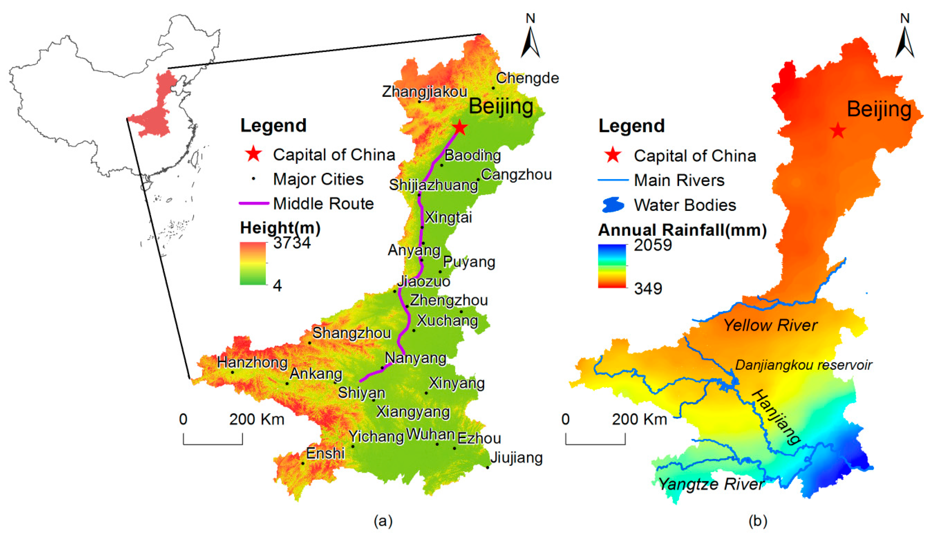
2.1. Brief Introduction to the Middle Route of the SNWDP

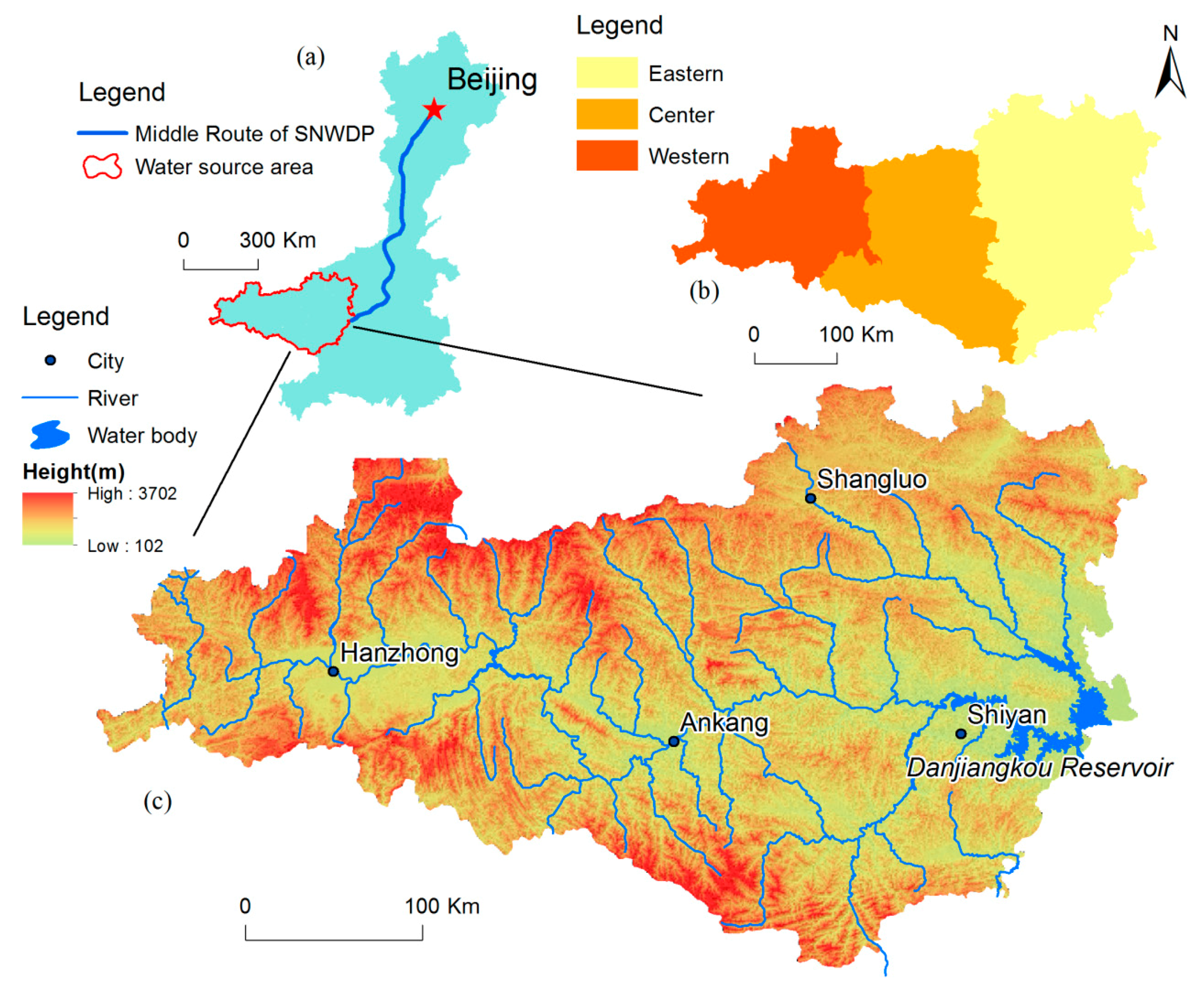
China has a large amount of water resources, but the per capita water resources is only a quarter of the world average, and the distribution is extremely uneven in time and space [36]. The water resources shortage has become a pivotal factor that restrict the sustainable development of social economy in some areas of China [37]. In China, the SNWDP is a strategic project to solve the uneven distribution of water resources and promote the coordinated development of the regions. The SNWDP includes three routes: the eastern, middle, and western. The middle route of the SNWDP diverts water from Danjiangkou Reservoir to North China (including the capital of China, Beijing) by heightening the Danjiangkou Dam. The total length of the main canal is approximately 1420 km (Figure 1). The total investment is about 92 billion yuan.

The construction of the middle route of the SNWDP started in January 2003 and formally completed in December 2014. The annual water amount transferred from the Hanjiang River Basin to North China is about 13 billion cubic meters. Solving the problem of urban water shortage in North China, including Beijing and Tianjin, is strategically significant—it also eases the contradiction between urban occupancy ecological and agricultural water consumption [38]. The ecological and environmental safety of the WSA is the key to the sustainability and stability of the middle route of the SNWDP. Since the construction of the middle route of the SNWDP, the ecological and environmental security of WSA has attracted the attention of all sectors of society, including the state, local governments, and scholars [39]. However, due to the large population, complex topography, and high land use intensity, the WSA of the middle route of the SNWDP is still experiencing environmental risks such as soil erosion, NPS pollution, and water eutrophication. According to reports, the Danjiangkou Reservoir has been in the middle nutrition state for a long time [40]. The economy of the WSA of the middle route of the SNWDP is dominated by primary industry, and the rural population accounts for more than 60% of the total population. Eutrophication caused by NPS pollution plays an important role in the water quality, the sustainable development of the WSA, and the safety of the middle route of the SNWDP.

2.2. Study Area

Our study area is the WSA of the middle route of the SNWDP, between the Qinba Mountains, where the North–South transition and the East–West alternation occur in China. It is located in the upper reaches of the Hanjiang River, which is the largest tributary of the Yangtze River. Additionally, the Hanjiang River runs from west to east across the study area. The Danjiang River occupies the northeast of the study area and flows into the Hanjiang River from the northwest to the southeast. Except for the Hanzhong Basin, the other landforms in the study area are mainly middle and low mountains and hills, with characteristic alternating valleys and basins. The study area belongs to the north subtropical monsoon zone with warm semi-humid climate, distinct seasons, uneven precipitation distribution, and obvious stereoscopic weather. The annual mean temperature of the study area is 13.7 °C. The annual mean precipitation is about 880 mm (range from 700–1200 mm). The time distribution of precipitation in the study area is uneven: 80% of the annual precipitation from May to October, and most of the rain occurs as torrential rain. In 2015, the total population of the study area was about 13.37 million, the cultivated land area was about 24,000 km², and the gross domestic product (GDP) was about 423.90 billion yuan. The study area is located in the concentrated poverty-stricken areas of Qinba Mountains. There were 2.57 million poor people and 18 poverty-stricken counties. Compared with surrounding regions, the economic and social development level in the research area is relatively low.

The complex topography, uneven distribution of rainfall, and strong demand for social and economic development lead to a great risk of NPS pollution in the research area. The ecological security of our study area has an important strategic position for the middle route of the SNWDP. It is necessary and urgent to carry out research on NPS pollution in the study area.

According to "The 13th Five-Year Plan for Control of Water Pollution and Soil and Water Conservation in Danjiangkou Reservoir Area and Upper Reaches" [41], the administrative divisions of the WSA cover 46 counties in 14 cities in Shaanxi, Hubei, and Henan provinces, as well as some towns and townships of Wanyuan in Sichuan province, Chengkou County in Chongqing, and Liangdang County in Gansu Province, ranging from 31°31′ to 34°25′ N and 105°31′ to 112°02′ E. Considering the integrity of the administrative unit, the following adjustments were made on the basis of the above planning scope: (1) some townships (non-complete county area) of Wanyuan City, Chengkou County of Chongqing, and Liangdang County of Gansu province were excluded; (2) Xichuan County of Henan province and Fangxian of Hubei province were added; and (3) merging urban districts into urban areas. After adjustments, our study area covers 40 counties (districts) with a total area of about 108,736 km² (Figure 2).

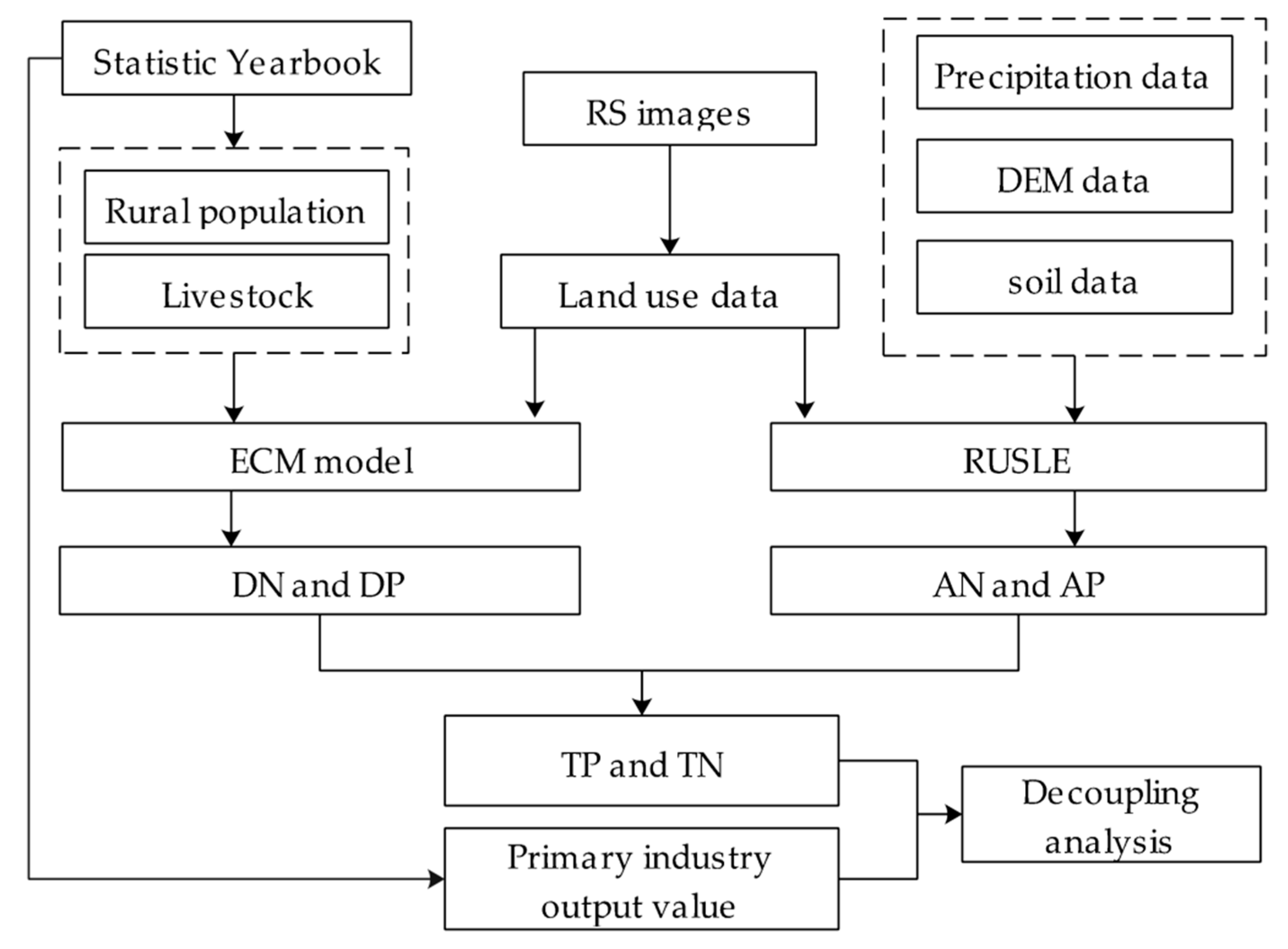
3. Materials and Methods

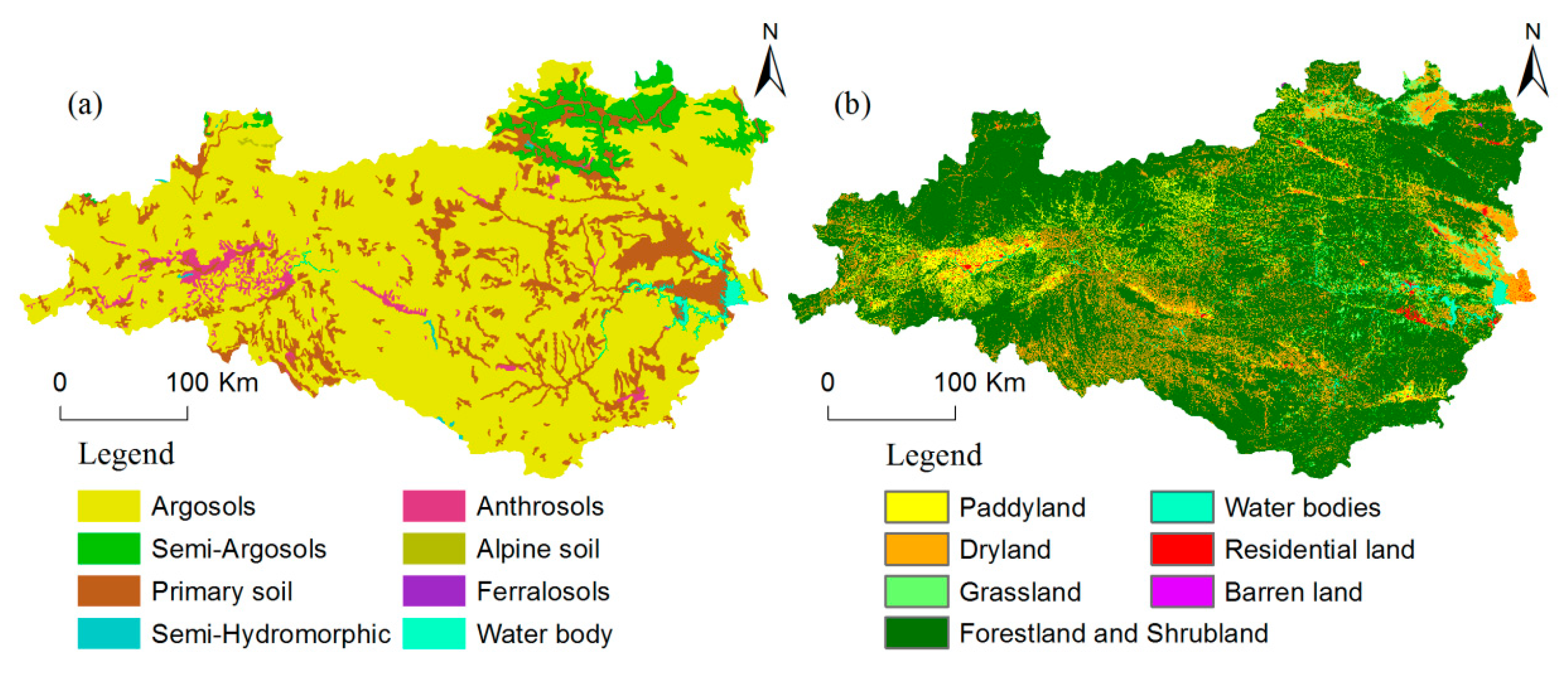
3.1. Data Source

The following datasets were used in this study: (1) Land-use datasets for 2000, 2005, 2010, and 2015 were interpreted from Landsat images. The resolution of the images was 30m, and their imaging time was ± 2 years for each year. The images were obtained from Geospatial Data Cloud, Computer Network Information Centre, Chinese Academy of Sciences [42], and interpreted using Environment for Visualizing Images (ENVI) software (version 4.8, Harris Corporation, Melbourne, FL, USA, 2010) (Figure 3b). (2) Historical rural population, livestock used in ECM, and PIOV used for decoupling analysis were obtained from the Statistical Yearbook of each city. (3) Digital elevation model (DEM) with a resolution of 30 m was also downloaded from Geospatial Data Cloud [42]. (4) Historical precipitation data sets (from 2000 to 2015) were obtained from Earth System Research Laboratory, National Oceanic and Atmospheric Administration, U.S. Department of Commerce [43,44]. (5) Soil database with properties of nitrogen content and phosphorus content was obtained from the 1:1,000,000 soil database provided by the Nanjing Soil Research Institute, Chinese Academy of Sciences (Figure 3a). Using ArcGIS software package (version 10.2, Environmental Systems Research Institute, Redlands, CA, USA, 2013), all the spatial datasets mentioned above were projected into a same projection (Albers Equal Area Conic) and the resolution was set to 30 m.

3.2. Estimation of NPS Pollutants Amounts

Dissolved NPS pollutants are commonly delivered by rainfall to waters and mainly generated by agriculture practices, such as land-use, rural population living, and livestock breeding. The values can be estimated using the export coefficient model (ECM). The adsorbed NPS pollutants are mainly controlled by soil erosion and they can be estimated using the Revised Universal Soil Loss Equation (RUSLE) [12].

$$E_{NPS}=E_{dis}+E_{ad}$$

(1)

where $E_{NPS}$ is the total NPS pollution load (t/year), $E_{dis}$ and $E_{ad}$ represent loads of the dissolved NPS pollution and adsorbed NPS pollution, respectively (t/year).

3.2.1. Export Coefficient Model

Dissolved nitrogen and phosphorus (DN and DP, respectively) loads could be calculated using the export coefficient model (ECM). The ECM improved by Johnes in 1996 was used in this study to estimate dissolved NPS pollution loads [21]. Taking the land-use classifications into consideration, the output coefficients of different pollution sources were determined using the ECM model on the basis of the rural population and livestock and the discharge and treatment of NPS pollutants [45]. The general expression of the model is

$$E_{dis}={\displaystyle \sum }_{i=1}^n{\displaystyle \sum }_{j=1}^m{E}_{ij}{A}_{ij}+P_i$$

(2)

where $E_{dis}$ is the dissolved NPS pollution load (t/year); m is the type of pollutant, which is dissolved nitrogen (DN) and dissolved phosphorus (DP); $E_{ij}$ is the export coefficient for pollution source j (kg/km²·year for land use or kg/ca·year for human or livestock discharge) in unit i; $A_{ij}$ represents the area of land-use type or the number of population (rural life) or livestock in unit i; and $P_i$ indicates the pollution input from rainfall in unit i. Due to the lack of data, the input nutrient pollution from rainfall was omitted in this study.

There are two methods to obtain export coefficient $E_{ij}$: field monitoring and literature review. Because field monitoring is expensive and time consuming, we referenced research results in neighboring regions from other scholars to determine the export coefficients (

Table 1. Export coefficients of different NPS pollution sources

NPS Pollution Sources	Export Coefficients
	DN	DP
Paddy field (kg/(km2 × year))	2625	182
Dry land (kg/(km2 × year))	1921	79
Forestland (kg/(km2 × year))	655	18
Shrubland (kg/(km2 × year))	1032	23
Grassland(kg/(km2 × year))	1135	38
Residential land(kg/(km2 × year))	636	36
Barren land(kg/(km2 × year))	1121	64
Rural population (kg/((ca × 104) × year))	19,547	2142
Cattle (kg/((ca × 104) × year))	113,715	2179
Pigs (kg/((ca × 104) × year))	26,667	1417
Goats (kg/((ca × 104) × year))	15,134	450
Poultry (kg/((ca × 104) × year))	459	54

) [45,46]. Using the results of previous studies will bring uncertainties to our results. However, we focused more on the change tendency of NPS pollution, not the absolute values. This approach can achieve this aim.

3.2.2. RUSLE Model

Adsorbed pollutants are transported by soil erosion. The amount of adsorbed nitrogen (AN) and phosphorus (AP) can be assessed using the equation [12]

$$E_{ad}=\lambda \times ({\displaystyle \sum }_{i=1}^{n}Rusl{e}_i\times S_i\times C_j\times \mathsf{\beta })$$

(3)

where $E_{ad}$ is the adsorbed NPS pollution load (t/year), and $\lambda$ is a coefficient that affects the AP and AN loads drained into the lake. According to previous results, the value of $\lambda$ was reported as 0.28 [47]. $Rusl{e}_i$ represents the mean soil loss from land use type i in Equation (4), $S_i$ is the area of land use type i, and $C_j$ is the background content of nitrogen or phosphorus in the soil (%), which can be available in the 1:1,000,000 soil database. The $\mathsf{\beta }$ of nitrogen or phosphorus are 1.35 and 1.28, respectively, according to the previous literature [48].

Different scholars have assessed soil erosion in a variety of ways, by using the Instituto Nacional para la Conservación de la Naturaleza (ICONA) model [49] and RUSLE model [50,51,52]. Sediment dynamics at the catchment scale depend primarily on climate (especially the rain intensity), soil, and vegetation characteristics, and factitious factors such as agricultural activities or dam construction and operation [53].

The sum of annual soil loss for unit i is calculated by the equation

$$Rusl{e}_i=R_i\times K_i\times L{S}_i\times C_i\times P_i$$

(4)

where $Rusl{e}_i$ is the amount of annual soil loss for unit i (t/(ha × year)); $R_i$ denotes the precipitation erosivity element; $L{S}_i$ is the slope length-gradient element, come a combination of the slope steepness factor and slope length factor; $C_i$ is the crop-management practice factor; and $P_i$ is the conservation support practice factor. The $C_i$, and $P_i$ factors referenced results of other scholars [54].

The descriptions and sources of the inputs needed in the RUSLE model in our study were as follows. All input GIS maps or rasters for accurate results were conducted in the same projection and linear meter units.

(1) Rainfall erosivity index (R): A GIS raster dataset with an erosivity index value for each unit, reflecting climate properties. The R factor is the annual long-term mean of the product of events of rainfall kinetic energy, which quantifies the effect of rainfall and associated runoff impact [26,55]. In this study, we refer to Wischmeier’s results as [56]

$$R={\displaystyle \sum }_{i=1}^{12}1.735\times {10}^{\left(1.5\times {\log }_{10}\left(\frac{P_i^2}{P}\right)-0.08188\right)}$$

(5)

where R represents the rainfall erosivity factor ((MJ × mm)/ha × h ×⋅year), $P_i$ represents monthly average rainfall (mm), and P represents annual rainfall (mm).

(2) Soil erodibility (K): K is a GIS raster dataset with a soil erodibility value for each unit. K is a measurement index of the sensitivity susceptibility of soil particles to detachment and transport though rainfall and runoff. The dataset was mainly cited from previous results that focused on central China [57]. The K values for different soil types are listed in

Table 2. Soil erodibility values from previous studies.

Soil Types	K-Value	Soil Types	K-Value
Yellow-brown soils	0.225	Skeletol soils	0.190
Yellow-cinnamon soils	0.245	Lime concretion black soils	0.262
Brown earths	0.273	Mountain meadow soils	0.254
Dark-brown earths	0.281	Fluvo-aquic soils	0.292
Cinnamon soils	0.340	Paddy soils	0.253
Red clay soils	0.310	Dark felty soils	0.321
Purplish soils	0.241	Yellow earths	0.248
Litho soils	0.255	–	–

.

(3) Topographic factor (LS): LS is calculated by multiplying slope length factor (L) and slope steepness factor (S). In this study, we referenced the following algorithms, which were previously developed to calculate the LS factor [58,59,60]

$$\mathrm{L}={\left(\mathsf{\lambda }/22.13\right)}^u$$

(6)

$$u=n/\left(1+n\right)$$

(7)

$$n=\left(\sin \mathsf{\theta }/0.0896\right)/[3.0{\left(\sin \mathsf{\theta }\right)}^{0.8}+0.56]$$

(8)

where λ represents the horizontal projection (unit: m), 22.13 is the RUSLE unit plot length (unit: m), and $\mathsf{\theta }$ is slope degree.

The S factor is calculated according to the angle using the equations [59]

$$\mathrm{S}=10.8\sin \mathsf{\theta }+0.03\hspace{1em}\hspace{1em}\mathsf{\theta }<5°$$

$$\mathrm{S}=16.8\sin \mathsf{\theta }-0.5\hspace{1em}\hspace{1em}5°\le \mathsf{\theta }<10°$$

(9)

$$\mathrm{S}=21.91\sin \mathsf{\theta }-0.96\hspace{1em}\hspace{1em}\mathsf{\theta }\ge 10°$$

(4) Crop-management practice factor (C): C factor is a floating point value between 0 and 1.

(5) Conservation support practice factor (P): P is the support practice factor for the RUSLE model, and a floating point value is between 0 and 1.

Because the Three Gorges area is close to the study area and they have many similarities, the C value and P value were directly obtained from Liu’s [54] research results in the Three Gorges Reservoir area.

3.3. Decoupling Analysis

The following mathematical expression is used to calculate decoupling index (DI)

DI = ∆E_NPS/∆V_PIOV = (E_NPSi/E_NPSi−1 − 1)/(∆V_PIOVi/∆V_PIOVi-1 − 1)

(10)

where ∆E_NPS and ∆V_PIOV are the change in the rate of NPS pollution loads (t/year) and PIOV, respectively; E_NPSi and V_PIOVi represent the pollution loads and PIOV at the last phase, respectively; and E_NPSi-1 and V_PIOVi-1 represent the corresponding value in the base period. There are six possible combinations of ∆E_NPS and ∆V_PIOV , and the different decoupling degrees are described in

Table 3. Classification and criteria for decoupling

Decoupling Degrees	Relationship between PIOV and Total NPS Pollution Load
Strong decoupling (SD)	∆ENPS ≤ 0, ∆VPIO > 0, DI < 0
Recessive coupling (RC)	∆ENPS ≥ 0, ∆VPIO < 0, DI ≤ 0
Weak decoupling (WD)	∆ENPS > 0, ∆VPIO > 0, 0 < DI < 1
Expansive coupling (EC)	∆ENPS > 0, ∆VPIO > 0, DI ≥ 1
Weak coupling (WC)	∆ENPS < 0, ∆VPIO < 0, 0 ≤ DI < 1
Recessive coupling (RC)	∆ENPS < 0, ∆VPIO < 0, DI ≥ 1

[29]. Figure 4 shows the basic data required for this study, as well as the intermediate calculation process and results.

4. Results

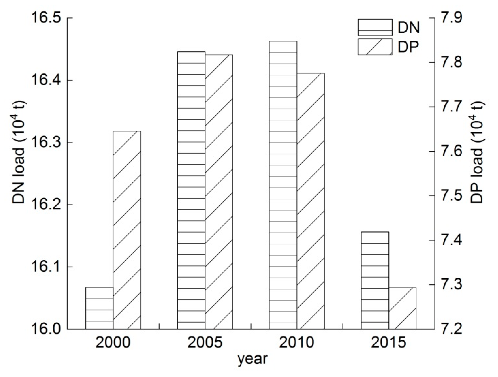
4.1. DN and DP Estimation

4.1.1. Temporal Variations in DN and DP

The estimated results of DN and DP loads for 2000–2015 are shown in Figure 5.

It can be seen in Figure 5 that the amount of DN and DP estimation fluctuated in different patterns. The annual amount of DN load enlarged before 2010 but declined after 2010 with a peak of 164,625.51 t/year. The DN load in 2015 increased slightly compared with 2000, with an increase of 0.55%. For DP load, the inflection point from increase to decline was 2005 with a peak value of 7293.33 t/year. In 2015, the DP load in the study area was 7293.33 t/year, with a slight decrease of 4.60% compared with 2000. The analysis above shows that the DN loads increased slightly over the 15-year period, but the growth trend was restrained after 2010. The DP load decreased significantly during the study period, and the decreasing tendency was significant after 2005.

Over the past 15 years, significant changes have taken place in land use in the study area, as shown in

Table 4. Land use area in different years.

Land Use Types	2000	2005	2010	2015
Barren land (km2)	10.80	10.80	11.76	24.27
Dry land (km2)	15,766.81	15,497.21	15,473.18	15,440.34
Grassland (km2)	4118.02	4135.09	4103.15	4057.47
Paddy field (km2)	9060.50	9004.65	8889.55	8785.12
Residential land (km2)	566.37	628.93	765.85	995.24
Shrubland (km2)	51,529.33	51,712.11	51,824.92	51,729.63
Waterbody (km2)	976.84	1037.55	1110.10	1189.12
Woodland (km2)	26,707.76	26,710.09	26,557.95	26,515.25

.

As can be seen from Table 4, the area of cultivated land (including dry land and paddy land) in the study area has decreased obviously. Cultivated land made the largest contribution to DN and DP loads and account for 32.75% and 37.43%, of the total amount of dissolved NPS pollution, for multi-year average. Compared with 2000, DN and DP loads caused by cultivated land decreased by 1350.01 t/year and 75.91 t/year in 2015, with a reduction of 2.5% and 2.62%, respectively. The decrease of cultivated land area was beneficial to reduce DN and DP loads. The area of residential land and barren land were increasing significantly. Compared with 2000, DN and DP loads caused by residential land and barren land increased by 77.32% and 76.83% in 2015, respectively. Although the multi-year average ratio of DN and DP loads caused by residential land and barren land to the total amount of dissolved NPS pollution were 0.30% and 0.36%, the increase of residential and barren land could increase the risk of NPS pollution.

In addition, due to the impacts of immigration and urbanization, the rural population in the study area has decreased significantly over the past 15 years. In 2000, 2005, 2010, and 2015, the rural population was 11.82 million, 11.76 million, 11.39 million and 8.61 million, respectively. Compared with 2000, the rural population decreased by 27.16% in 2015, and the DN and DP loads caused by rural life decreased by 6272.19 t/year and 687.32 t/year respectively. The decrease of rural population can reduce the loads of DN and DP. It is worth noting that in the past 15 years, the total amount of livestock in the study area has been increasing. Compared with 2000, the amount of livestock increased by 105.47% in 2015, and the DN and DP loads caused by livestock increased by 8212.73 t/year and 396.48 t/year respectively. The increase of livestock would increase the risk of NPS pollution.

The variation of DN and DP loads in the study area was the result of the interaction of the parameters mentioned above. The changes in these parameters may be due to the following reasons: In 2006, the State Council of China approved and implemented “The Danjiangkou Reservoir Area and Upper Reaches Water Pollution Prevention and Control and Soil and Water Conservation Plan”, which began to comprehensively prevent and control the environmental pollution in the study areas. As important parts of the above plan, the Small Watershed Comprehensive Management Project, the Conversion of Farmland to Forestry Project, and the Ecological Migration Project have been implemented. The implementation of these projects may has played a positive role in the control of NPS pollution in the study area.

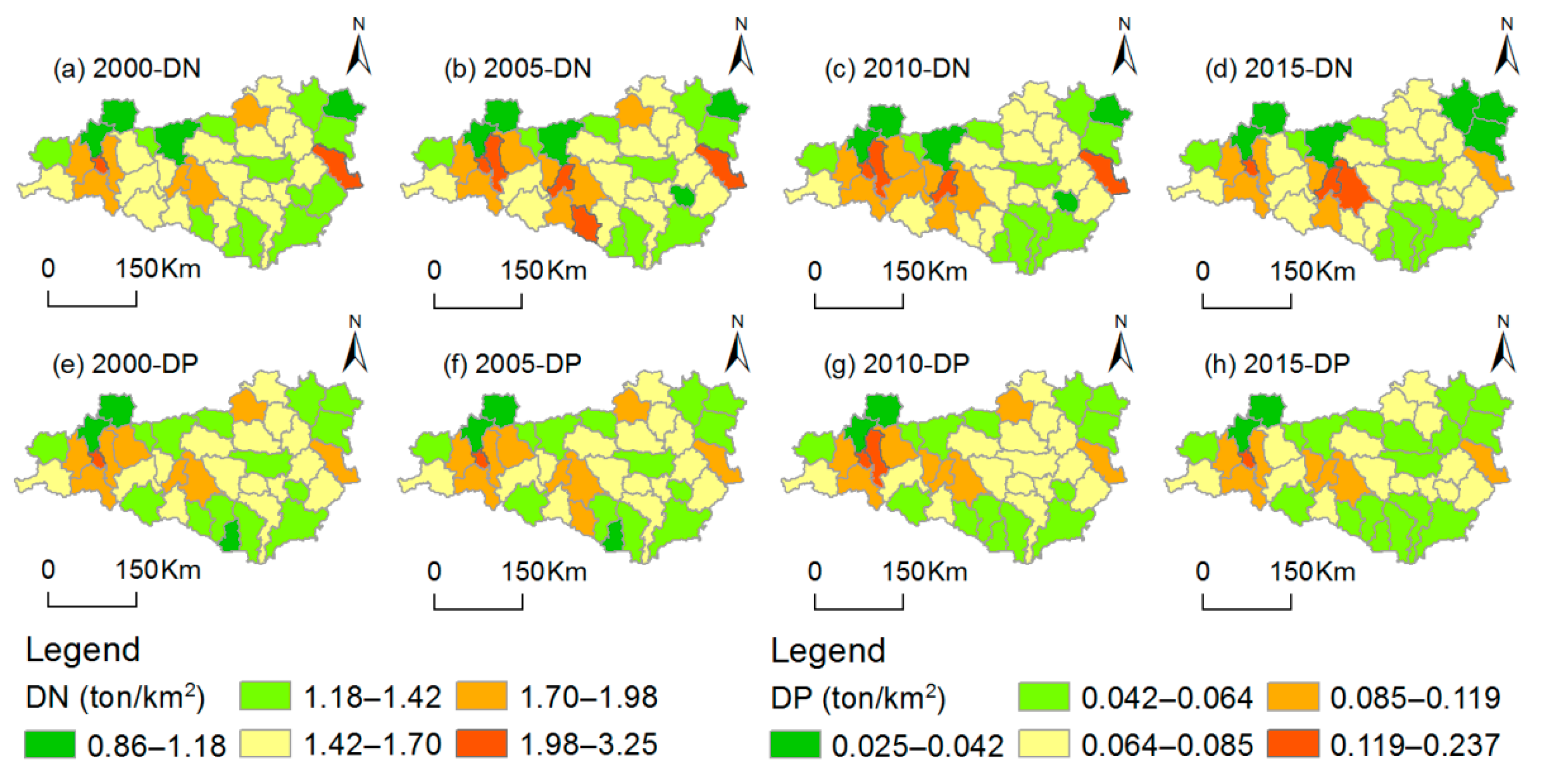
4.1.2. Spatial Variations in DN and DP

The annual load intensities of DN and DP in different counties during the simulated years are shown in Figure 6.

The spatial distributions of DN and DP loads intensities observed over the study years exhibited a similar pattern and did not change much. Counties with high DN and DP loads intensity were mainly concentrated in two regions in the west: Hanzhoung Basin and Ankang Basin. This may be due to the large amount of cultivated land and the high density of rural population in these two basins. According to the Statistical Yearbooks, in 2015, pure nitrogen and phosphorus fertilizer intensity of cultivated land in Hanzhong Basin and Ankang Basin were about 1.84 t/ha and 0.73 t/ha, respectively. While the average values in Hubei, Henan, and Shaanxi were about 0.26 t/ha and 0.13 t/ha, respectively, in the same year. Heavy fertilizer use intensity might be the cause of high estimated results of DN and DP in Hanzhong Basin and Ankang Basin [61]. Figure 6e–h shows that the number of counties with high DP load intensity decreased over the study period. Notably, Xichuan County, which is located in the east of the study area, had relatively high DN and DP load intensities. Xichuan had a large amount of cultivated land, accounting for 42.77% of its total area in 2015. Although the rural population of Xichuan decreased from 640,000 in 2000 to 456,000 in 2015 due to emigration and urbanization, its total rural population was still larger than that of other counties. The large rural population led to intensive utilization of cultivated land, which might be the cause of high intensity NPS pollution load.

From the above analysis, we concluded that the dissolved NPS pollution load intensities in the western region were relatively high and need to be given priority. Xichuan County also needs to be an area of focus due to its high dissolved NPS pollution load intensity.

Since the county is the basic unit of administration in China, the analysis of the total DN and DP loads of different counties can provide more information for the implementation of preventive operational measures. The spatial pattern evolution of DN and DP loads in different counties are shown in Figure 7. Over the 15-year period, the spatial distribution pattern of counties with high DN load did not change much. Counties with high DN load were primarily distributed in the eastern and center regions, and gradually converged to the eastern part. Counties with high DP load were mainly concentrated in the eastern and western regions, and continuously gathered in the eastern region. The number of counties with high DP load decreased from eight to four from 2000 to 2015. Although the intensity of dissolved pollution load in most eastern counties was relatively low compared to the western counties, the total load of these counties was consistently high because of their large area. In the future, more attention also should be given to the eastern counties to prevent and control the dissolved NPS pollution.

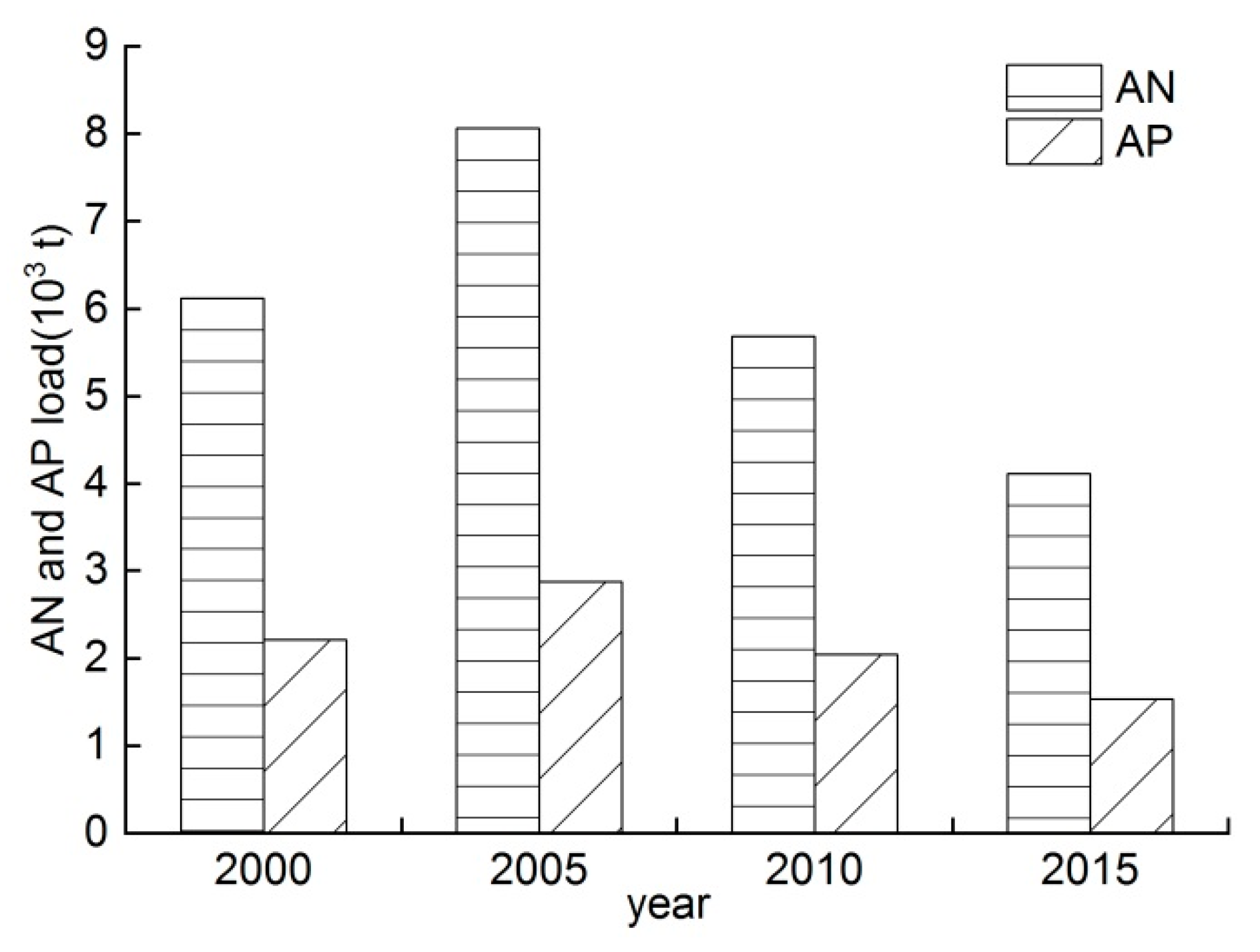
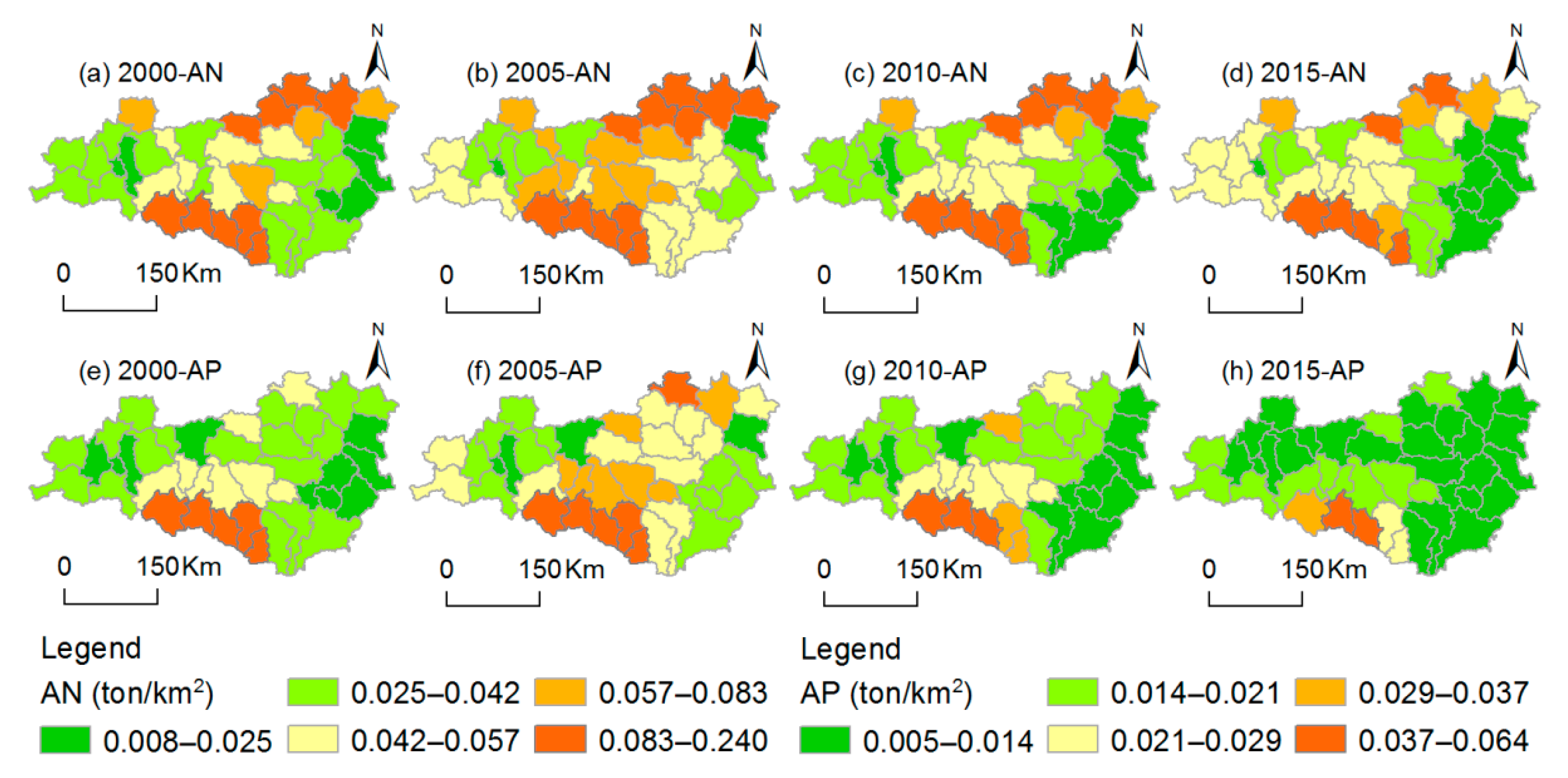
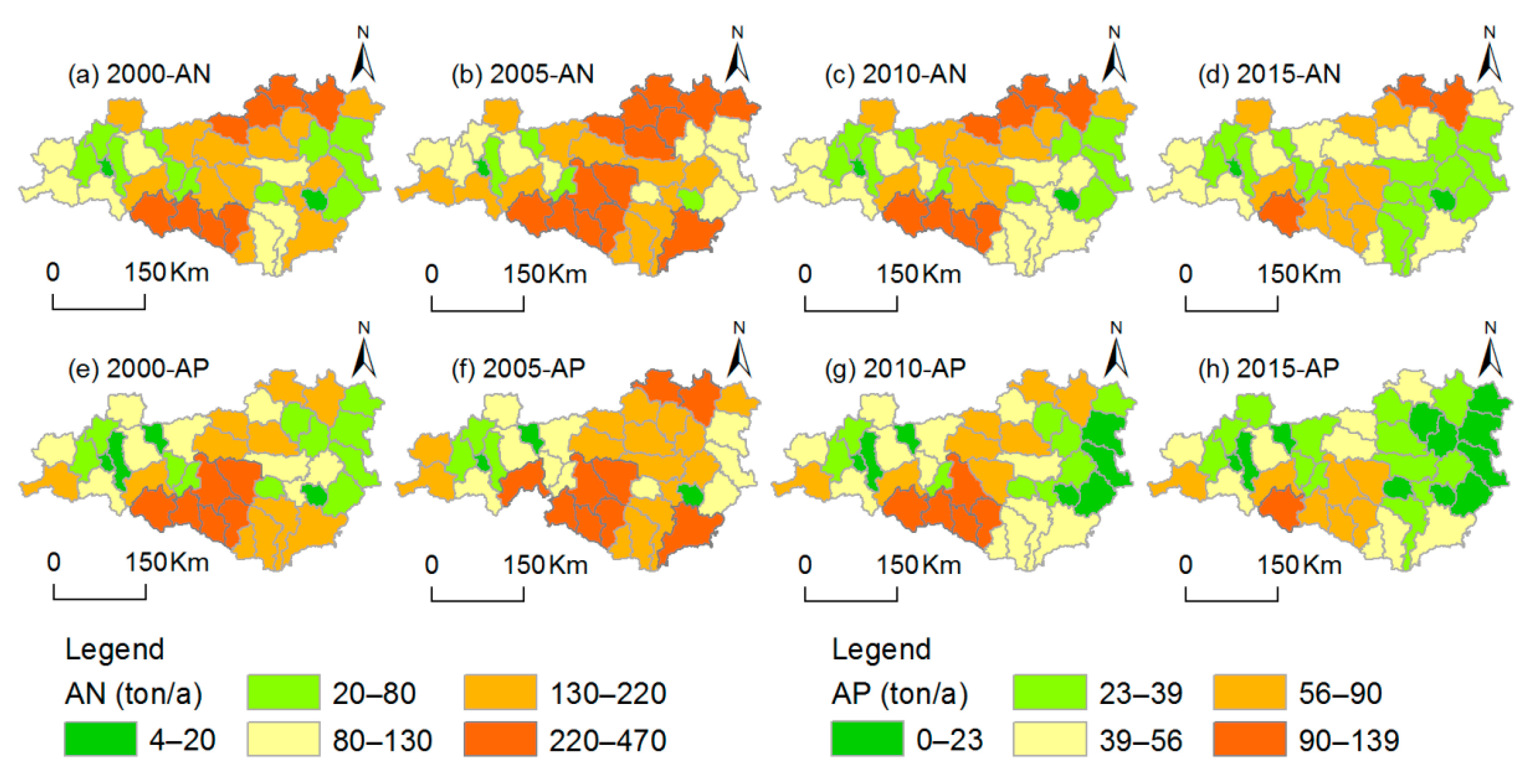
4.2. AN and AP Estimation

4.2.1. Temporal Variations in AN and AP

The estimated results in AN and AP loads are shown in Figure 8.

From Figure 8, the estimated results of AN and AP loads fluctuated in similar patterns. The annual loads of AN and AP increased obviously before 2005 and then decreased after 2005, with peaks at 8062.75 t/year and 2871.12 t/year, respectively. Compared with 2000, the AN and AP loads in 2015 significantly decreased by 32.72% and 30.81%, respectively.

The loads of AN and AP are mainly controlled by the intensity of soil erosion. According to RUSLE (Equation (4)), the average soil erosion intensity in 2000, 2005, 2010, and 2015 were 119.13 t/(ha × year), 154.57 t/(ha × year), 109.79 (t/(ha × year) and 82.61 t/(ha × year), respectively. In the past 15 years, the intensity of soil erosion in the study area decreased significantly, which was the main reason for the decrease of AN and AP estimation. The above phenomenon can be explained as follows. Since 2005, the construction of the middle route of the SNWDP has been in a critical period. In order to guarantee the water quality, in October 2007, the Chinese governments started the “Water and Soil Conservation Project in the WAS of the Middle Route of SNWDP” [62]. The government has paid much attention to this area and a series of projects have been formulated and implemented, such as the closing hills for afforestation, the conversion of cropland to forest or grassland, the land consolidation, and the Small Watershed Comprehensive Management Project. The area of cultivated land (including dry land and paddy land) in the study area has decreased obviously. Compared with 2000, the cultivated land area decreased by 2.42% in 2015. At the same time, the area of forests (including woodland and shrubbery) increased by 0.99%, and the area of water increased by 21.73%. Under the combined effect of the above changes, the soil erosion has been effectively restrained. Notably, the rainfall intensity in 2010 and 2015 was lower than usual, which might have contributed to the decline in AN and AP loads as well. Under the combined effect of the above factors, AN and AP loads decreased significantly.

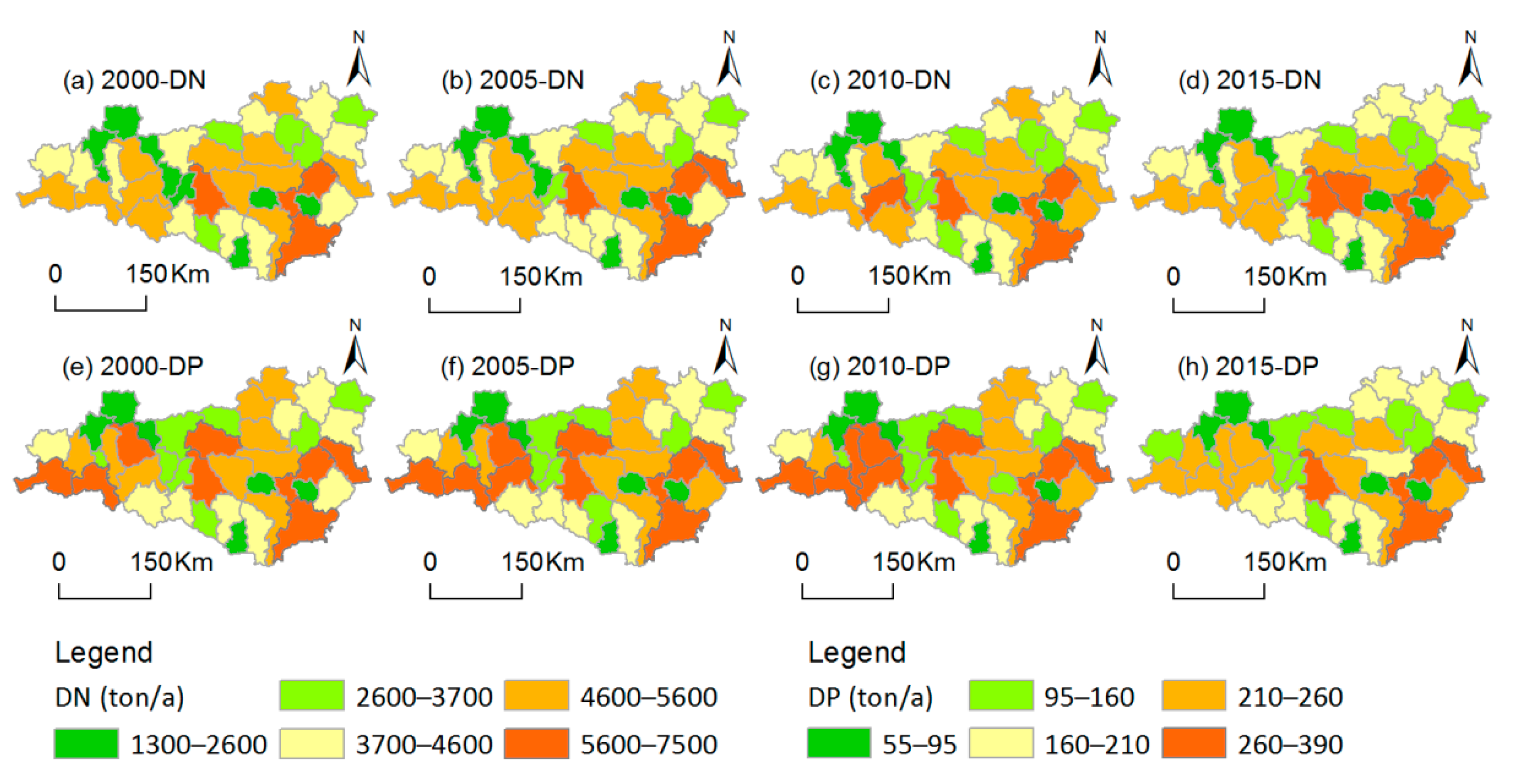
4.2.2. Spatial Variations in AN and AP

The intensities of the AN and AP loads in different counties during the observed years are shown in Figure 9.

Compared to the dissolved pollutants, the load intensities of the adsorbed pollutants indicated a very different spatial distribution pattern. Counties with high AN load intensity were primarily located in the southern and northern regions of the study area. The number of counties with high AN load intensity decreased significantly, and the decrease in the northern region was more obvious. Counties with high AP load intensity were mainly concentrated in the southern region, the number of which decreased significantly over the 15-year period. The northern and southern regions have steep topography and relatively low vegetation coverage, which resulted in strong soil erosion. Since adsorbed pollutions are mainly controlled by soil erosion, strong soil erosion might be the main cause of high AN and AP load intensity. As for AN load, the soil type in the northern part is mainly semi-argosols, which contains relatively high amounts of background N. This may be also an important reason for the heavy AN load intensity in the northern region. In the future, measures for soil and water conservation in the southern and northern mountainous areas should be strengthened, such as the closing hills for afforestation and returning farmland to forests. The sensitive counties mentioned above should receive a spatially targeted approach to reducing adsorbed pollution.

From the spatial variations in total AN and AP loads of different counties (Figure 10), we learned that the spatial distribution of counties with high AN and AP loads has good consistency with the spatial distribution of intensities. Over the 15-year period, the total AN and AP loads in most counties showed a decreasing trend. We must focus on the fact that the total loads of AN and AP in southern counties were still relatively large, and these counties should be given priority support in terms of funds and policies.

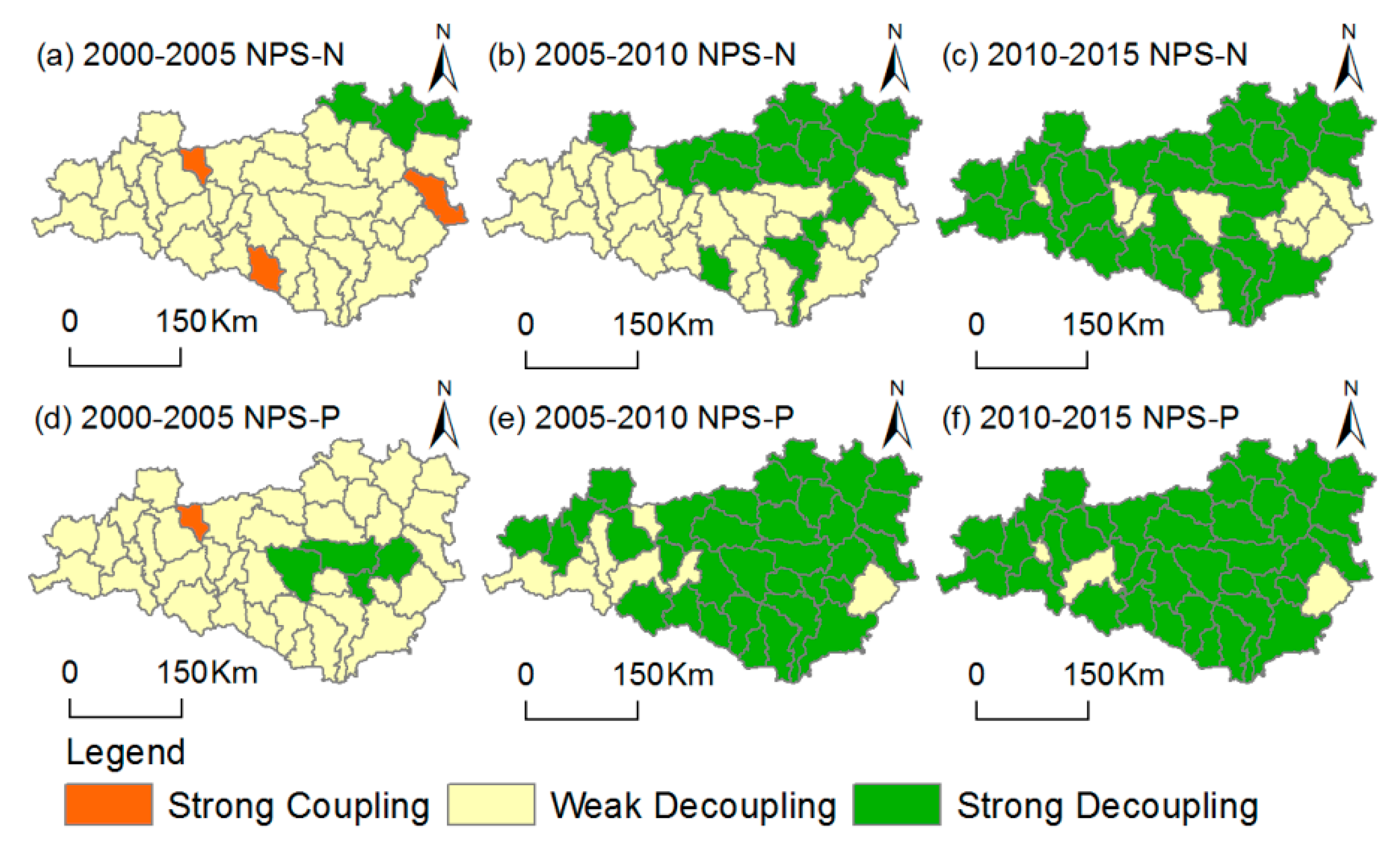
4.3. Decoupling NPS Pollution from PIOV

The decoupling states NPS pollution from PIOV in 2000, 2005, 2010, and 2015 in the study area are shown in

Table 5. Results of decoupling NPS pollution from PIOV

Year	Growth Rate (%)			DI		Degrees of Decoupling/Coupling
	PIOV	NPS-N	NPS-P	NPS-N	NPS-P	NPS-N	NPS-P
2000–2005	53.07	3.43	8.43	0.06	0.16	WD	WD
2005–2010	112.51	−1.28	−8.12	−0.01	−0.07	SD	SD
2010–2015	62.78	−2.72	−10.15	−0.04	−0.16	SD	SD

Note: PIOV, DI, WD, and SD are the primary industries output value, the decoupling index, the weak decoupling, and the strong decoupling, respectively.

. From 2000 to 2005, the growth rate of PIOV was 53.07%, and the growth rates of NPS-N and NPS-P estimation were 3.42% and 8.43%, respectively. The growth rate of PIOV was much larger than that of NPS pollution, which resulted in a weak decoupling (WD) relationship between NPS pollutants and PIOV. From 2005 to 2010, the growth rate of PIOV increased to 112.51%, while the growth rate of NPS-N and NPS-P estimation were −1.28% and −8.12%, respectively, characterizing a strong decoupling (SD) relationship between them. After 2010, the increasing trend of PIOV did not change but the decreasing trend of NPS pollution was more obvious, which resulted in SD relationship between NPS pollution and PIOV.

Since the implementation of the construction of the middle route of the SNWDP, the governments have focused their attention on environmental protection and have implemented various methods to control NPS pollution while promoting the development of primary industry, such as accelerating the transformation and upgrading of agricultural structure and intensifying the efforts of rural environmental renovation. Under various efforts, the risk of NPS pollution caused by the development of primary industry has been gradually reduced.

The analysis of the decoupling situation in different counties can provide more scientific and technological supports for the formulation of relevant policies. The spatial pattern evolution of decoupling NPS pollution from PIOV in each county is shown in Figure 11.

From 2000 to 2005, the development of primary industries in most of counties showed WD from NPS pollutants. Three counties showed a strong coupling (SC) relationship between NPS-N and PIOV, and one county showed a SC relationship between NPS-P and PIOV. From 2005 to 2010, the development of primary industries in about half the counties was strongly decoupled from NPS-N pollution, and most counties were strongly decoupled from NPS-P pollution. From 2010 to 2015, most counties reached WD. Notably, there were some counties in the eastern counties (around Danjiangkou Reservoir) that were still in a WD state from NPS-N in 2015.

From 2000 to 2015, and especially after 2010, the development of primary industry in the study area gradually decoupled from NPS pollutants emissions. The above achievements may result from the environmental actions taken by the government, such as the strengthening of environmental protection, adjustment of agricultural structure, and the vigorous implementation of environmental renovation.

5. Discussion

5.1. Uncertainty of the Estimation Results

It must be noted that, since we used empirical models in this study, we have not been able to obtain long-term ground monitoring data in this area. The calculation results were only estimates of NPS pollution in this area. Some coefficients used in the models such as λ and β in the RUSLE model (Equation (3)), were cited directly from previous results, resulting in uncertainty in the estimated results. It is necessary to analyze the influence of the variation of these coefficients on the estimation results. With the estimated value in 2015 as an example, the estimated value of NPS-N and NPS-P would be reduced by 0.09% and 0.62%, respectively, for each decrease of the value of $\lambda$ by 0.01. When the ratios β of N and P in Equation (3) were reduced by 0.01, the estimated values of NPS-N and NPS-P would be reduced by 0.02% and 0.14%, respectively. From the analysis above, it can be seen that the coefficients have an important impact on the estimated results of the model, and the influences on the estimation results of NPS-P were greater than that of NPS-N. When using the model to estimate NPS pollution, special attention should be given to determine these coefficients scientifically to improve the preciseness of the model.

In addition, $E_{ij}$ used in the ECM model (Equation (2)) may have an impact on the estimated results. Collecting ground monitoring data with good quality to calibrate the coefficients used in the model are important, which will surely improve the simulation accuracy for environmental assessment—this deserves further research. Although there was uncertainty, the coefficients that we adopted were the previous results in adjacent regions with similar natural and social conditions, and our focus was more on the temporal changes and spatial comparisons of NPS pollution in the study area—the results of our research are of scientific value. In addition, the estimated results are also affected by input parameters, such as the number of rural population and livestock. Scenario analysis of these parameters is conducive to more detailed analysis of the uncertainty of model estimation results. The results of these scenario simulation can also help to put forward the preventive measures of NPS pollution.

5.2. Measures for Prevention

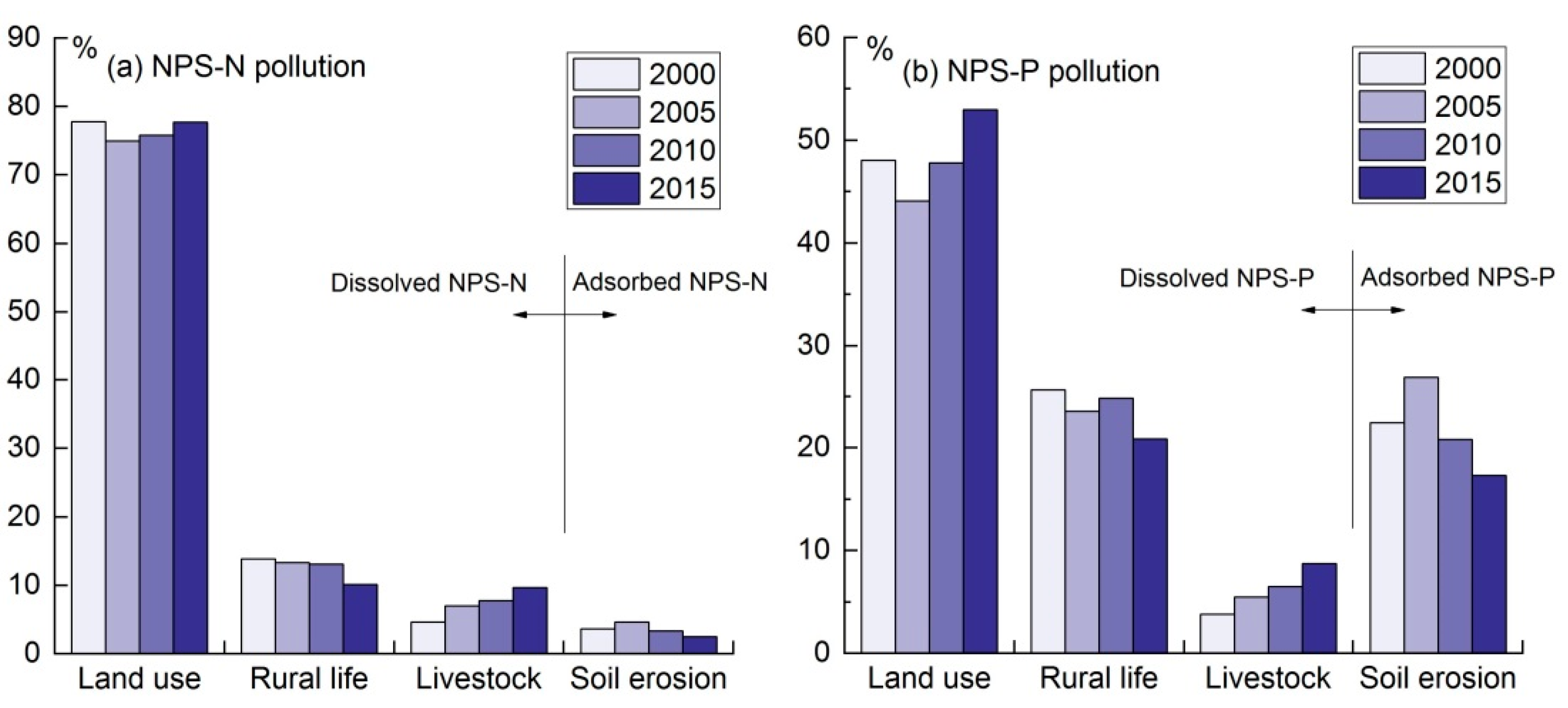
5.2.1. Composition Analysis of NPS Pollution

From the estimated results, the NPS-N load was much higher than the NPS-P load over the 15-year period. In comparing dissolved and adsorbed pollution, DN and DP loads controlled by land use, rural life, and livestock were much higher than AN and AP loads caused by soil erosion, accounting for 96.46% and 78.13% of the total NPS pollution, respectively, for multi-year average values. Dissolved pollution was the absolute source of NPS-N pollution in the study area (Figure 12).

In terms of the source of NPS pollutants (Figure 12), land use was the predominant contributor of NPS-N and NPS-P pollution, accounting for about 75% of NPS-N and 50% of NPS-P based on the average value over the study period. Therefore, it is necessary to adopt various measures to strengthen land use management and to moderately reduce the intensity of land use. Although the rural population in the study area has decreased by 27.16% in the past 15 years, and the intensity of soil erosion has also been effectively controlled, rural life and soil erosion were the other two important sources of NPS-P pollution in addition to land use, which also needs to be an area of focus. In the future, rural environmental infrastructure construction and soil and water conservation measures, such as land consolidation, can be strengthened to control NPS-P pollution. Notably, over 15 years, the amount of livestock increased by 105.47%. NPS pollutants caused by livestock grew significantly and have not been effectively controlled. Even though livestock was not the main source of NPS pollution, it also needs to be addressed immediately.

From the above analysis, the following conclusions could be drawn: (1) land use activities were the main source of NPS pollution in the study area; (2) rural life and soil erosion were important factors of NPS-P pollution; and (3) measures must be taken to curb the growth of NPS pollution caused by livestock.

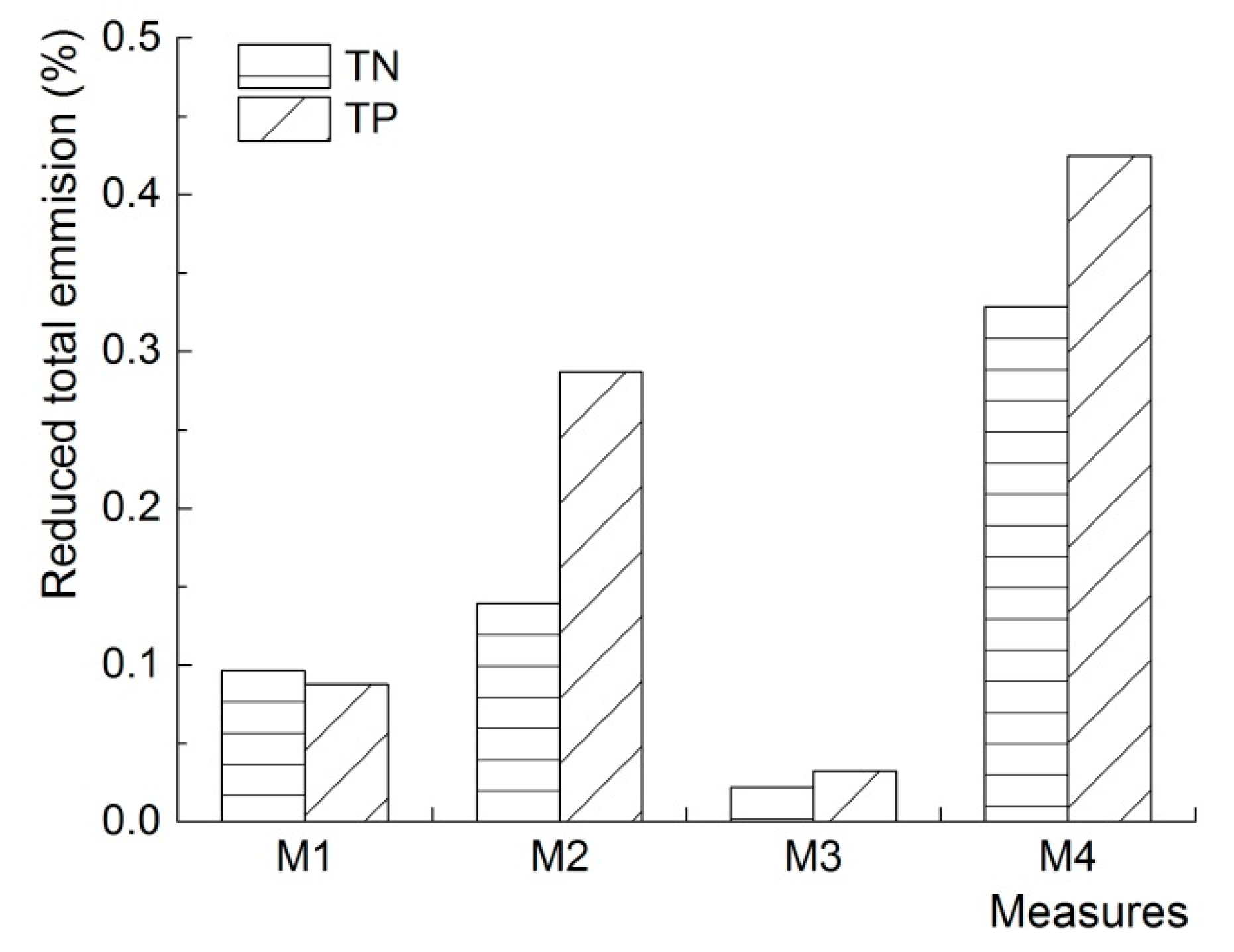
5.2.2. Measures for NPS Pollution Control

From the above analysis, it can be seen that the simulated values of NPS pollution load were controlled by land use, rural life, livestock breeding and soil erosion. Therefore, the measures to control NPS pollution can be considered from the above aspects. With the estimated value in 2015 as an example, we tried to find measures to reduce the emission of NPS pollution. Possible measures are as follows:

• Measure 1 (M1): Reducing the number of livestock.
• Measure 2 (M2): Reducing the rural population.
• Measure 3 (M3): Improving the capacity of waste treatment.
• Measure 4 (M4): Conversion of cropland to forest.

In order to compare and analyze the effects of different measures on NPS pollution emissions, the changes of estimated values of NPS pollution were evaluated for each 1% change of the given variable in different measures. The results are shown in Figure 13.

It can be seen in Figure 13 that the conversion of cropland to forestry (M4) has the greatest impact on the estimated value of NPS pollution emissions. When other conditions remain unchanged, the estimated value of NPS-N and NPS-P pollutant in 2015 would be reduced by 0.33% and 0.42%, respectively, while 1% of cultivated land was converted into woodland. The second is Measure 2 (M2). For every 1% reduction of the rural population, the estimated emissions of NPS-N and NPS-P pollutants will be reduced by 0.14% and 0.29%, respectively. Therefore, we should focus on the works of returning cropland to forest. If practical conditions are feasible, reducing the rural population is also an efficient means of decreasing the amount of NPS pollution.

Of course, the measures mentioned above can be carried out in a variety of combinations at the same time to lead to more sustainable management. It is worth pointing out that the cost of taking different measures varies. What measures or combinations of measures to take in the future needs to be determined according to cost estimates in different regions.

5.3. Comparison with Previous Studies

5.3.1. Previous Studies in Other Regions

Madjid Delkash et al. [22] found that the prediction accuracy of the SWAT model was higher than that of the ECM model after comparing the two models’ capacity to predict NPS pollution. At the same time, they pointed out that the predicted results of ECM on NPS-P were significantly affected by the coefficients, and the coefficients used in the ECM model should be various for different basins. The coefficients of the ECM model used in this paper were derived from previous results in adjacent regions with similar natural and social conditions—there were inherent uncertainties. However, the model has obvious advantages in analyzing the long-term variation and large-scale spatial contrast of NPS pollution. Collecting ground monitoring data and modifying model coefficients will be our future research direction. Daniel Ierodiaconou et al. [19] combined remote sensing data with the ECM model to study the changes of nitrogen and phosphorus loads in the Glenelg–Hopkins region in Australia over the past 22 years. The results showed that the ECM model is of great significance to the regions lacking long-term historical monitoring data. The situation in this study area is similar, so it is feasible and necessary to use the ECM model to estimate NPS pollution.

Scholars have also carried out relevant studies in other areas of China. Cheng et al. [63] studied the effects of different factors on NPS-P pollution in semi-arid areas of northern China by using the improved ECM model. They found that the rural population contributed the most to NPS phosphorus emission, while land use had the least impact, which was different from this study. The above situation shows that the same factor may differ greatly in the impact of NPS pollution in different areas, and it is necessary to conduct a specific analysis before employing control measures. Research by Zhang et al. [64] in the Three Gorges Reservoir Area showed that there was a close relationship between rural net income and NPS pollution. This paper analyzed the relationship between the PIOV and NPS pollution and analyzed the temporal and spatial changes of this relationship in different counties. Our research was more detailed than Zhang’s. Yang et al. [29] found that the relationship between grain production and NPS pollution in Heilongjiang land consolidation area was weak decoupling for most of the years. NPS pollution is not only controlled by grain production, but also rural population and livestock, etc. PIOV is more representative of the intensity of agricultural activities. This paper analyzed the relationship between NPS pollution and PIOV, which is a meaningful complement to Yang’s research.

The existing literature is quite abundant, and it is difficult to make a complete description. Some other results which provide important references for this study have been cited elsewhere in this paper.

5.3.2. Previous Studies in the Same Area

Previous studies estimated the NPS-N and NPS-P loads of the study area. Han. et al. [45] calculated the NPS-N load based on the ECM for a typical watershed in this region. However, they did not estimate the NPS-P pollution and did not consider the adsorbed NPS pollution, which may have resulted in an underestimation of NPS pollutants. The load intensity of NPS-N load in this study was 1.48 t/km² in 2015, which was much lower than Han’s result of 2.96 t/km² in 2014. The main reason was that Han’s research only focused on a typical small watershed in our study area, where the total agricultural population, cultivated land, and livestock may be higher than that in the entire study area in this paper. Fang, et al. [46] calculated the NPS-N load based on the ECM for the Danjiangkou Reservoir Area (only six counties). In this study, the load intensities of NPS-N and NPS-P were 1.532 t/km² and 0.091 t/km² in 2000, respectively, which was equivalent to Fang’s research result of 1.886 t/km² and 0.094 t/km² in 2000, respectively. Wang, et al. [65] estimated the agricultural NPS pollutant loss in catchment areas of Danjiangkou reservoir based on the ECM and Fractal Theory, focusing on the eastern part of our study area. According to their research results, the total NPS-N and NPS-P loads were 0.74 t/km² and 0.11 t/km². Their estimation are lower and higher than ours, respectively. Xin, et al. [66] used the flux method to estimate point source and NPS pollution (COD_Mn and TP) of major rivers in Danjiangkou reservoir area in 2013. They found that NPS pollution was the main factor of regional COD_Mn and total phosphorus emissions, indicating that the estimation of NPS pollution in the region is of great significance for the sustainable development of the region. Unfortunately, they did not estimate NPS-N emissions, and the time scale and research scope were limited.

By comparing with the previous studies, we found that some studies on NPS pollution in the WSA of the middle route of SNWDP have been completed, and some progress has been made. However, these studies had the following limitations: (1) the research scopes were generally small, with the research area being a small watershed; (2) the time span of the previous studies was always too short to demonstrate the temporal trend in NPS pollution load; and (3) in terms of research content, most previous studies estimated NPS pollution based on the export coefficient model, and did not consider adsorbed NPS pollution. The results provided in this paper could be an effective supplement to previous studies and can provide scientific support for regional ecological protection and sustainable development.

6. Conclusions

The quantitative estimation of NPS pollution related to the sustainable development of regions, especially in ecologically sensitive areas—such as water source areas—has attracted increasing attention from all around the globe. We effectively combined the ECM with the RUSLE, and comprehensively estimated the NPS nitrogen and phosphorus pollution in the study area in 2000, 2005, 2010, and 2015. By quantitatively estimating and measuring NPS-N and NPS-P pollution, we effectively analyzed the spatial and temporal evolution patterns and sources of NPS pollution, which provided scientific and technological supports for the sustainable development of the WSA of the SNWDP.

Over the past 15 years, the estimated value of annual DN loads increased significantly before 2010 and decreased after 2010. For DP load, the inflection point from increase to decline was 2005. The estimated loads of AN and AP increased significantly before 2005 and then decreased after 2005. Both the NPS-N and NPS-P loads of the area decreased over the study period. Counties with high DN and DP load intensity were mainly concentrated in two regions in the west: the Hanzhong Basin, and the Ankang Basin. Counties with high AN load intensity were mainly concentrated in the southern and northern regions. Counties with high AP load intensity were mainly concentrated in the southern region. A series of spatially targeted approaches should be implemented to protect these sensitive areas.

From 2000 to 2005, NPS pollutants and PIOV showed weak decoupling. By 2015, all NPS pollutants had strong decoupling from PIOV. While developing primary industry, the governments also strengthened the prevention and control of NPS pollution, and the effect on the ecological environment was beneficial.

For the composition of different NPS pollutants, land use was the main controlling factor of NPS pollution, accounting for about 80% of NPS-N and 50% of NPS-P, respectively. Rural life and soil erosion were also important sources of NPS-P pollution. Various measures such as conversion of cropland to forestry and reducing the number of livestock could be implemented to reduce the risk of NPS pollution in the future. NPS pollutants caused by livestock have been growing over the past 15 years and have not yet been effectively controlled, which is a problem that needs to be addressed.

References

1. Aldieri, L.; Vinci, C.P. The Role of Technology Spillovers in the Process of Water Pollution Abatement for Large International Firms. Sustainability 2017, 9, 868. [Google Scholar] [CrossRef]
2. Muyibi, S.A.; Ambali, A.R.; Eissa, G.S. The Impact of Economic Development on Water Pollution: Trends and Policy Actions in Malaysia. Water Resour. Manag. 2008, 22, 485–508. [Google Scholar] [CrossRef]
3. Somura, H.; Takeda, I.; Arnold, J.G.; Mori, Y.; Jeong, J.; Kannan, N. Impact of suspended sediment and nutrient loading from land uses against water quality in the Hii River basin, Japan. J. Hydrol. 2012, 450, 25–35. [Google Scholar] [CrossRef]
4. Short, J.S.; Ribaudo, M.; Horan, R.D.; Blandford, D. Reforming Agricultural Nonpoint Pollution Policy in an Increasingly Budget-Constrained Environment. Environ. Sci. Technol. 2012, 46, 1316–1325. [Google Scholar] [CrossRef] [PubMed]
5. EPA. 319 Grant Program for States and Territories. Available online: https://www.epa.gov/nps/319-grant-program-states-and-territories (accessed on 25 December 2018).
6. Liang, L.; Nagumo, T.; Hatano, R. Nitrogen flow in the rural ecosystem of Mikasa City in Hokkaido, Japan. Pedosphere 2006, 16, 264–272. [Google Scholar] [CrossRef]
7. Ministry of Environmental Protection of the People’s Republic of China; National Bureau of Statistics; Ministry of Agriculture of the People’s Republic of China. Bulletin of the First National Census of Pollution Sources; National Bureau of Statistics: Beijing, China, 2012. (In Chinese)
8. Ye, H.M.; Yuan, X.Y.; Han, L.; Marip, J.B.; Qin, J. Risk Assessment of Nitrogen and Phosphorus Loss in a Hilly-Plain Watershed Based on the Different Hydrological Period: A Case Study in Tiaoxi Watershed. Sustainability 2017, 9, 1493. [Google Scholar] [CrossRef]
9. Shen, Z.Y.; Chen, L.; Hong, Q.; Qiu, J.L.; Xie, H.; Liu, R.M. Assessment of nitrogen and phosphorus loads and causal factors from different land use and soil types in the Three Gorges Reservoir Area. Sci. Total Environ. 2013, 454, 383–392. [Google Scholar] [CrossRef]
10. Dai, H.J.; Tao, S.; Zhang, K.; Guo, W. Research on Rural Nonpoint Source Pollution in the Process of Urban-Rural Integration in the Economically-Developed Area in China Based on the Improved STIRPAT Model. Sustainability 2015, 7, 782–793. [Google Scholar] [CrossRef] [Green Version]
11. Bell, R.G.; Russell, C. Environmental policy for developing countries. Issues Sci. Technol. 2002, 18, 63–70. [Google Scholar]
12. Chen, X.K.; Liu, X.B.; Peng, W.Q.; Dong, F.; Huang, Z.H.; Wang, R.N. Non-Point Source Nitrogen and Phosphorus Assessment and Management Plan with an Improved Method in Data-Poor Regions. Water 2018, 10, 17. [Google Scholar] [CrossRef]
13. Bouraoui, F.; Dillaha, T.A. ANSWERS-2000: non-point-source nutrient planning model. J. Environ. Eng.—ASCE 2000, 126, 1045–1055. [Google Scholar] [CrossRef]
14. Donigian, A.S., Jr.; Bicknell, B.R.; Imhoff, J.C.; Singh, V.P. Hydrological Simulation Program—Fortran (HSPF); EPA: Washington, DC, USA, 1995.
15. Santhi, C.; Arnold, J.G.; Williams, J.R.; Dugas, W.A.; Srinivasan, R.; Hauck, L.M. Validation of the SWAT Model on a Large Rwer Basin with Point And Nonpoint Sources. JAWRA 2010, 37, 1169–1188. [Google Scholar] [CrossRef]
16. Singh, J.; Knapp Vernon, H.; Demissie, M. Hydrologic modeling of the Iroquios River watershed using HSPF and SWAT. JAWRA 2005, 41, 343–360. [Google Scholar]
17. Shen, Z.Y.; Liao, Q.; Hong, Q.; Gong, Y.W. An overview of research on agricultural non-point source pollution modelling in China. Sep. Purif. Technol. 2012, 84, 104–111. [Google Scholar] [CrossRef]
18. Shen, Z.Y.; Chen, L.; Ding, X.W.; Hong, Q.; Liu, R.M. Long-term variation (1960–2003) and causal factors of non-point-source nitrogen and phosphorus in the upper reach of the Yangtze River. J. Hazard. Mater. 2013, 252, 45–56. [Google Scholar] [CrossRef] [PubMed]
19. Ierodiaconou, D.; Laurenson, L.; Leblanc, M.; Stagnitti, F.; Duff, G.; Salzman, S. The consequences of land use change on nutrient exports: a regional scale assessment in south-west Victoria, Australia. J. Environ. Manag. 2005, 74, 305–316. [Google Scholar] [CrossRef] [PubMed]
20. Omernik, J.M. The Influence of Land Use on Stream Nutrient Levels; EPA: Washington, DC, USA, 1976.
21. Johnes, P.J. Evaluation and management of the impact of land use change on the nitrogen and phosphorus load delivered to surface waters: the export coefficient modelling approach. J. Hydrol. 1996, 183, 323–349. [Google Scholar] [CrossRef]
22. Delkash, M.; Al-Faraj, F.A.M.; Scholz, M. Comparing the Export Coefficient Approach with the Soil and Water Assessment Tool to Predict Phosphorous Pollution: The Kan Watershed Case Study. Water Air Soil Pollut. 2014, 225, 1–17. [Google Scholar] [CrossRef]
23. Ding, X.W.; Shen, Z.Y.; Liu, R.M. Temporal-Spatial Changes of Non-point Source Nitrogen in Upper Reach of Yangtze River Basin. J. Agro-Environ. Sci. 2007, 26, 836–841. (In Chinese) [Google Scholar]
24. Shrestha, S.; Kazama, F.; Newham, L.T.H.; Babel, M.S.; Clemente, R.S.; Ishidaira, H. Catchment scale modelling of point source and non-point source pollution loads using pollutant export coefficients determined from long-term in-stream monitoring data. J. Hydro-Environ. Res. 2009, 2, 134–147. [Google Scholar] [CrossRef]
25. Jiang, L.G.; Yao, Z.J.; Liu, Z.F.; Wu, S.S.; Wang, R.; Wang, L. Estimation of soil erosion in some sections of Lower Jinsha River based on RUSLE. Nat. Hazards 2015, 76, 1831–1847. [Google Scholar] [CrossRef] [Green Version]
26. Chatterjee, S.; Krishna, A.P.; Sharma, A.P. Geospatial assessment of soil erosion vulnerability at watershed level in some sections of the Upper Subarnarekha river basin, Jharkhand, India. Environ. Earth Sci. 2014, 71, 357–374. [Google Scholar] [CrossRef]
27. Al Zadjali, S.; Morse, S.; Chenoweth, J.; Deadman, M. Disposal of pesticide waste from agricultural production in the Al-Batinah region of Northern Oman. Sci. Total Environ. 2013, 463, 237–242. [Google Scholar] [CrossRef] [PubMed]
28. Li, S.C.; Wu, J.S.; Gong, J.; Li, S.W. Human footprint in Tibet: Assessing the spatial layout and effectiveness of nature reserves. Sci. Total Environ. 2018, 621, 18–29. [Google Scholar] [CrossRef] [PubMed]
29. Yang, Q.S.; Liu, J.; Zhang, Y. Decoupling Agricultural Nonpoint Source Pollution from Crop Production: A Case Study of Heilongjiang Land Reclamation Area, China. Sustainability 2017, 9, 1024. [Google Scholar] [CrossRef]
30. Grossman, G.M.; Krueger, A.B. Economic Growth and the Environment; National Bureau of Economic Research: Cambridge, MA, USA, 1995; pp. 353–377.
31. OECD. Sustainable Development: Indicators to Measure Decoupling of Environmental Pressure from Economic Growth; OECD: Paris, France, 2002. [Google Scholar]
32. Andreoni, V.; Galmarini, S. Decoupling economic growth from carbon dioxide emissions: A decomposition analysis of Italian energy consumption. Energy 2012, 44, 682–691. [Google Scholar] [CrossRef]
33. Tapio, P. Towards a theory of decoupling: Degrees of decoupling in the EU and the case of road traffic in Finland between 1970 and 2001. Transp. Policy 2005, 12, 137–151. [Google Scholar] [CrossRef]
34. Liang, S.; Liu, Z.; Crawfordbrown, D.; Wang, Y.F.; Xu, M. Decoupling analysis and socioeconomic drivers of environmental pressure in China. Environ. Sci. Technol. 2014, 48, 1103–1113. [Google Scholar] [CrossRef]
35. Zhao, X.G.; Pan, Y.J.; Zhao, B.; Fang, H.R.; Liu, S.F.; Yang, X.Y. Temporal-Spatial Evolution of the Relationship between Resource-Environment and Economic Development in China: A Method Based on Decoupling. Prog. Geogr. 2011, 30, 456–463. (In Chinese) [Google Scholar]
36. Zhang, J.H.; Jian, L.; Tang, Y. Analysis of the Spatio-Temporal Matching of Water Resource and Economic Development Factors in China. Resour. Sci. 2012, 34, 1546–1555. (In Chinese) [Google Scholar]
37. Wang, X.Q. A study on regional difference of fresh water resources shortage in China. J. Nat. Resour. 2001, 16, 516–520. (In Chinese) [Google Scholar]
38. Ruan, B.Q.; Wang, L.X.; Chen, L.T. Brief Introduction of the Middle Route of South-to-North Water Transfer Project (2001 Revision); World Water and Environmental Resources Congress: Salt Lake City, UT, USA, 2004. [Google Scholar]
39. Wang, L.H.; Huang, J.L.; Yun, D.U. Eco-environmental Evaluation of Middle Route of the South-to-North Water Transfer Project. Resour. Environ. Yangtze Basin 2011, 20, 161–166. (In Chinese) [Google Scholar]
40. Feng, G.Y.; Hu, J.P.; Chen, X.Q.; Chen, X.N. Water Quality Assessment in Areas of the Middle Route Scheme of SNWDP and Pollution Control Measures. China Water Resour. 2005, 48–50. (In Chinese) [Google Scholar]
41. National Development and Reform Commission. Available online: http://www.ndrc.gov.cn/zcfb/zcfbtz/201801/t20180105_873103.html (accessed on 2 August 2018).
42. Geospatial Data Cloud. Available online: http://www.gscloud.cn (accessed on 2018/08/16).
43. Chen, M.Y.; Xie, P.P.; Janowiak, J.E. Global Land Precipiation: A 50-yr Monthly Analysis Based on Gauge Observations. J. Hydrometeorol. 2002, 3, 249–266. [Google Scholar] [CrossRef]
44. Earth System Research Laboratory. Available online: https://www.esrl.noaa.gov (accessed on 25 August 2018).
45. Han, Q.; Yu, X.X.; Wei, W.; Liu, H. Output Feature of Agricultural Non-point Source Pollutants in the Typical Small Watershed of Danjiangkou Reservoir Area. Chinese J. Soil Sci. 2016, 47, 456–460. (In Chinese) [Google Scholar]
46. Fang, N.F.; Shi, Z.H.; Li, L. Application of Export Coefficient Model in Simulating Pollution Load of Non-point Source in Danjiangkou Reservoir Area. J. Hydroecol. 2011, 32, 7–12. (In Chinese) [Google Scholar]
47. Li, L.Y.; Jiao, J.Y.; Chen, Y. Research methods and results analysis of sediment delivery ratio. Sci. Soil Water Conserv. 2009, 7, 113–122. (In Chinese) [Google Scholar]
48. Zhou, Y.L.; Liu, L.; Jin, J.L.; Zhang, L.B.; Wang, Z.S. Inference of Reference Conditions for Total Phosphorus and Total Nitrogen Based on SCS and USLE Model in Chenghai Lake. Scientia Geogr. Sin. 2012, 32, 725–730. (In Chinese) [Google Scholar]
49. Okou, F.A.Y.; Tente, B.; Bachmann, Y.; Sinsin, B. Regional erosion risk mapping for decision support: A case study from West Africa. Land Use Pol. 2016, 56, 27–37. [Google Scholar] [CrossRef]
50. Li, S.C.; Wang, Z.F.; Zhang, Y.L. Crop cover reconstruction and its effects on sediment retention in the Tibetan Plateau for 1900–2000. J. Geogr. Sci. 2017, 27, 786–800. [Google Scholar] [CrossRef]
51. Renard, K.G.; Foster, G.R.; Weesies, G.A.; Mccool, D.K.; Yoder, D.C. Predicting Soil Erosion by Water: A Guide to Conservation Planning with the Revised Universal Soil Loss Equation (RUSLE); United States Department of Agriculture: Washington, DC, USA, 1997.
52. Zare, M.; Panagopoulos, T.; Loures, L. Simulating the impacts of future land use change on soil erosion in the Kasilian watershed, Iran. Land Use Pol. 2017, 67, 558–572. [Google Scholar] [CrossRef]
53. InVEST 3.2.0 User’s Guide. Available online: http://data.naturalcapitalproject.org/invest-releases/documentation/3_2_0/ (accessed on 15 July 2018).
54. Liu, A.X.; Wang, J.; Liu, Z.J. Remote sensing quantitative monitoring of soil erosion in three gorges reservoir area: A GIS/RUSLE-based research. J. Nat. Disasters 2009, 18, 25–30. (In Chinese) [Google Scholar]
55. Onori, F.; Bonis, P.D.; Grauso, S. Soil erosion prediction at the basin scale using the revised universal soil loss equation (RUSLE) in a catchment of Sicily (southern Italy). Environ. Geol. 2006, 50, 1129–1140. [Google Scholar] [CrossRef]
56. Wischmeier, W.H.; Smith, D.D. Predicting Rainfall Erosion Losses; A Guide to Conservation Planning; Agricultural Handbook; No. 537; Agricultural Research Service, United States Department of Agriculture: Washington, DC, USA, 1978.
57. Cen, Y.; Ding, W.F.; Zhang, P.C. Spatial Distribution of Soil Erodibility Factor (K) in Central China. J. Yangtze River Sci. Res. Inst. 2011, 28, 65–74. (In Chinese) [Google Scholar]
58. Moore, I.D.; Wilson, J.P. Length-slope factors for the Revised Universal Soil Loss Equation: Simplified method of estimation. J. Soil Water Conserv. 1992, 47, 423–428. [Google Scholar]
59. Mccool, D.K.; Foster, G.R.; Mutchler, C.K.; Meyer, L.D. Revised slope length factor for the universal soil loss equation. Trans. Asae 1989, 30, 1387–1396. [Google Scholar] [CrossRef]
60. Mcroberts, R.E.; Nelson, M.D.; Wendt, D.G. Stratified estimation of forest area using satellite imagery, inventory data, and the k—Nearest Neighbors technique. Remote Sens. Environ. 2002, 82, 457–468. [Google Scholar] [CrossRef]
61. National Bureau of Statistics. Available online: http://www.stats.gov.cn/ (accessed on 26 December 2018).
62. South-to-North Water Diversion Project. Available online: http://www.nsbd.gov.cn/zx/mtgz/200710/t20071012_184397.html (accessed on 18 July 2018).
63. Cheng, X.; Chen, L.D.; Sun, R.H.; Jing, Y.C. An improved export coefficient model to estimate non-point source phosphorus pollution risks under complex precipitation and terrain conditions. Environ. Sci. Technol. 2018, 25, 20946–20955. [Google Scholar] [CrossRef]
64. Zhang, T.; Ni, J. P.; Xie, D. T. Assessment of the relationship between rural non-point source pollution and economic development in the Three Gorges Reservoir Area. Environ. Sci. Poll. Res. 2016, 23, 8125–8132. [Google Scholar] [CrossRef]
65. Wang, G.Z.; Li, Z.Y.; Zuo, Q.T.; Qu, J.G.; Li, X.Y. Estimation of Agricultural Non-Point Source Pollutant Loss in Catchment Areas of Danjiangkou Reservoir. Res. Environ. Sci. 2017, 30, 415–422. (In Chinese) [Google Scholar]
66. Xin, X.-K.; Yin, W.; Li, K.-F. Estimation of non-point source pollution loads with flux method in Danjiangkou Reservoir area, China. Water Sci. Eng. 2017, 10, 134–142. [Google Scholar] [CrossRef]
Figure 1. Schematic map of the middle route of the South-to-North Water Diversion Project: (a) topography and major cities along the middle route and (b) annual rainfall distribution (2015) and major rivers.
Sustainability 11 00895 g001
Figure 2. Basic information of the study area: (a) location of the study area, (b) regional zoning, and (c) river distribution and topographic characteristics.
Sustainability 11 00895 g002
Figure 3. (a) Soil map and (b) land-use map (2015) of the study area.
Sustainability 11 00895 g003
Figure 4. Flowchart of this study.
Sustainability 11 00895 g004
Figure 5. The dissolved nitrogen (DN) and dissolved phosphorus (DP) loads from 2000 to 2015. Source: own elaboration.
Sustainability 11 00895 g005
Figure 6. Spatial distribution of annual load intensity of (ad) DN and (eh) DP in different counties (2000–2015). Source: own elaboration.
Sustainability 11 00895 g006
Figure 7. Spatial pattern evolution of (ad) DN and (eh) DP loads at the county scale. Source: own elaboration.
Sustainability 11 00895 g007
Figure 8. Load variation of adsorbed nitrogen (AN) and adsorbed phosphorus (AP) in the study area. Source: own elaboration.
Sustainability 11 00895 g008
Figure 9. Spatial distribution of the annual load intensity of (ad) adsorbed nitrogen (AN) and (eh) adsorbed phosphorus (AP) in different counties (2000–2015). Source: own elaboration.
Sustainability 11 00895 g009
Figure 10. Spatial pattern evolution of (ad) adsorbed nitrogen (AN) and (eh) adsorbed phosphorus (AP) loads at the county scale. Source: own elaboration.
Sustainability 11 00895 g010
Figure 11. Spatial pattern evolution of decoupling (ac) non-point source nitrogen (NPS-N) and (df) non-point source phosphorus (NPS-P) from PIOV at the county scale. Source: own elaboration.
Sustainability 11 00895 g011
Figure 12. Composition of (a) NPS-N and (b) NPS-P pollution from 2000 to 2015. Source: own elaboration.
Sustainability 11 00895 g012
Figure 13. Change of NPS pollution with a 1% change of the given variable in different measures. Source: own elaboration.
Sustainability 11 00895 g013