A Spatial Forestry Productivity Potential Model for Pinus arizonica Engelm, a Key Timber Species from Northwest Mexico

 , , ,
, , ,
Abstract
:1. Introduction
2. Materials and Methods
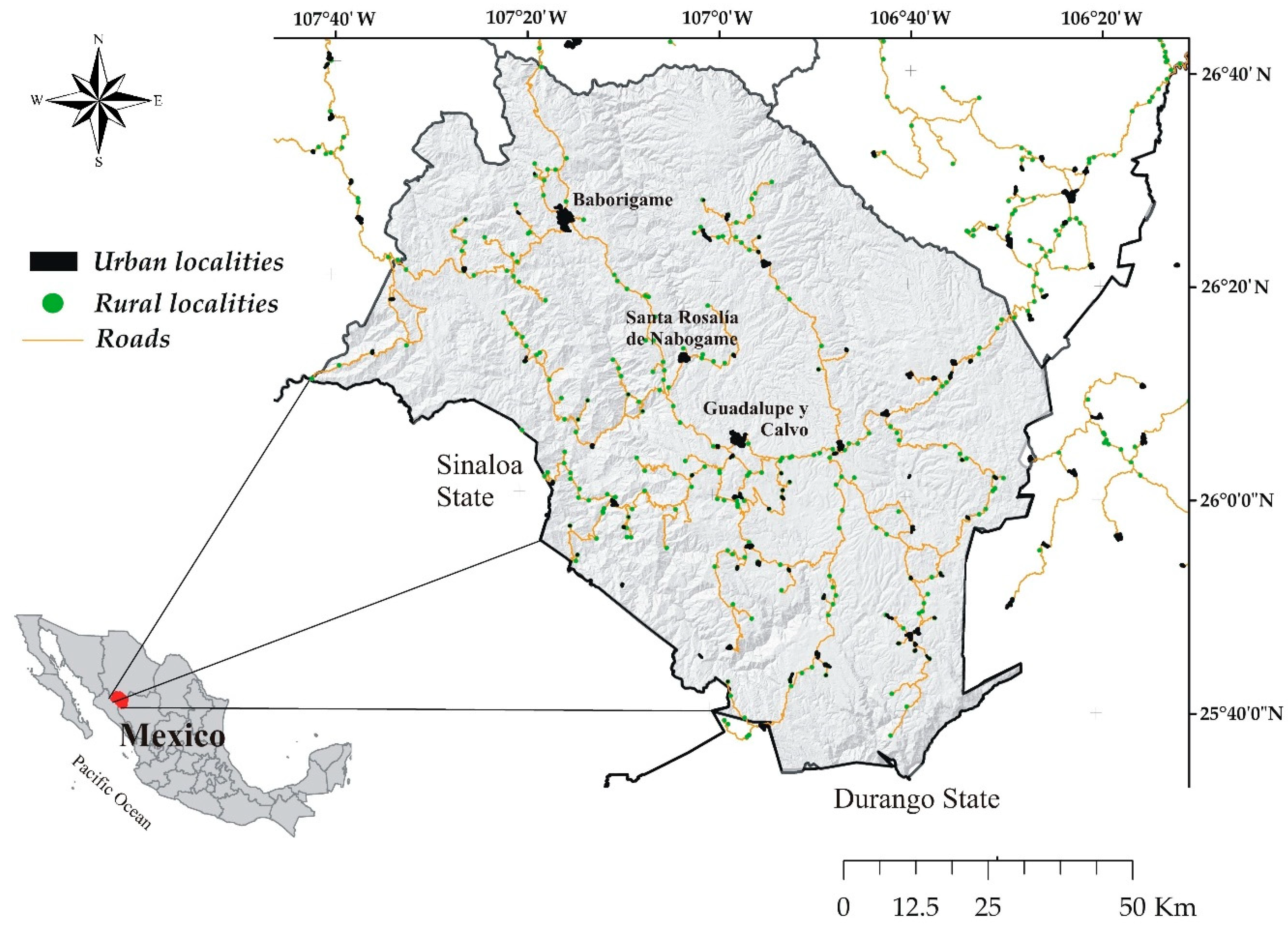
2.1. Study Area
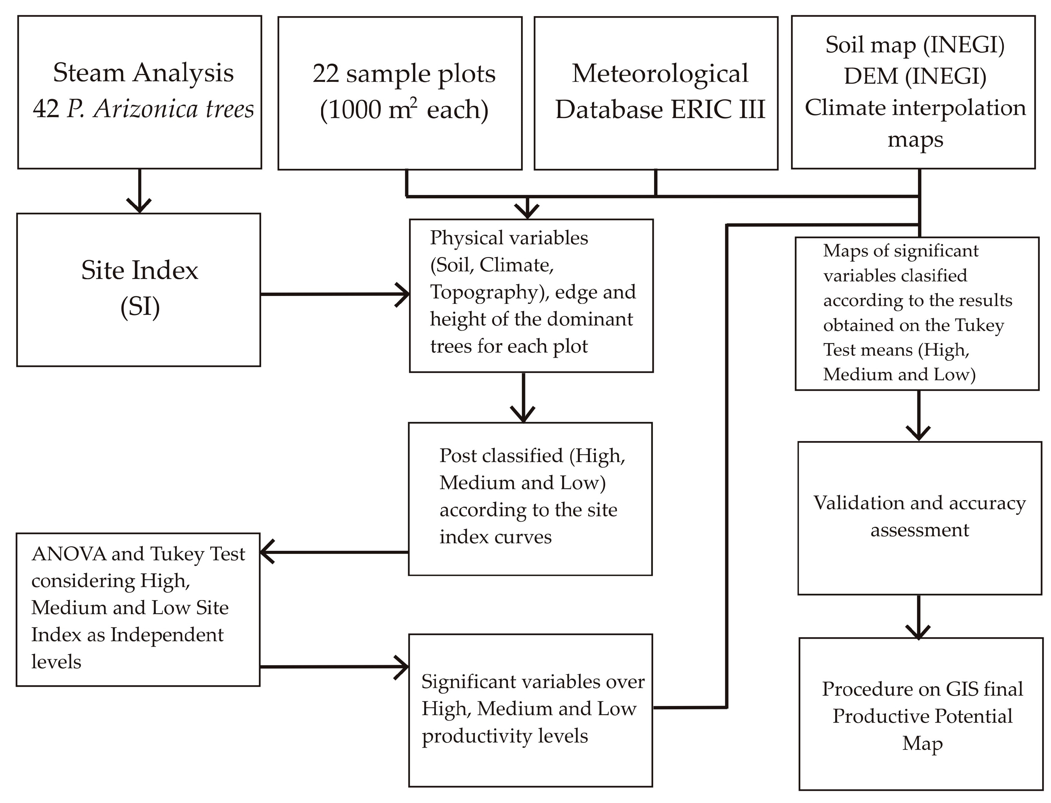
2.2. Methodological Outline and Data
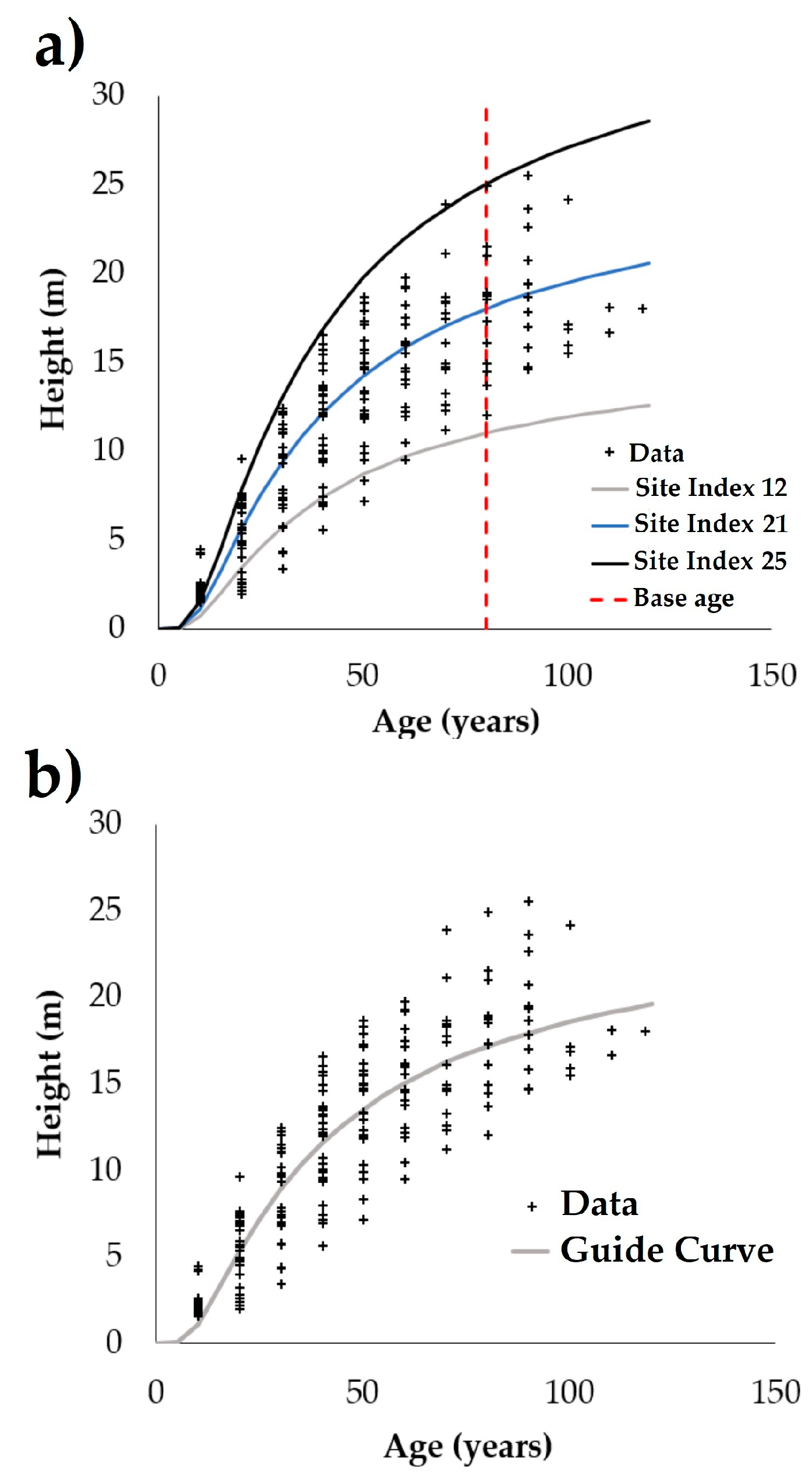
2.3. Site Index Model
2.4. Analysis
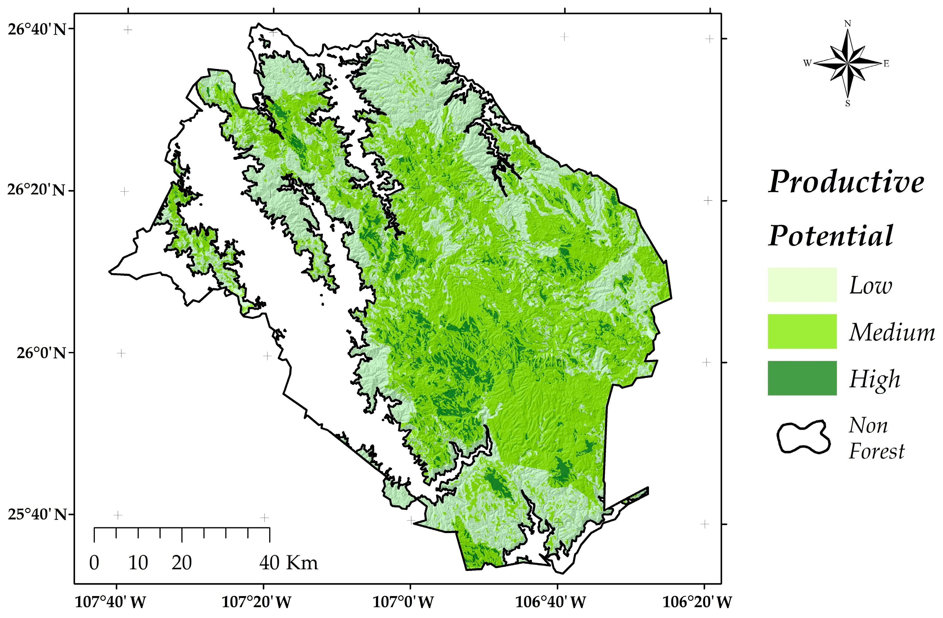
3. Results
4. Discussion
5. Conclusions and Recommendations
Author Contributions
Funding
Conflicts of Interest
References
- Weiskittel, A.R.; Crookston, N.L.; Radtke, P.J. Linking climate, gross primary productivity, and site index across forests of the western United States. Can. J. For. Res. 2011, 41, 1710–1721. [Google Scholar] [CrossRef]
- Babulo, B.; Muys, B.; Nega, F.; Tollens, E.; Nyssen, J.; Deckers, J.; Mathijs, E. The economic contribution of forest resource use to rural livelihoods in Tigray, Northern Ethiopia. For. Policy. Econ. 2009, 11, 109–117. [Google Scholar] [CrossRef]
- Youn, Y.C. Use of forest resources, traditional forest-related knowledge and livelihood of forest dependent communities: Cases in South Korea. For. Ecol. Manag. 2009, 257, 2027–2034. [Google Scholar] [CrossRef]
- Hall, R.J.; Skakun, R.S.; Arsenault, E.J.; Case, B.S. Modeling forest stand structure attributes using Landsat ETM+ data: Application to mapping of aboveground biomass and stand volume. For. Ecol. Manag. 2006, 225, 378–390. [Google Scholar] [CrossRef]
- Mas, J.F.; Velázquez, A.; Díaz-Gallegos, J.R.; Mayorga-Saucedo, R.; Alcántara, C.; Bocco, G.; Castro, R.; Fernandez, T.; Pérez-Vega, A. Assessing land use/cover changes: A nationwide multidate spatial database for Mexico. Int. J. Appl. Earth. Obs. 2004, 5, 249–261. [Google Scholar] [CrossRef]
- Hansen, M.C.; Potapov, P.V.; Moore, R.; Hancher, M.; Turubanova, S.A.A.; Tyukavina, A.; Thau, D.; Stehman, S.V.; Goetz, S.J.; Loveland, T.R.; et al. High-resolution global maps of 21st-century forest cover change. Science 2013, 342, 850–853. [Google Scholar] [CrossRef] [PubMed]
- Lindner, M.; Maroschek, M.; Netherer, S.; Kremer, A.; Barbati, A.; Garcia-Gonzalo, J.; Seidi, R.; Delzon, S.; Corona, P.; Kolström, M.; et al. Climate change impacts, adaptive capacity, and vulnerability of European forest ecosystems. For. Ecol. Manag. 2010, 259, 698–709. [Google Scholar] [CrossRef]
- Taubert, F.; Fischer, R.; Groeneveld, J.; Lehmann, S.; Müller, M.S.; Rödig, E.; Wiegand, T.; Huth, A. Global patterns of tropical forest fragmentation. Nature 2018, 554, 519–522. [Google Scholar] [CrossRef]
- Návar, J. Allometric equations for tree species and carbon stocks for forests of northwestern Mexico. For. Ecol. Manag. 2009, 257, 427–434. [Google Scholar] [CrossRef]
- Altun, L.; Başkent, E.Z.; Bakkaloğlu, M.; Günlü, A.; Kadioğullari, A.İ. Comparing methods for determining forest sites: A case study in Gümüşhane-Karanlıkdere forest. Eur. J. For. Res. 2008, 127, 395. [Google Scholar] [CrossRef]
- Kodani, E.; Tarumi, A.; Awaya, Y. Estimating Forest Productivity of Manmade Coniferous Forest Stands Using Low Density Lidar. Int. Arch. Photogramm. Remote Sens. Spat. Inf. Sci. 2010, 38, 628–630. [Google Scholar]
- Ercanli, I.; Gunlu, A.; Altun, L.; Zeki Baskent, E. Relationship between site index of oriental spruce [Picea orientalis (L.) Link] and ecological variables in Maçka, Turkey. Scand. J. For. Res. 2008, 23, 319–329. [Google Scholar] [CrossRef]
- Mohamed, A.; Reich, R.M.; Khosla, R.; Aguirre-Bravo, C.; Briseño, M.M. Influence of climatic conditions, topography and soil attributes on the spatial distribution of site productivity index of the species rich forests of Jalisco, Mexico. J. For. R. 2014, 25, 87–95. [Google Scholar] [CrossRef]
- Avery, T.E.; Burkhart, H.E. Forest Measurements, 5th ed.; Waveland Press: Long Grove, IL, USA, 2015; pp. 211–229. ISBN 1-4786-2908-8. [Google Scholar]
- Richardson, B.; Skinner, M.F.; West, G. The role of forest productivity in defining the sustainability of plantation forests in New Zealand. For. Ecol. Manag. 1999, 122, 125–137. [Google Scholar] [CrossRef]
- Fox, D.M.; Maselli, F.; Carrega, P. Using SPOT images and field sampling to map burn severity and vegetation factors affecting post forest fire erosion risk. Catena 2008, 75, 326–335. [Google Scholar] [CrossRef]
- Runkle, J.R. Guidelines and Sample Protocol for Sampling Forest Gaps; Department of Agriculture, Forest Service, Pacific Northwest Research Station: Portland, OR, USA, 1992; p. 283. [Google Scholar]
- Vásconez, N.L.; Sevilla, H.C. Uso De Los Sensores Remotos En Mediciones Forestales. Eur. Sci. J. 2018, 14. [Google Scholar] [CrossRef]
- Stearns-Smith, S. Making sense of site index estimates in British Columbia: A quick look at the big picture. J. Ecosyst. Manag. 2001, 1, 1–4. [Google Scholar]
- Skovsgaard, J.P.; Vanclay, J.K. Forest site productivity: A review of the evolution of dendrometric concepts for even-aged stands. Forestry 2008, 81, 13–31. [Google Scholar] [CrossRef]
- Carmean, W.H. Forest site quality evaluation in the United States. Adv. Agron. 1975, 27, 207–269. [Google Scholar] [CrossRef]
- Shen, C.; Lei, X.; Liu, H.; Wang, L.; Liang, W. Potential impacts of regional climate change on site productivity of Larix olgensis plantations in northeast China. iForest 2015, 8, 642. [Google Scholar] [CrossRef]
- Farrelly, N.; Dhubhain, A.N.; Nieuwenhuis, M. Site index of Sitka spruce (Picea sitchensis) in relation to different measures of site quality in Ireland. Can. J. For. Res. 2011, 41, 265–278. [Google Scholar] [CrossRef]
- Bueis, T.; Bravo, F.; Pando, V.; Turrión, M.B. Relationship between environmental parameters and Pinus sylvestris L. site index in forest plantations in northern Spain acidic plateau. iForest 2016, 9, 394. [Google Scholar] [CrossRef]
- Sharma, R.P.; Brunner, A.; Eid, T. Site index prediction from site and climate variables for Norway spruce and Scots pine in Norway. Scand. J. For. Res. 2012, 27, 619–636. [Google Scholar] [CrossRef]
- Socha, J.; Pierzchalski, M.; Balazy, R.; Ciesielski, M. Modelling top height growth and site index using repeated laser scanning data. For. Ecol. Manag. 2017, 406, 307–317. [Google Scholar] [CrossRef]
- Clutter, J.L.; Fortson, J.C.; Peinar, L.V.; Bailey, R.L. Timber Management: A quantitative Approach, 1st ed.; Wiley: New York, NY, USA, 1983; pp. 1–333. ISBN 978-0894647475. [Google Scholar]
- Meyer, H.A. A mathematical expression for height curves. J. For. 1940, 38, 415–420. [Google Scholar]
- Crookston, N.L.; Rehfeldt, G.E.; Dixon, G.E.; Weiskittel, A.R. Addressing climate change in the forest vegetation simulator to assess impacts on landscape forest dynamics. For. Ecol. Manag. 2010, 260, 1198–1211. [Google Scholar] [CrossRef]
- Aertsen, W.; Kint, V.; Van Orshoven, J.; Muys, B. Evaluation of modelling techniques for forest site productivity prediction in contrasting ecoregions using stochastic multicriteria acceptability analysis (SMAA). Ann. For. Sci. 2011, 26, 929–937. [Google Scholar] [CrossRef]
- Brandl, S.; Falk, W.; Klemmt, H.J.; Stricker, G.; Bender, A.; Rötzer, T.; Pretzsch, H. Possibilities and limitations of spatially explicit site index modelling for spruce based on National Forest Inventory data and digital maps of soil and climate in Bavaria (SE Germany). Forests 2014, 5, 2626–2646. [Google Scholar] [CrossRef]
- González, J.G.Á.; González, A.D.R.; Soalleiro, R.R.; Anta, M.B. Ecoregional site index models for Pinus pinaster in Galicia (northwestern Spain). Ann. For. Sci. 2005, 62, 115–127. [Google Scholar] [CrossRef]
- Mestre, S.; Alegria, C.; Albuquerque, M.T.D.; Goovaerts, P. Developing an index for forest productivity mapping-A case study for maritime pine production regulation in Portugal. Rev. Árvore 2017, 41. [Google Scholar] [CrossRef]
- Goodchild, M.; Haining, R.; Wise, S. Integrating GIS and spatial data analysis: Problems and possibilities. Int. J. Geogr. Inf. Syst. 1992, 6, 407–423. [Google Scholar] [CrossRef]
- Pelissari, A.L.; Caldeira, S.F.; Figueiredo Filho, A.; Amaral, M.S. Propostas de mapeamentos da capacidade produtiva de sítios florestais por meio de análises geoestatísticas. Sci. For. 2015, 43, 601–608. [Google Scholar]
- Ollinger, S.V.; Aber, J.D.; Federer, A. Estimating regional forest productivity and walter yield using an ecosystem model linked to a GIS. Landsc. Ecol. 1998, 13, 323–334. [Google Scholar] [CrossRef]
- Payn, T.W.; Hill, R.B.; HÖck, BK.; Skinner, M.F.; Thorn, A.J.; Rijkse, W.C. Potential for the use of GIS and spatial analysis techniques as tools for monitoring changes in forest productivity and nutrition, a New Zealand example. For. Ecol. Manag. 1999, 122, 187–196. [Google Scholar] [CrossRef]
- Korkalainen, T.; Laurén, A. Using phytogeomorphology, cartography and GIS to explain forest site productivity expressed as tree height in southern and central Finland. Geomorphology 2006, 74, 271–284. [Google Scholar] [CrossRef]
- Minowa, Y.; Suzuki, N.; Tanaka, K. Estimation of site indices with an artificial neural network (in Japanese with English abstract). Jpn. J. For. Plan. 2005, 39, 23–38. [Google Scholar]
- Waring, R.H.; Coops, N.C.; Mathys, A.; Hilker, T.; Latta, G. Process-based modeling to assess the effects of recent climatic variation on site productivity and forest function across Western North America. Forests 2014, 5, 518–534. [Google Scholar] [CrossRef]
- Tang, D.; Bian, F. Forest Site Evaluation Based on GIS and Kriging. In Proceedings of the First International Conference on Information Science and Engineering, Nanjing, Jiangsu, China, 26–28 December 2009. [Google Scholar]
- Wulder, M.; White, J.; Fournier, R.; Luther, J.; Magnussen, S. Spatially explicit large area biomass estimation: Three approaches using forest inventory and remotely sensed imagery in a GIS. Sensors 2008, 8, 529–560. [Google Scholar] [CrossRef]
- Corral-Rivas, J.J.; Alvarez-Gonzalez, J.G.; Ruız-Gonzalez, A.D.; Von-Gadow, K. Compatible height and site index models for five pine species in El Salto, Durango (Mexico). For. Ecol. Manag. 2004, 201, 145–160. [Google Scholar] [CrossRef]
- Alanis Morales, H.; Navar, J.; Dominguez, P.A. The effect of prescribed burning on surface runoff in a pine forest stand of Chihuahua, Mexico. For. Ecol. Manag. 2000, 137, 199–207. [Google Scholar] [CrossRef]
- Tarango, J.A.; Valdez, R.; Zwank, P.J.; Cardenas, M. Mexican spotted owl characteristics in Southwestern Chihuahua, Mexico. Southwest. Nat. 1997, 42, 132–136. [Google Scholar]
- Crecente-Campo, F.; Corral-Rivas, J.J.; Vargas-Larreta, B.; Wehenkel, C. Can random components explain differences in the height–diameter relationship in mixed uneven-aged stands? Ann. For. Sci. 2014, 71, 51–70. [Google Scholar] [CrossRef]
- Chávez Rodriguez, N. Estudio Regional Forestal. Asociación Regional de Silvicultores De Guadalupe y Calvo, A.C. Unidad De Manejo Forestal No. 0808 Guadalupe Y Calvo, Chihuahua. Available online: http://www.conafor.gob.mx:8080/documentos/docs/9/1147ERF_UMAFOR0808.pdf (accessed on 20 December 2016).
- British Columbia Forest Productivity Council (BCFPC). Minimum Standards and Stem Analysis Procedures for Site Index Research. Forest Productivity Council; BCFPC: Victoria, BC, Canada, 1998; pp. 1–13. [Google Scholar]
- Instituto Mexicano de Tecnología del Agua (IMTA). Banco de datos histórico nacional del Servicio Meteorológico Nacional. Base de datos digital; Instituto Mexicano de Tecnología del Agua: Mexico City, Mexico, 2006. [Google Scholar]
- Palahí, M.; Tome, M.; Pukkala, T.; Trasobares, A.; Montero, G. Site index model for Pinus sylvestris in northeast Spain. For. Ecol. Manag. 2004, 187, 35–47. [Google Scholar] [CrossRef]
- SAS Institute Help and Documentation, version 9.1.3; SAS Institute Inc.: Cary, NC, USA, 2006.
- Onyekwelu, J.C. Site index curves for site quality assessment of nauclea diderrichii monoculture plantations in Omo Forest Reserve, Nigeria. J. Trop. For. Sci. 2005, 17, 532–542. [Google Scholar]
- ArcGIS Desktop: 10.2. Environmental Systems Research Institute (ESRI) Home Page. Available online: www.esri.com (accessed on 26 September 2017).
- Instituto Nacional de Estadística, Geografía e Informática (INEGI). Continúo de elevaciones mexicano 3.0. Available online: http://www.inegi.org.mx/geo/contenidos/datosrelieve/continental/Descarga.aspx (accessed on 8 December 2016).
- Burrough, P.A.; McDonnell, R. Principles of Geographical Information Systems, 2nd ed.; Oxford University Press: Oxford, UK, 1998; pp. 1–356. ISBN 9780198233664. [Google Scholar]
- Congalton, R.G. A review of assessing the accuracy of classifications of remotely sensed data. Remote Sens. Environ. 1991, 37, 35–46. [Google Scholar] [CrossRef]
- Monserud, R.A.; Leemans, R. Comparing global vegetation maps with the Kappa statistic. Ecol. Model. 1992, 62, 275–293. [Google Scholar] [CrossRef]
- Zimmerman, D.L.; Nunez-Anton, V. Parametric modelling of growth curve data: An overview. Test 2001, 10, 1–73. [Google Scholar] [CrossRef]
- Seynave, I.; Gégout, J.C.; Hervé, J.C.; Dhôte, J.F.; Drapier, J.; Bruno, É.; Dumé, G. Picea abies site index prediction by environmental factors and understorey vegetation: A two-scale approach based on survey databases. Can. J. For. Res. 2005, 35, 1669–1678. [Google Scholar] [CrossRef]
- Bolte, A.; Ammer, C.; Löf, M.; Madsen, P.; Nabuurs, G.J.; Schall, P.; Spathelf, P.; Rock, J. Adaptive forest management in central Europe: Climate change impacts, strategies and integrative concept. Scand. J. For. Res. 2009, 24, 473–482. [Google Scholar] [CrossRef]
- Curt, T.; Bouchaud, M.; Agrech, G. Predicting site index of Douglas-fir plantations from ecological variables in the Massif Central area of France. For. Ecol. Manag. 2001, 149, 61–74. [Google Scholar] [CrossRef]
- Solberg, S.; Dobbertin, M.; Reinds, G.J.; Lange, H.; Andreassen, K.; Fernandez, P.G.; Hildingsson, A.; de Vries, W. Analyses of the impact of changes in atmospheric deposition and climate on forest growth in European monitoring plots: A stand growth approach. For. Ecol. Manag. 2009, 258, 1735–1750. [Google Scholar] [CrossRef]
- Johansson, T. Site index curves for young hybrid larch growing on former farmland in Sweden. Forests 2012, 3, 723–735. [Google Scholar] [CrossRef]
- Günlü, A.; Baskent, E.Z.; Kadiogullari, A.İ.; Ercanli, İ. Classifying oriental beech (Fagus orientalis Lipsky.) forest sites using direct, indirect and remote sensing methods: A case study from Turkey. Sensors 2008, 8, 2526–2540. [Google Scholar] [CrossRef] [PubMed]
- Adams, J.P.; Matney, T.G.; Land, S.B., Jr.; Belli, K.L.; Duzan, H.W., Jr. Incorporating genetic parameters into a loblolly pine growth-and-yield model. Can. J. For. Res. 2006, 36, 1959–1967. [Google Scholar] [CrossRef]
- Vicca, S.; Luyssaert, S.; Penuelas, J.; Campioli, M.; Chapin, F.S., III; Ciais, P.; Heinemeyer, A.; Högberg, P.; Kutsch, W.L.; Law, B.E.; et al. Fertile forests produce biomass more efficiently. Ecol. Lett. 2012, 15, 520–526. [Google Scholar] [CrossRef] [PubMed]
- Reich, R.M.; Bonham, C.D.; Aguirre-Bravo, C.; Chazaro-Basañeza, M. Patterns of tree species richness in Jalisco, Mexico: Relation to topography, climate and forest structure. Plant Ecol. 2010, 210, 67–84. [Google Scholar] [CrossRef]
- Peters, E.B.; Wythers, K.R.; Bradford, J.B.; Reich, P.B. Influence of disturbance on temperate forest productivity. Ecosystems 2013, 16, 95–110. [Google Scholar] [CrossRef]
- Coops, N.C.; Waring, R.H.; Hilker, T. Prediction of soil properties using a process-based forest growth model to match satellite-derived estimates of leaf area index. Remote Sens. Environ. 2012, 126, 160–173. [Google Scholar] [CrossRef]
- Véga, C.; St-Onge, B. Mapping site index and age by linking a time series of canopy height models with growth curves. For. Ecol. Manag. 2009, 257, 951–959. [Google Scholar] [CrossRef]
- Gómez-Tagle, R.A. Levantamiento de suelos del Campo Experimental Forestal Barranca de Cupatitzio y sus relaciones con la vegetación de confieras. Master’s Thesis, Universidad Nacional Autonoma de Mexico, México City, Mexico, 1985. [Google Scholar]
- Fontes, L.; Tomé, M.; Thompson, F.; Yeomansi, A.; Sales, L.J.; Savilli, P. Modelling the Douglas-fir (Pseudotsuga menziesii (Mirb.) Franco) site index from site factors in Portugal. Forestry 2003, 76, 491–507. [Google Scholar] [CrossRef]
- Aertsen, W.; Kint, V.; Muys, B.; Van Orshoven, J. Effects of scale and scaling in predictive modelling of forest site productivity. Environ. Modell. Softw. 2012, 31, 19–27. [Google Scholar] [CrossRef]
- Mitsuda, Y.; Ito, S.; Sakamoto, S. Predicting the site index of sugi plantations from GIS-derived environmental factors in Miyazaki Prefecture. J. For. R. 2007, 12, 177–186. [Google Scholar] [CrossRef]
- Johnsen, K.; Samuelson, L.; Teskey, R.; McNulty, S.; Fox, T. Process models as tools in forestry research and management. For. Sci. 2001, 47, 2–8. [Google Scholar]
- Rodhouse, T.J.; Irvine, K.M.; Sheley, R.L.; Smith, B.S.; Hoh, S.; Esposito, D.M.; Mata-Gonzalez, R. Predicting foundation bunchgrass species abundances: Model-assisted decision-making in protected-area sagebrush steppe. Ecosphere 2014, 5, 1–16. [Google Scholar] [CrossRef]


| Variable | Average | Max Value | Min Value |
|---|---|---|---|
| Above sea level altitude (m) | 2314 | 3020 | 1690 |
| Slope (%) | 31 | 85 | 5 |
| A-Horizon (cm) | 33 | 97 | 3 |
| Rockiness (% Cover) | 23 | 78 | 0 |
| Bare soil (% Cover) | 13 | 85 | 0 |
| Litter depth (cm) | 2 | 9.5 | 0.3 |
| Min temperature °C | 5 | 13 | 1 |
| Max temperature °C | 23 | 32 | 17 |
| Precipitation (mm) | 898 | 1248 | 576 |
| DBH (cm) | Height (m) | |||||||
|---|---|---|---|---|---|---|---|---|
| Age | Mean | St. Dev. | Min | Max | Mean | St. Dev. | Min | Max |
| 10 | 4.3 | 2.5 | 3.1 | 10.6 | 2.5 | 0.9 | 1.6 | 4.6 |
| 20 | 8.9 | 4.2 | 5.5 | 16.6 | 5.5 | 1.9 | 2.1 | 9.7 |
| 30 | 13.8 | 5.1 | 4.3 | 21.6 | 8.8 | 2.8 | 3.5 | 12.5 |
| 40 | 18.7 | 5.3 | 9.3 | 26.7 | 11.7 | 3.0 | 5.7 | 16.6 |
| 50 | 22.6 | 5.4 | 12.6 | 32.2 | 13.6 | 2.9 | 7.2 | 18.7 |
| 60 | 26.3 | 5.1 | 16.0 | 34.4 | 15.5 | 3.0 | 9.6 | 19.8 |
| 70 | 28.1 | 5.3 | 20.1 | 35.0 | 16.4 | 3.5 | 11.3 | 23.9 |
| 80 | 31.4 | 6.4 | 23.9 | 40.9 | 17.8 | 3.4 | 12.1 | 25.0 |
| 90 | 33.1 | 6.1 | 26.2 | 43.7 | 19.6 | 3.5 | 14.7 | 25.6 |
| Schumacher | SSE | MSE | RMSE | R2 | R2ajus | DW | Parameter | Estimate | Approx Std Err | t Value | Approx Pr > |t| |
|---|---|---|---|---|---|---|---|---|---|---|---|
| 554.6 | 2.6287 | 1.6213 | 0.9258 | 0.9247 | 1.3877 | β0 | 25.5103 | 1.0893 | 23.42 | <0.0001 | |
| β1 | 31.7767 | 1.8258 | 17.40 | <0.0001 | |||||||
| p1d | 0.9656 | 0.0208 | 46.39 | <0.0001 | |||||||
| p2d | 0.8785 | 0.0251 | 34.95 | <0.0001 |
| Variable | Statistics | Productivity Level | ||||||||
|---|---|---|---|---|---|---|---|---|---|---|
| Low | Medium | High | ||||||||
| SS | MSE | Fc | Pr > F | Mean | Stdv | Mean | Stdv | Mean | Stdv | |
| Slope (degree) ** | 0.215 | 0.107 | 3.999 | 0.020 | 37A | 15 | 30A | 15 | 12B | 8 |
| Soil depth (cm) ** | 527.354 | 263.677 | 0.698 | 0.012 | 26A | 18 | 36B | 19 | 44B | 11 |
| Rockiness (%) | 0.154 | 0.077 | 2.332 | 0.100 | 29 | 2 | 22 | 17 | 21 | 18 |
| Bare soil (%) | 0.002 | 0.001 | 0.056 | 0.945 | 12 | 1 | 13 | 14 | 13 | 17 |
| A-Horizon (cm) | 4.311 | 2.156 | 2.039 | 0.133 | 1.5 | 0.8 | 1.6 | 0.8 | 1.9 | 1.3 |
| Litter depth (cm) | 0.071 | 0.035 | 0.644 | 0.527 | 0.6 | 0.2 | 0.6 | 0.2 | 0.6 | 0.3 |
| Minimum temperature (°C) ** | 37.378 | 18.689 | 3.261 | 0.041 | 5A | 2 | 4A | 1 | 8B | 3 |
| Maximum temperature (°C) ** | 86.152 | 43.076 | 5.208 | 0.006 | 23A | 3 | 23A | 2 | 18B | 3 |
| Precipitation (mm) * | 1219.023 | 609.511 | 0.043 | 0.096 | 794A | 43 | 897B | 92 | 901B | 116 |
© 2019 by the authors. Licensee MDPI, Basel, Switzerland. This article is an open access article distributed under the terms and conditions of the Creative Commons Attribution (CC BY) license (http://creativecommons.org/licenses/by/4.0/).
Share and Cite
Martínez-Salvador, M.; Mata-Gonzalez, R.; Pinedo-Alvarez, A.; Morales-Nieto, C.R.; Prieto-Amparán, J.A.; Vázquez-Quintero, G.; Villarreal-Guerrero, F. A Spatial Forestry Productivity Potential Model for Pinus arizonica Engelm, a Key Timber Species from Northwest Mexico. Sustainability 2019, 11, 829. https://doi.org/10.3390/su11030829
Martínez-Salvador M, Mata-Gonzalez R, Pinedo-Alvarez A, Morales-Nieto CR, Prieto-Amparán JA, Vázquez-Quintero G, Villarreal-Guerrero F. A Spatial Forestry Productivity Potential Model for Pinus arizonica Engelm, a Key Timber Species from Northwest Mexico. Sustainability. 2019; 11(3):829. https://doi.org/10.3390/su11030829
Chicago/Turabian StyleMartínez-Salvador, Martin, Ricardo Mata-Gonzalez, Alfredo Pinedo-Alvarez, Carlos R. Morales-Nieto, Jesús A. Prieto-Amparán, Griselda Vázquez-Quintero, and Federico Villarreal-Guerrero. 2019. "A Spatial Forestry Productivity Potential Model for Pinus arizonica Engelm, a Key Timber Species from Northwest Mexico" Sustainability 11, no. 3: 829. https://doi.org/10.3390/su11030829
APA StyleMartínez-Salvador, M., Mata-Gonzalez, R., Pinedo-Alvarez, A., Morales-Nieto, C. R., Prieto-Amparán, J. A., Vázquez-Quintero, G., & Villarreal-Guerrero, F. (2019). A Spatial Forestry Productivity Potential Model for Pinus arizonica Engelm, a Key Timber Species from Northwest Mexico. Sustainability, 11(3), 829. https://doi.org/10.3390/su11030829