Effects of Kyoto Protocol on CO₂ Emissions: A Five-Country Rolling Regression Analysis

Abstract

The current study illustrated the time variance of turning points in the relationship between carbon emissions and income to resolve heated debate on the different responsibility to climate change with 1950–2010 data of five development diversity countries—three developed countries (Germany, Italy, and Japan) and one developing country (India) and one newly industrialized economy (Taiwan). The article also examines the impact of the crisis on emission. The time-varying patterns in the turning points on environmental Kuznets curves (EKCs) were observed by a rolling regression technique with 1950–2010 data regarding the per capita CO₂ emissions caused by fossil fuel combustion and the incomes of the countries. Several empirical findings were revealed from this analysis. Per capita CO₂ emissions commonly decreased with varying magnitudes in the five countries over time. The EKC hypothesis regarding the CO₂ emissions is affirmed again in this study. The announcement effects associated with the Kyoto Protocol was evidenced. As indicated by the occurring GDP of the turning point, there is a strong reduction trend in the income level of the turning points right before the years of Kyoto Protocol; and this decreasing trend nearly ended as the Kyoto protocol approached its end, except in Germany, where the occurring income of the turning points continued to have a decreasing trend. Although the global financial crisis had its effects in the world, the impacts on carbon dioxide emissions vary across countries.

1. Introduction

The increase in the number of disasters caused by global warming prompted the United Nations Framework Convention on Climate Change (UNFCCC) to establish the Kyoto Protocol, the first international treaty for reducing excessive greenhouse gas emissions [1,2,3], to mitigate global warming. To prevent harmful changes from global warming catalyzed by human activity, the Kyoto Protocol was signed in 1997 and enacted in 2005. The Kyoto Protocol is supported by most countries, many of which have striven to amend and update their domestic policies in response to global concerns and have passed voluntary legislation or ratifications based on domestic public opinion. Many countries have integrated various regional and domestic policies enacted before and after introduction of the Kyoto Protocol.

Increases of the economic activities in history are regarded as the culprit for observed global warming [4]. The developed countries in Annex I in the Kyoto Protocol were obligated to reduce CO₂ emissions in its first commitment period, 2008–2012, whereas Non-Annex I developing countries with low or mid-level average incomes had no such binding emission target.

The first commitment period, 2008–2012, has passed after the 2012 Doha Amendment [5]. While negotiating potential amendments to the Kyoto Protocol, countries have disputed how to maintain a low atmospheric CO₂ concentration. Under the Kyoto Protocol, developed countries must determine how to reduce disparity between their binding targets and actual reductions, whereas developing countries have no such direct binding targets. Huang et al. [6] argued that because of their rapidly developing economies, some developing countries may emit large concentrations of CO₂ unless relevant voluntary initiatives are employed. From this perspective, amendments to the Kyoto Protocol require both developed and developing countries to voluntarily reduce their CO₂ emissions. At the 21st conference of parties (COP 21) in Paris, parties to the UNFCCC reached a landmark agreement, the so-called “Paris Agreement”, to accelerate and intensify the actions and investments for a sustainable low carbon future; and the rules for the Paris Agreement were elaborated at the COP 24 to the UNFCCC held in 2018 [7,8]. To reveal the actual effects generated from the first commitment period of Kyoto Protocol is especially important as there are heated debates on the responsibility taken by the countries with income and development diversity, since countries in different income levels might have divergent emission potentiality and mitigation capability. It is worthwhile to develop the practice and research on income development among countries and make policy implications.

To understand how to address the aforementioned controversy and divergent views regarding roles and responsibilities undertaken to reduce CO₂ emissions, this study selected five countries to investigate the effects of the Kyoto Protocol on CO₂ emissions. With different economic structures at various stages of economic development, here valuable climate policy implications are drawn from the empirical evidences with respect to the country’s emission potentiality and their mitigation capability with their divergence in income level and their economic development. The five countries in the present study are Germany, Italy, Japan, India, and Taiwan, all of which have differential responsibilities in reducing CO₂ emissions in the first commitment period of the Kyoto Protocol. Germany, Italy, and Japan belong to Annex I of the treaty, and thus have emission targets, whereas India is a developing country without a binding target. On the contrary, the newly developed economy, Taiwan, is a party undefined in the protocol.

How Japan, Germany, and Italy’s response in their trends to carbon emissions are of interest. Since EU countries have model initiatives to the mitigation of global warming and the European Union is one of the most actively involved parties in CO₂ emission reduction under the Kyoto Protocol [9], it is interesting to pick the top two in the manufacturing scale [10] among its member states, Germany and Italy, in this investigation. Germany has the largest national economy in Europe. Its industry sector contributes around 30% of the national outputs. Italy is also a large manufacturer and overall the second in EU behind Germany (Eurostat, 2019). Moreover, Japan is the largest developed economy in Asia, and the Kyoto Protocol was adopted in Kyoto, Japan, on 11 December 1997. Therefore, this study picked three single countries among them on the purpose to (1) show countries of high fossil-fuel reliance reduce the global risk of catastrophic climate change, to (2) demonstrate the decarbonization trends of the potential devoted model countries (two EU countries and Japan).

Income is typically among the most critical factors affecting policymaking in a country and is the most commonly-used determinant of human-induced CO₂ emissions. The persistent importance of the income variables in an environmental Kuznets curves (EKC) study was proposed by econometrists, Müller-Fürstenberger and Wagner [11,12]; and a reduced form EKC model was suggested by Vollebergh et al. [13]. A reduced form of EKC model specification was adopted in this study. Some other recommended literature [14,15,16] include more relevant variables in EKC study and make respective conclusions on the significances of these variables. For these perspectives, after thoroughly reviewing and discussing these literature (in the latter sections), the practice of this study was to takes into account the development diversity of the countries surveyed.

In addition to examining the links between carbon emissions and income, the present study also examined the impacts of the financial crisis on the emissions trend during the first commitment of Kyoto Protocol. There are contradictory ideas on the emission response to the economic recessions. On the purpose to combat global warming, the CO₂ emissions mitigate with declined economic production. On the contrary, countries might increase their energy use, and therefore their carbon emissions, to survive in the crisis, to recover from recession, and/or to support their future economic growth. From these perspectives, the present study demonstrated how the trajectory of CO₂ emission trends changes during the period of global financial crisis. It is interesting to probe the emission behavior of the countries to justify whether there is downturn (or upturn) trends to the volume of carbon emissions.

The time transition of turning points on inverted U-shaped EKCs can serve as an indicator of trends of CO₂-emission pattern. The EKC turning points are a viable indicator of policy effects on the study on a panel of homogeneity countries in their income, energy, and policy, and therefore also to individual countries with persistent economic structure. The individual country investigation in the present study is far away from the case of Richmond and Kaufmann [14,15]. Their arguments regarding the weak statistical significance are, in fact, valid merely in the case adopting cross-country panel data of economic heterogeneity like their research.

The CO₂ reduction effects of the chosen five countries are compared in this study by using the technique of rolling regression to compute parameters and assess the time trends of consistency of economic patterns—changes in the turning points of an EKC by rolling the subsamples [17,18,19]. Because the economies and population sizes of these five countries vary substantially, CO₂ emission levels and income variables were measured in per capita units to facilitate convenient comparison with data retrieved from reliable sources.

The estimated shapes of EKCs and the evaluated turning points in the relationship between per capita CO₂ emissions and per capita income levels were used to demonstrate the equilibrium path of income and emissions in order to illustrate changes caused by each individual country’s public preference, technology, and governmental policies and legislation. In addition, the effects of economic features such as structures and developmental stages belonging to the five countries were addressed.

The remainder of this paper is structured as follows. Section 2 reviews the related literature and Section 3 empirically analyses the rolling regression for the transition of the EKC turning points under first commitment of Kyoto Protocol. Section 4 presents the econometric analysis outcomes. Section 5 discusses the empirical results. Section 6 provides a conclusion.

2. Literature Review

2.1. EKC Model

A huge volume of literature are on the study concerning the EKC issues. Some key literature, but not all, are reviewed and compared in this paper where appropriate. Since the EKCs were first proposed by Grossman and Krueger [20,21], a large number of pollutants and environmental degradation indicators, including CO₂ emissions, had been examined its EKC relationship with income. However, regarding a wide variety of divergent environmental degradations indicators, there is no persistent consensus on the EKC relationship and studies have debated the existence of the inverted U-shaped EKC model. Shafik [22] illustrated a monotonically increasing relationship, as observed during the uphill period of an EKC curve; moreover, de Bruyn et al. [23] and Friedl and Getzner [24] have observed N-shaped curves due to historical events.

However, many researchers have concluded that per capita CO₂ emissions—an indicator of a degrading environment—demonstrate an inverted U-shaped EKC as income increases. Stefanski [25] and Chen [26] have affirmed inverted U-shaped EKCs in the relationship between per capita CO₂ emissions and per capita income.

Chen [26] argued that the effects of the embedded energy cost in an economy have driven the decreasing in the slopes of the EKC of per capita CO₂ emissions, automatically by the market mechanism. The cost of fossil energy is an indirect cost of CO₂ emissions from fossil fuel combustion along the growth trajectory of income increase.

Shafik and Bandopadhyay [27] demonstrated the externality of climate change had induced from accumulated atmospheric concentrations of CO₂ emitted from human activity. This is a classic free rider problem related to CO₂ emissions; no major local costs are associated with the externality of carbon emissions, and all costs in terms of climate change are borne by the rest of the world. They had expressed their concerns regarding the absence of an automatic decrease in incentives embedded in the economy. However, energy costs are the indirect costs of carbon dioxide emissions and valid mitigating incentives of subsequent global warming. Valuable important policy implications would be made after the inverted U-shaped EKC patterns are affirmed again by the present study.

Therefore, EKC quadratic relationship between CO₂ emissions per capita and GDP per capita suggested by Chen [26] and Stefanski [25] are hypothetically tested in the present study. Based on the results of Shafik [22], Cole [28], Park and Lee [29], and Esteve and Tamarit [30], empirical specifications for the relationship between CO₂ emissions and income in the present study are set as linear, quadratic, cubic, or other nonlinear functional forms by extrapolating and interpolating estimated functional specifications for (1) linear relationships, (2) quadratic relationships (EKCs), (3) cubic relationships, and (4) none of the aforementioned relationships.

2.2. The Turning Points

An inverted U-shaped EKC illustrates that after a specific threshold (a turning point) has been exceeded, CO₂ emissions begin to decrease with a steady increase in income [31,32,33,34]. Changes in turning points can indicate changes in trends in EKC quadratic relationships [11,33,35]. Therefore, changes in EKC turning points can reveal trends in the CO₂ emissions of countries of varying status in 1950–2010 under the Kyoto Protocol.

2.3. Reduced-Form EKC Model

Income is typically among the most critical factors affecting policymaking in a country’s climate policy and is the most commonly used determinant of human-induced CO₂ emissions in the EKC studies. Since income has played the most important role in the EKC studies, and persistent importance of the income variables is proposed by Müller-Fürstenberger and Wagner [12], a reduced-form EKC model with income determinants are relevant and often used [13].

2.4. Cross-Country Study on Income Inequity and Other Variables

Some papers have studied the effects of other variables on the CO₂ emissions as adopting EKC models. Coondoo and Dinda [16], Grunewald et al. [4] included cross-country income inequity and make recommendations for the international climate policy. Richmond and Kaufmann [14,15] included energy mix, energy prices among countries for cross-country analysis and make suggestions for the use a EKC turning point to make statistical inference.

2.5. The Statistical Supports on the Turning Points

Richmond and Kaufmann [14,15] found that statistical support for a EKC turning point would be eliminated due to the strong effects from other variables such as energy prices, energy share, model specifications, and levels of economic development as Richmond and Kaufmann [14,15] adopted panel data of the country groups of OECD and non-OECD, respectively. They found weak statistical supports on the turning point for the countries with high income (OECD countries in their study) and no turning point for countries with low income (non-OECD in that study). They had made very strong suggestions to forecasters and policy makers that they should not depend on a turning point in the relationship between income and energy use or carbon emissions.

However, the investigation of Richmond and Kaufmann [14,15] estimated common turning points for the group of income, energy, and policy heterogeneity countries. Their estimations were based on a very strong assumption to deem the heterogeneity countries in the estimated group as a whole with homogeneity properties in relevant domestic policy, energy structure, and economic structure. Their research and the design was rigorous, however, the suggestions are only valid under the specific circumstance of their study.

On the contrary, the EKC turning points were justified as a good indicator for the effects of climate policy in the present study. In my opinion, if the EKC turning point is sensitive to the changes in the data in an empirical study, it would serve as a good policy indicator. This is because where the EKC relationships were consistent, the turning point estimates were stable and did not vary. The estimated turning points are feasible policy indicators by a study on a panel of countries of homogeneity in their income, energy, and policy, so as to individual countries with persistent economic structure; while its statistical significance will be weakened as adopting cross-country panel data of economic heterogeneity like the research of Richmond and Kaufmann [14,15].

Rather than adopting a panel of cross-country analysis, the patterns for CO₂ emissions are investigated in the present study with a focus on the impact of structural productive conditions of individual countries with reference to the relationship between per capita income and harmful emissions. Cross-country comparison is made by comparing the levels and the transitions of occurring income of the EKC turning points of the selected five countries with different responsibility in the first commitment period of Kyoto Protocol, to partially underline the income inequalities among countries. Policy recommendations at global level is made based on the research evidences of estimated turning points and divergence of the economy and the unbalanced international specialization of economic activities.

In fact, the analysis conducted on individual countries in the present research cannot fully consider the interaction and interdependence between countries. Due to the limitations from the research design and length of this present study, this content is reserved for future research.

2.6. Effects from Kyoto Protocol

Many researches are on the effects from Kyoto Protocol. Recent studies had noted that the ratification of the Kyoto Protocol had reduced CO₂ emissions; but Kyoto commitment had reduced the competitiveness of many Kyoto countries and their exports. and most committed parties were far from achieving their binding ceiling targets. Kyoto reduced domestic emissions in committed countries, has not lowered domestic footprints, but increased the share of imported over domestic emissions with a carbon leakage [36,37,38,39,40].

2.7. The Importance of Time Variation and Rolling for a EKC Relationship

The importance of time variation are suggested by Ajmi et al. [41]. They found that there is significant time-varying nexus among the variables under consideration in their study on the relationships between energy consumption, carbon dioxide emissions and gross domestic product in the G7 countries. This study supports the needs of rolling with a time window in this study as we investigated the time trajectory of the turning points.

2.8. Announcement Effects and Anticipated Effects

The announcement effect refers to the fact that the economic behavior changes with the announcement of a future policy. A policy was announced and anticipated, it took effect, and the anticipated international policies of the Kyoto Protocol exerted their influence [42]. An economy starts to respond to a new future policy and changes its behavior before the practical introduction of the policy [43,44]. Accordingly, the effects of a climate policy may occur both before and after its implementation. Since the purpose of this study is aimed to demonstrate the impacts of Kyoto Protocol, it seems appropriate to backwardly extend the study time period to 1950 and allow the current study to demonstrate the announcement effects, as the Kyoto Protocol was adopted on 11 December 1997 and entered into force on 16 February 2005.

3. Empirical Analysis

3.1. Model Specifications

Studies have debated the existence of the inverted U-shaped EKC model; thus, the present empirical study considered linear and cubic functional specifications between per capita CO₂ emissions and per capita income, in addition to a quadratic EKC relationship. With the significance of quadratic functional forms of EKCs, this empirical study applied EKC quadratic functional forms to investigate emission trends in the relationship between per capita CO₂ emissions and per capita income. The cubic and linear specifications were applied when the quadratic terms were nonsignificant.

$$\mathrm{Linear}\mathrm{functions}:lnC{O}_{2t}=\alpha +{\beta }_{1}ln{Y}_t+u_t$$

(1)

$$\mathrm{Quadratic}\mathrm{EKC}\mathrm{functions}:lnC{O}_{2t}=\alpha +{\beta }_{1}ln{Y}_t+{\beta }_2{(ln{Y}_t)}^2+u_t,$$

(2)

$$\mathrm{Cubic}\mathrm{functions}:lnC{O}_{2t}=\alpha +{\beta }_{1}ln{Y}_t+{\beta }_2{(ln{Y}_t)}^2+{\beta }_3{(ln{Y}_t)}^3+u_t,$$

(3)

where lnCO₂ represents per capita CO₂ emissions expressed as a logarithmic value, lnY represents per capita income expressed as a logarithmic value, and $u_t$ is the error term.

This is consistent with the findings suggested by Chen [26] and Stefanski [25] which had suggested a quadratic relationship between CO₂ emissions per capita and GDP per capita. We focused only on the quadratic relationship, and the relationships can be inferred using the signs of coefficients specified in the quadratic specification Equation (2).

(1) ${\beta }_1$ > 0 and ${\beta }_2=0$ indicates a monotonically increasing linear relationship.

(2) ${\beta }_1$ < 0 and ${\beta }_2=0$ indicates a monotonically decreasing linear relationship.

(3) ${\beta }_1$ > 0 and ${\beta }_2$ < 0 indicates an inverted U-shaped relationship in the first quadrant.

3.2. Data

Several credible data sources provide computation techniques and quantitative data to represent the amounts of CO₂ emitted through fossil fuel combustion. Galeotti et al. [45] used data from the Carbon Dioxide Information Analysis Center (CDIAC) and International Energy Agency and verified that the empirical results obtained did not vary according to the data source. In the current study, we used a single data source, namely the CDIAC, to determine changes in turning points in per capita emissions and illustrate trends in emission patterns in five countries. Data from 1950–2010 on the aforementioned five individual economies were retrieved from credible sources: (1) data on CO₂ emissions from fossil fuel combustion (in metric tons of carbon) were obtained from the CDIAC [46] and CO₂ emissions were calculated using the reference approach; (2) income data (per capita GDP) were retrieved from The Conference Board (2012). Income data were updated to 2005 EKS PPPs and converted to 2010 USD prices. According to Kumazawa and Callaghan [47], the ratifications of the Kyoto Protocol exerted evident carbon reduction effects between 2005 and 2006. This study selected 1950–2010 data to analyze CO₂ emission reduction as the Kyoto Protocol was in force.

3.3. Rolling Regression to Determine the Occurring GDP of the Turning Point in EKC Model

The present study probes the facts of the relationship between CO₂ emissions and income over the time period before and after the introducing of the Kyoto Protocol by rolling regression to investigate temporal changes in the relationship between CO₂ emissions and income. The importance of time variation in EKC study are supported by Ajmi et al. [41] (2015), which evidenced a significant time-varying nexus among the variables under consideration in their study.

To take the announcement effects of a climate policy into consideration the present study adopted 1950–2010 annual data in the analysis. In the present study, 21 data subsets were derived from the 1950–2010 annual data to estimate the EKCs for each economy. Each data subset comprised 41 annual data. The estimated changes in the occurring income values of the turning points revealed emission trends in the five economies. In total, 21 estimated curve shapes and forecasted incomes for the turning points in the EKC model were used to illustrate the composite effects of domestic policies during the Kyoto Protocol in force. The locations of turning points in the sample data range used to estimating the EKCs indicated whether the occurring GDP of the turning point had approached or not, and current fluctuations in CO₂ emissions are decreasing or increasing with increases in income. The following describes conditions of the occurring GDP of the turning points.

3.3.1. The Trends in Corresponding GDP of the Estimated Turning Point that Already Happened

If the estimated income of a turning point is within the sample range, turning points in CO₂ emissions in the economy are actually reached in the years which the data covered.

If the turning points were rolling to shift to lower income levels, the economy in analysis exhibits (1) higher and increasing CO₂ emissions at an earlier economic development stage, (2) currently declining CO₂-emissions, and (3) a trend of turning points that approaches at lower income [31,32,33,34]. Müller-Fürstenberger and Wagner [12] and Markandya et al. [34] have indicated that changes in public opinion, government policies, and legislation regulations potentially cause reductions and a trend of reduction in emissions.

3.3.2. The Decreasing and Increasing Trends in Corresponding GDP of the Estimated Turning Point that Is Not Reached

If the income level of the turning point is not reached, the estimated income level lies beyond the left side of the sample range. The relationship between CO₂ emissions and income is situated at the incremental stage of an inverted U-shaped curve, and emissions exhibit a monotonically increasing trend at a decreasing rate [48]. However, rolling techniques allow us to demonstrate the decreasing and increasing trends in corresponding GDP of the turning points that will occur in the future.

3.4. Tests for Stationarity and Cointegration

Friedl and Getzner [24], Perman and Stern [49], and Lee and Lee [50] have indicated that the stationarity of time series data would affect the estimation of the EKCs. Traditional ordinary least squares regression with nonstationary variables may lead to spurious relationships [51]. Time series regressions are suitable for use with stationary time series data or cointegrated nonstationary data series. Moreover, Müller-Fürstenberger and Wagner [12] and Friedl and Getzner [24] suggested the needs to address econometric problems in EKC analysis. Therefore, a unit root test and cointegration analysis were performed before the regression analysis in the present study to test the properties of time series data.

After the data had been transformed using a logarithmic function, cointegration of the variables from each country were investigated using Kwiatkowski–Phillips–Schmidt–Shin (KPSS) test [52] for the null of stationary and the Johansen cointegration test [53,54] for the null of integration.

Table 1. Statistics of Kwiatkowski–Phillips–Schmidt–Shin (KPSS) test for stationary.

H0: Stationary Critical Value (α = 0.01) 0.4630
Parties	lnCO2	lnY	(lnY)2
Germany	0.4907	0.8707	0.8771
Italy	0.7762	0.9273	0.9333
Japan	0.7660	0.8993	0.9097
India	0.9817	0.9338	0.9240
Taiwan	0.9651	0.9734	0.9738

Note: Each series is evidenced non-stationary at 1% significant level.

and

Table 2. Results of Johansen Residual Co-integration tests.

	Germany	Italy	Japan	India	Taiwan
5% critical value for trace statistic	29.80	35.01	42.92	29.80	35.01
Trace statistic	55.57 ***	33.25 *	72.73 ***	27.91 *	34.73 *
5% critical value for Max–Eigen statistic	21.13	24.25	25.82	21.13	24.25
Max–Eigen statistic	46.98 ***	23.93 *	48.22	20.21 *	18.75

Note: *, **, and *** represent significant at 10%, 5%, and 1% levels, respectively.

list the test results. The KPSS test determined whether the data of the five countries were in a nonstationary time series, and the cointegration test indicated whether all data of each country were cointegrated. Each country maintained long-term equilibrium between its CO₂ emissions and income. Cointegration between nonstationary data series for each country led to the formation of an EKC relationship.

4. Empirical Results

The logarithmic values of the data of per capita income and CO₂ emissions were fitted to EKC relationships by using quadratic functional forms Equation (2).

Table 3. Estimated results of rolling regressions for Germany.

Period	Y	Y2	Turning Point	Min	Max	Mean in the Period
1950–2010	19.4459 (6.8024) ***	−0.9881 (−6.8359) ***	$18,780	$8447	$37,649	$26,108
P1(1950–1990)	6.2340 (4.1890) ***	−0.3030 (−3.9958) ***	$29,358#	$8447	$34,646	$22,472
P2(1951–1991)	6.3877 (2.9960) ***	−0.3120 (−2.8833) **	$27,882#	$9177	$34,646	$22,994
P3(1952–1992)	7.3894 (2.5269) **	−0.3637 (−2.4596) **	$25,795#	$9956	$34,646	$23,509
P4(1953–1993)	8.4124 (2.1558) **	−0.4163 (−2.1167) *	$24,440#	$10,731	$34,646	$23,995
P5(1954–1994)	9.1531 (1.8212) **	−0.4549 (−1.8017)	n/a	$11,437	$34,646	$24,478
P6(1955–1995)	10.3119 (1.5944)	−0.5143 (−1.5881)	n/a	$12,689	$34,646	$24,956
P7(1956–1996)	12.1985 (1.5771)	−0.6096 (−1.5779)	n/a	$13,494	$34,646	$25,409
P8(1957–1997)	15.3931 (1.6937) *	−0.7698 (−1.6994) *	$21,986#	$14,116	$34,646	$25,855
P9(1958–1998)	19.4111 (1.8314) *	−0.9706 (−1.8415) *	$22,027#	$14,557	$34,646	$26,301
P10(1959–1999)	24.1418 (1.8658) *	−1.2070 (−1.8807) *	$22,041#	$15,523	$34,646	$26,752
P11(1960–2000)	27.7648 (1.8502) *	−1.3886 (−1.8699) *	$21,976#	$16,699	$34,646	$27,204
P12(1961–2001)	31.2300 (1.9259) *	−1.5615 (−1.9495) *	$22,030#	$17,223	$34,646	$27,636
P13(1962–2002)	34.4456 (1.9470) *	−1.7220 (−1.9742) *	$22,062#	$17,803	$34,646	$28,054
P14(1963–2003)	38.0500 (1.9673) *	−1.9009 (−1.9970) **	$22,213#	$18,120	$34,646	$28,456
P15(1964–2004)	45.3009 (2.0910) **	−2.2576 (−2.1216) **	$22,770#	$19,133	$34,691	$28,860
P16(1965–2005)	52.4800 (2.2470) **	−2.6099 (−2.2791) **	$23,249#	$19,938	$34,973	$29,246
P17(1966–2006)	55.3223 (2.3125) **	−2.7490 (−2.3479) **	$23,437#	$20,211	$36,192	$29,643
P18(1967–2007)	54.9281 (2.551) **	−2.7298 (−2.2950) *	$23,411#	$20,211	$37,203	$30,054
P19(1968–2008)	51.0899 (1.8591) *	−2.5428 (−1.9005) *	$23,060#	$21,254	$37,649	$30,480
P20(1969–2009)	53.4091 (1.6093)	−2.6578 (−1.6487)	n/a	$22,621	$37,649	$30,839
P21(1970–2010)	55.5813 (1.5197)	−2.7627 (−1.5581)	n/a	$23,545	$37,649	$31,198

Note: The values in parenthesis are t-statistics. *, **, and *** denote significance at 10%, 5%, and 1% levels, respectively. The quadratic terms for periods P5, P6, P7, P20, and P21 for Germany, P20 and P21 for Italy, P20, and P21 for Japan, and P18, P19, and P20 for Taiwan are insignificant at 10% level, denoted n/a for the turning point is not applicable. The notation of # denotes the turning point is inside the range of 41 annual data in the subperiod.

,

Table 4. Estimated results of rolling regressions for Italy.

Period\Variable	Y	Y2	Turning Points	Min	Max	Mean in the Period
1950–2010	15.5431 (19.4524) ***	−0.7431 (−17.9679) ***	$34,836	$5954	$33,411	$21,002
P1(1950–1990)	14.8628 (10.6383) ***	−0.7068 (−9.6126) ***	$36,843	$5954	$27,734	$16,175
P2(1951–1991)	16.0515 (11.4851) ***	−0.7682 (−10.4876) ***	$34,464	$6356	$28,158	$16,716
P3(1952–1992)	17.5855 (13.1209) ***	−0.8471 (−12.1064) ***	$32,199	$6796	$28,279	$17,251
P4(1953–1993)	18.4174 (13.3351) ***	−0.8898 (−12.3833) ***	$31,223	$7242	$28,279	$17,767
P5(1954–1994)	18.9745 (13.1462) ***	−0.9185 (−12.2717) ***	$30,604	$7564	$28,486	$18,285
P6(1955–1995)	19.7007 (13.3238) ***	−0.9553 (−12.5006) ***	$30,069	$7949	$29,242	$18,814
P7(1956–1996)	20.7499 (13.8765) ***	−1.0085 (−13.0933) ***	$29,363#	$8260	$29,505	$19,339
P8(1957–1997)	22.6108 (16.1546) ***	−1.1026 (−15.3473) ***	$28,379#	$8702	$30,012	$19,870
P9(1958–1998)	23.9319 (17.2838) ***	−1.169 (−16.5034) ***	$27,890#	$9112	$30,394	$20,399
P10(1959–1999)	24.3312 (16.2735) ***	−1.1887 (−15.5962) ***	$27,844#	$9611	$30,791	$20,928
P11(1960–2000)	23.5514 (14.2608) ***	−1.1488 (13.6952) ***	$28,295#	$10,058	$31,857	$21,470
P12(1961–2001)	23.1367 (12.5035) ***	−1.1274 (−12.0391) ***	$28,598#	$10,835	$32,355	$22,014
P13(1962–2002)	21.7627 (10.7530) ***	−1.0581 (−10.3642) ***	$29,257#	$11,606	$32,420	$22,541
P14(1963–2003)	20.0487 (9.0544) ***	−0.9718 (−8.7245) ***	$30,189#	$12,347	$32,420	$23,045
P15(1964–2004)	17.9829 (7.7414) ***	−0.8684 (−7.4493) ***	$31,384#	$12,729	$32,553	$23,538
P16(1965–2005)	15.4089 (6.4230) ***	−0.7401 (−6.1624) ***	$33,190	$12,918	$32,588	$24,022
P17(1966–2006)	12.5227 (4.8914) ***	−0.5967 (−4.6686) ***	$36,073	$13,503	$33,119	$24,515
P18(1967–2007)	10.1657 (3.6085) ***	−0.4801 (−3.4230) ***	$39,619	$14,372	$33,411	$25,000
P19(1968–2008)	7.4792 (2.4361) **	−0.3478 (−2.2805) **	$46,731	$15,480	$33,411	$25,448
P20(1969–2009)	3.6837 (1.1005)	−0.1615 (−0.9727)	n/a	$16,264	$33,411	$25,822
P21(1970–2010)	0.4262 (0.1213)	−0.0021 (−0.0118)	n/a	$16,522	$33,411	$26,183

Note: Refer to Table 3.

,

Table 5. Estimated results of rolling regressions for Japan.

Period\Variable	Y	Y2	Turning Point	Min	Max	Mean in the Period
1950–2010	5.8388 (11.4008) ***	−0.2661 (−9.7682) ***	$58,054	$3048	$36,122	$20,499
P1(1950–1990)	4.7245 (5.5016) ***	−0.2046 (−4.3881) ***	$103,332	$3048	$29,813	$14,434
P2(1951–1991)	5.5176 (6.2377) ***	−0.2471 (−5.1763) ***	$70,595	$3373	$30,698	$15,109
P3(1952–1992)	6.4315 (7.4380) ***	−0.2957 (−6.3654) ***	$52,841	$3707	$30,846	$15,779
P4(1953–1993)	7.1247 (8.2924) ***	−0.3323 (−7.2312) ***	$45,411	$3926	$30,846	$16,440
P5(1954–1994)	7.8821 (9.6107) ***	−0.3717 (−8.5116) ***	$40,246	$4097	$30,999	$17,100
P6(1955–1995)	8.5147 (10.4912) ***	−0.4044 (−9.4024) ***	$37,331	$4396	$31,512	$17,769
P7(1956–1996)	8.7492 (10.3841) ***	−0.4163 (−9.3678) ***	$36,618	$4677	$32,268	$18,449
P8(1957–1997)	9.1592 (10.5456) ***	−0.4373 (−9.5904) ***	$35,328	$4976	$32,693	$19,132
P9(1958–1998)	10.1122 (11.8735) ***	−0.4861 (−10.9243) ***	$32,904	$5219	$32,693	$19,790
P10(1959–1999)	10.7814 (11.9431) ***	−0.5201 (−11.0847) ***	$31,721#	$5639	$32,693	$20,439
P11(1960–2000)	11.2000 (11.2162) ***	−0.5411 (−10.4830) ***	$31,235#	$6325	$32,693	$21,098
P12(1961–2001)	11.7488 (10.7927) ***	−0.5687 (−10.1563) ***	$30,624#	$7023	$32,693	$21,740
P13(1962–2002)	12.6624 (11.0547) ***	−0.6145 (−10.4765) ***	$29,822#	$7579	$32,693	$22,365
P14(1963–2003)	13.0852 (10.3156) ***	−0.6353 (−9.8260) ***	$29,686#	$8138	$33,079	$22,987
P15(1964–2004)	13.2218 (9.1297) ***	−0.6416 (−8.7337) ***	$29,845#	$8993	$33,949	$23,617
P16(1965–2005)	12.9592 (7.9380) ***	−0.6281 (−7.6181) ***	$30,218#	$9415	$34,600	$24,242
P17(1966–2006)	12.5078 (6.4716) ***	−0.6052 (−6.2326) ***	$30,749#	$10,322	$35,302	$24,873
P18(1967–2007)	10.1150 (4.4324) ***	−0.4860 (−4.2600) ***	$33,070#	$11,349	$36,122	$25,502
P19(1968–2008)	6.5637 (2.4392) **	−0.3103 (−2.3167) **	$39,198	$12,667	$36,122	$26,096
P20(1969–2009)	1.0385 (0.3335)	−0.0383 (−0.2479)	n/a	$14,081	$36,122	$26,604
P21(1970–2010)	-5.0968 (-1.6018)	0.2633 (1.6723)	n/a	$15,413	$36,122	$27,110

Note: Refer to Table 3.

,

Table 6. Estimated results of rolling regressions for India.

Period	Y	Y2	Turning Point	Min	Max	Mean in the Period
1950–2010	13.3785 (21.2818) ***	−0.8282 (−19.1426) ***	$3218	$658	$3575	$1341
P1(1950–1990)	14.1060 (4.39194) ***	−0.8738 (−3.7225) ***	$3202	$658	$1390	$920
P2(1951–1991)	14.8021 (4.7071) ***	−0.9237 (−4.0331) ***	$3017	$662	$1390	$937
P3(1952–1992)	16.0772 (5.2363) ***	−1.0153 (−4.5569) ***	$2746	$669	$1434	$956
P4(1953–1993)	18.2917 (6.1666) ***	−1.1745 (−5.4777) ***	$2409	$698	$1489	$976
P5(1954–1994)	18.2879 (6.4083) ***	−1.1746 (−5.7150) ***	$2403	$713	$1555	$997
P6(1955–1995)	17.8921 (6.7270) ***	−1.1471 (−6.0112) ***	$2439	$718	$1639	$1020
P7(1956–1996)	17.7269 (7.1738) ***	−1.1356 (−6.4316) ***	$2458	$722	$1737	$1044
P8(1957–1997)	16.5903 (7.4307) ***	−1.0552 (−6.6402) ***	$2594	$722	$1779	$1070
P9(1958–1998)	18.0287 (8.5216) ***	−1.1569 (−7.7157) ***	$2420	$760	$1864	$1098
P10(1959–1999)	17.5260 (8.8696) ***	−1.1216 (−8.0393) ***	$2473	$762	$1949	$1127
P11(1960–2000)	17.3109 (9.1021) ***	−1.1064 (−8.2690) ***	$2498	$800	$2000	$1157
P12(1961–2001)	17.0032 (9.6522) ***	−1.0854 (−8.7866) ***	$2522	$805	$2079	$1188
P13(1962–2002)	16.9844 (10.0960) ***	−1.0845 (−9.2205) ***	$2516	$805	$2121	$1220
P14(1963–2003)	17.3969 (11.1014) ***	−1.1131 (−10.1946) ***	$2477	$809	$2262	$1256
P15(1964–2004)	17.2504 (12.0375) ***	−1.1024 (−11.0826) ***	$2501	$809	$2415	$1294
P16(1965–2005)	16.3499 (13.9679) ***	−1.0404 (−12.8541) ***	$2585	$809	$2,576	$1336
P17(1966–2006)	16.0290 (15.2052) ***	−1.0170 (−14.0200) ***	$2645#	$809	$2776	$1384
P18(1967–2007)	15.6650 (16.6328) ***	−0.9901 (−15.3604) ***	$2,726#	$857	$2987	$1437
P19(1968–2008)	14.3504 (15.2861) ***	−0.8992 (−14.0619) ***	$2,921#	$859	$3138	$1492
P20(1969–2009)	13.1539 (13.6894) ***	−0.8163 (−12.5345) ***	$3,156#	$886	$3340	$1553
P21(1970–2010)	11.5783 (12.1358) ***	−0.7086 (−11.0119) ***	$3,534#	$886	$3575	$1618

Note: Refer to Table 3.

and

Table 7. Estimated results of rolling regressions for Taiwan.

Period\Variable	Y	Y2	Turning Point	Min	Max	Mean in the Period
1950–2010	2.6552 (12.3919) ***	−0.0979 (−8.1349) ***	$778,670	$1425	$36,413	$12,220
P1(1950–1990)	4.1825 (9.0708) ***	−0.1897 (−6.9384) ***	$61,328	$1425	$15,465	$5538
P2(1951–1991)	3.7371 (8.7246) ***	−0.1637 (−6.4838) ***	$90,624	$1477	$16,510	$5906
P3(1952–1992)	3.5562 (8.3105) ***	−0.1529 (−6.0997) ***	$112,327	$1600	$17,590	$6299
P4(1953–1993)	3.5481 (8.5115) ***	−0.1518 (−6.2536) ***	$118,986	$1687	$18,596	$6713
P5(1954–1994)	3.4257 (8.2879) ***	−0.1444 (−6.0333) ***	$141,753	$1782	$19,811	$7155
P6(1955–1995)	3.1394 (7.8147) ***	−0.1278 (−5.5268) ***	$215,879	$1850	$20,879	$7621
P7(1956–1996)	2.8822 (7.3757) ***	−0.1131 (−5.0535) ***	$341,745	$1879	$21,864	$8109
P8(1957–1997)	2.5858 (6.7357) ***	−0.0962 (−4.3985) ***	$686,739	$1950	$22,868	$8621
P9(1958–1998)	2.2392 (6.0089) ***	−0.0766 (−3.6275) ***	$2,227,049	$2007	$23,448	$9145
P10(1959–1999)	2.1261 (5.7753) ***	−0.0703 (−3.3915) ***	$3,691,789	$2068	$24,653	$9698
P11(1960–2000)	2.0807 (5.6265) ***	−0.06776 (−3.2708) ***	$4,655,004	$2106	$25,876	$10,278
P12(1961–2001)	2.0152 (5.2538) ***	−0.0639 (−2.9897) ***	$7,048,391	$2176	$25,876	$10,843
P13(1962–2002)	1.9146 (4.7811) ***	−0.0582 (−2.6211) ***	$13,914,661	$2271	$26,469	$11,436
P14(1963–2003)	1.9109 (4.5491) ***	−0.0577 (−2.4916) ***	$15,539,962	$2404	$27,327	$12,047
P15(1964–2004)	1.8477 (4.1679) ***	−0.0539 (−2.2222) ***	$27,786,871	$2613	$28,917	$12,694
P16(1965–2005)	1.8317 (3.9659) ***	−0.0529 (−2.1051) ***	$33,027,610	$2817	$30,172	$13,366
P17(1966–2006)	1.7096 (3.5858) ***	−0.0464 (−1.7979) *	$100,173,455	$2981	$31,700	$14,070
P18(1967–2007)	1.6095 (3.2694) ***	−0.0412 (−1.5553)	n/a	$3222	$33,483	$14,814
P19(1968–2008)	1.6640 (3.1979) ***	−0.0444 (−1.5960)	n/a	$3401	$33,636	$15,556
P20(1969–2009)	1.7306 (3.0713) ***	−0.0483 (−1.6108)	n/a	$3632	$33,636	$16,276
P21(1970–2010)	1.8658 (3.0749) ***	−0.0558 (−1.7390) *	$18,231,073	$3948	$36,413	$17,075

Note: Refer to Table 3.

list the estimated quadratic functional forms and corresponding turning points exhibited by Germany, Italy, Japan, India, and Taiwan, respectively; furthermore, Figure 1 displays the turning point transitions for these five countries.

4.1. EKC Relationships for 1950–2010

As hypothesis, the EKCs for per capita CO₂ emissions in each of the five countries maintained a quadratic relationship during 1950–2010—the full sample data period in this study. As shown in the first rows of Table 3, Table 4, Table 5, Table 6 and Table 7, the quadratic EKCs exhibited an inverted U shape (β₁ > 0 and β₂ < 0) relationship among the five countries in the full sample data period. The turning points of Germany and India were within the sample range (USD18,779 and USD3218, respectively), whereas those of Italy, Japan, and Taiwan were outside this range (USD34,835, USD58,054, and USD778,670, respectively).

The per capita CO₂ emissions of Germany and India reached turning points on the inverted U-shaped EKCs and then declined. Regardless of the stage to which an economy developed or the magnitude of a country’s income, CO₂ emission reductions were achieved through cautious carbon-mitigating development. The relationships in Italy, Japan, and Taiwan were comparatively situated at the incremental stage of the inverted U-shaped EKCs, and the monotonic increases gradually slowed.

4.2. Rolling Regression for Trends of and Relationships Between CO₂ emissions and Income

The current study illustrated the time variance of the turning points in the relationship between carbon emissions and income based on the assumptions of EKC curves. To investigate trends in the changes in their EKC relationships, twenty-one subperiods were rolled from 61 annual time series data (1950–2010) for each of the five countries. In each subperiod, 41 annual observations (fixed-window) were delineated to estimate the EKC relationship and its turning point. Where the EKC relationships were consistent, the turning point estimates throughout the 21 subperiods did not vary, however.

Some examples in Chapter 9 in the book wrote by Zivot and Wang [17], used 25 observations for each of the fixed-window in their rolling regressions. Therefore, the rolling window we choose seems appropriate.

The Kyoto Protocol was adopted in Kyoto, Japan, on 11 December 1997 and entered into force on 16 February 2005. As considering announcement effects, this study backward extends the study period to be start from 1950. The full time period, 1950–2010, seems relevant.

Initially, the regression fitted data between 1950 and 1990 Period, denoted as P1 (‘P’ hereafter when referring to the specified 21 subperiods in this study). Then, the regression data were rolled from P1 forward by trimming the first observation and adding one additional observation to the front. The second regression covered data from 1951 to 1991. The second subperiod is denoted as P2. The same stepwise rolling technique was applied to the aforementioned 21 subperiods. The carbon reduction effects, trends of the turning points, and the curve shapes for the five countries were inferred based on the statistical significance, signs, and magnitudes of the estimated regressions. Table 3, Table 4, Table 5, Table 6 and Table 7 present the estimated rolling results for the five countries obtained by rolling and fitting the data to the EKC model over 21 subperiods (P1 to P21). The 21 subperiod intervals are listed in Table 3, Table 4, Table 5, Table 6 and Table 7 as P1 (1950–1990), P2 (1951–1991), P3 (1952–1992), P4 (1953–1993), P5 (1954–1994), P6 (1955–1995), P7 (1956–1996), P8 (1957–1997), P9 (1958–1998), P10 (1959–1999), P11 (1960–2000), P12 (1961–2001), P13 (1962–2002), P14 (1963–2003), P15 (1964–2004), P16 (1965–2005), P17 (1966–2006), P18 (1967–2007), P19 (1968–2008), P20 (1969–2009), and P21 (1970–2010). The inverted U-shaped relationships were maintained in most subperiods for both developed and developing countries; these results were consistent with those of Galeotti et al. [45], who determined that CO₂ emission EKCs of developed countries are inverted U-shaped. In only a few of the subperiods were the EKC patterns nonsignificant and the turning points not applicable (denoted as N/A in Table 3, Table 4, Table 5, Table 6 and Table 7). Moreover, in Table 3, Table 4, Table 5, Table 6 and Table 7, # denotes a turning point where the value lies inside the value span of the sample comprising 41 observations over a specific subperiod.

In the subperiods with inverted U-shaped EKCs, the turning point changes indicated changes in emissions. Figure 1 illustrates the turning point transitions of the five countries; interpolation was applied to smooth the curves and income values were added to the subperiods when turning points were not applicable. In Figure 1, the EKCs of selected subperiods revealed transitions in the EKC trend over time and could be used for comparison.

4.3. Policy Implications for Individual Countries

As shown in Table 3, the turning points of all rolling subperiods for Germany were within the sample range. Germany, an industrialized country, exhibited a gradual decline in per capita CO₂ emissions due to prudent policymaking designed and enforced to reduce CO₂ emissions with very limited income pullback. Therefore, the turning points of per capita CO₂ emissions shifted to a time before Kyoto Protocol enactment (Table 3 and Figure 1a). In Germany, domestic ratifications of the Kyoto Protocol and reductions in CO₂ emissions, which occurred even before Kyoto Protocol enactment, were closely associated with changes in public opinion, governmental policies, and legislation regulations. Germany effectively reduced CO₂ emissions, and this finding was consistent with those in relevant studies [55].

Japan improved in terms of CO₂ emission reduction (Table 5 and Figure 1c). Except for P20 and P21, inverted U-shaped relationships existed from P1 to P19. The turning points in the early subperiods sharply shifted towards lower income and were inside the sample from P10. Throughout P1–P19, the turning points in 10 subperiods (P1–P9 and P19) were outside the sample, whereas throughout P10–P18, the turning points were within the sample range; thus, Japan effectively reduced CO₂ emissions, except during the global financial recession subperiods (P20 and P21), where Japan lost control of emission reduction.

As shown in Table 6, in Italy, from P7 to P15, the turning points occurred at income levels lying inside the sample range, whereas the turning points in the early (P1–P6) and later (P16–P19) subperiods were outside the sample range. During P1–P6, per capita CO₂ emissions increased at slower rates similar to those during the increasing stage of the inverted U-shaped EKC. In addition, during P7–P15, Italy passed the turning point, temporarily reducing its per capita CO₂ emissions. However, its CO₂ emissions returned to the increasing stage of the inverted U-shaped EKC during P16–P19.

Although both Italy and Germany are bound to CO₂ emission reduction according to the Kyoto Protocol, their reduction trends were dissimilar as shown in this study. With high fuel finery capacities [56], the dominant industries in Italy are those that consume large amounts of fossil fuels and emit high quantities of CO₂. In other words, although Italy is bound to a reduction target, its domestic energy demand remains high. In fact, its predominant industries—petroleum refinement and steel industries—are linked to high CO₂ emissions. This consistent dependency on carbon-intensive industries has weakened Italy’s CO₂-emission reduction capacity. In 2012, Italy began developing nuclear power plants [57,58] and ceased subsidizing solar energy (as it had been since 2005) because of the government’s financial problems. Thus, because carbon-intensive industries dominate the Italian economy, its CO₂ emission levels remain high.

According to the Kyoto Protocol, India is a developing country that has no binding commitment to reduce its CO₂ emissions. An inverted U-shaped relationship existed between India’s per capita CO₂ emissions and income in all 21 subperiods. During P1–P16, per capita CO₂ emissions monotonically increased as the values of turning points exceeded the maximal sample values. The income values of the turning points in India decreased during the first four subperiods and remained steady from P5 to P16. The turning points then reached values within the sample range during P17–P21. The main industries in India are low-carbon industries such as agriculture (more than 50% of the population engages in agricultural activities) and software design and development.

In Taiwan, CO₂ emissions were strongly linked to increasing income and economic development, which relies on export-oriented manufacturing. The EKC relationships in Taiwan were maintained from P1 to P17, except during P18–P20. During the inverted U-shaped EKC subperiods (P1–P17), turning point values lay outside the sample range. The turning points on the EKCs increased over time as the economy developed and boomed during 1970–1990 (Figure 1e). During P15–P21, irregular changes in the turning points suggested that the economy was vulnerable because it was dependent on export-oriented manufacturing industries which relying imported energy.

4.4. Impact During the Global Financial Crisis

EKC relationships were noted in most subperiods for the five countries. Galeotti et al. [45] ascertained EKC relationships for developed countries by investigating pre–Kyoto Protocol data. The results of the present study obtained using data from before and after the Kyoto Protocol confirmed that per capita CO₂ emissions converged or decreased in both developed and developing countries.

As suggested by the results in Table 3, Table 4, Table 5, Table 6 and Table 7, the following quadratic EKC patterns were nonsignificant at the 10% level during the following subperiods:

(1)

P5 (1956–1996), P6 (1955–1995), P7 (1956–1996), P20 (1969–2009), and P21 (1970–2010) in Germany;

(2)

P20 (1969–2009) and P21 (1970–2010) in Italy;

(3)

P20 (1969–2009) and P21 (1970–2010) in Japan;

(4)

no nonsignificant quadratic terms among all subperiods in India; and

(5)

P18 (1967–2007), P19 (1968–2008), and P20 (1969–2009) in Taiwan.

The cubic and linear specifications (estimated results not shown) were applied to fit data during the subperiods where the turning points were not applicable and the quadratic terms were insignificant. In these subperiods, the EKC patterns were disrupted by data changes in two tails. In Germany, in P5–P7, P20, and P21, no cubic, quadratic, or linear relationships were apparent between CO₂ emissions and income, possibly because Germany was subject to economic instability caused by war during 1955–1956; the financial burden of this instability led to a temporary break in the relationship pattern between CO₂ emissions and income. The estimated results from Italy revealed N-shaped and linear relationships in P20 (1969–2009) and P21 (1970–2010), respectively. Italy exhibited a break in the EKC pattern due to the global financial crisis. In Japan, N-shaped relationships were observed in P20 and P21, indicating that Japan was affected by the financial crisis.

Except during P18–P20, the relationships increasingly exhibited inverted U-shaped EKCs in Taiwan. The values of the turning points for Taiwan in all subperiods were outside the sample range; that is, Taiwan did not reach a turning point in any subperiod.

In P15–P21, irregular changes in turning points suggested that the economy was vulnerable because of inherent features, namely limited resources and prevalence of manufacture-oriented industries. Because of economic rigidity and vulnerability, CO₂ emission reduction in Taiwan under the Kyoto Protocol has been limited despite the Taiwanese government’s devotion to reducing CO₂ emissions.

During P18–P20, the relationships under recessions were N shaped in a vulnerable economy such as Taiwan, indicating that the decrease in CO₂ emissions ceased when the 2008 financial crisis occurred. In India, the EKC patterns remained steady throughout all subperiods, implying that the financial crisis had a minor effect in this economy with a high proportion of domestic demand.

The present study indicated that the EKC relationships and occurring turning points of CO₂ emission shifted to lower income over time before the global financial crisis. This assertions are consistent with previous studies [31,32,33,34]. However, this consistent assertion in the EKC literature was contradicted in its degree across countries during economic recessions. Although the global financial crisis had its effects in the world, the impacts vary across countries.

5. Discussion

Kyoto Protocol is an international project-based treaty that connects domestic policies with reduction of global warming. A reduced form EKC model is applied in this rolling regression study for the changes in the turning points of the five countries to examine the effects of the Kyoto Protocol over time. The practice of this study as compared with some key literature, the findings and the policy implementations are discussed as what follows.

5.1. Practices of this Study as Compared with Some Key Literature

In the present study, only the income variable was applied in the reduced form specifications used to determine the relationship between CO₂ emissions and income. This is because income is typically among the most critical factors affecting policymaking in a country and is the most commonly used determinant of human-induced CO₂ emissions. Moreover, the persistent importance of the income variables was proposed by Müller-Fürstenberger and Wagner [12] and Vollebergh et al. [13], even though some literature [4,14,15,16] introduced the influence of energy mix, energy prices, and income inequity among countries on EKC study and made respective conclusions on the significances of these variables. Their research and the design was rigorous, however, the suggestions are only valid under the specific circumstance of their studies on a panel of countries of heterogeneity. In studies applying time series data over an extended period for heterogeneous countries with wide dispersion in terms of the scale of economy and its developmental stage, independent variables other than income typically do not exert a persistent influence, be it temporally or spatially. Therefore, few empirical studies on the EKC have described persistently influential variables other than income [12]. By employing this reduced-form specifications, researchers can simplify model specifications [13]. The practice of this study was to adopt reduced-form model specification to study the EKC patterns on individual single country and take into account the development diversity of the countries surveyed.

The EKC turning point is the peak of the per capita carbon dioxide emissions at the threshold income. The turning points is an important and viable reference for climate policy as it is estimated in individual single countries (such as the present study) or a panel group of homogeneous countries. The importance of time variation of CO₂ study are supported by Ajmi et al. [41] and rolling for the corresponding occurrence income is critical for policy reference, especially as the 2018 COP 24 (the 24th conference of parties) of IPCC was held in Katowice, Poland to elaborate the thorny issues of the detailed implementation of the 2015 Paris Agreement [7,8]. Income disperses and reduction capability varies among the 196 participated countries. In common, they are highly willing to take carbon reduction actions but all extremely worry about their own substantially achievable targets. Policy implementation would be made based on the study results.

The present study chosen 21 windows to roll the regressions and each window has data subset comprised 41 annual data, and backward extended the study period to start from 1950 to take the announcement effects of the protocol into account, although the first commitment period started from 2008. Regarding the choosing of the length of the fixed window, a moderate time length is preferred. On the one hand, it cannot be too long. The longer the time length in a fixed-window, the fewer turning points were obtained to demonstrate the transitions of the emission trends. Hence, in order to allow demonstration of the time variation of turning points, the length should be not too long. On the other hand, it had to be long enough. Each single regression in the rolling technique is running on each fixed window by using corresponding observations in the sub-period. According to the technique of econometrics [59], a regression needs sufficient observation data to make sure of the consistency of the estimated parameters. To increase the number of observations in a single regression can sustain this statistical property. Additionally, the length should be long enough in order to avoid only covering the influence delivered from one single economic fluctuation.

5.2. Study Findings

According to the results in Table 3, Table 4, Table 5, Table 6 and Table 7, the estimated EKC rolling regressions revealed the following findings.

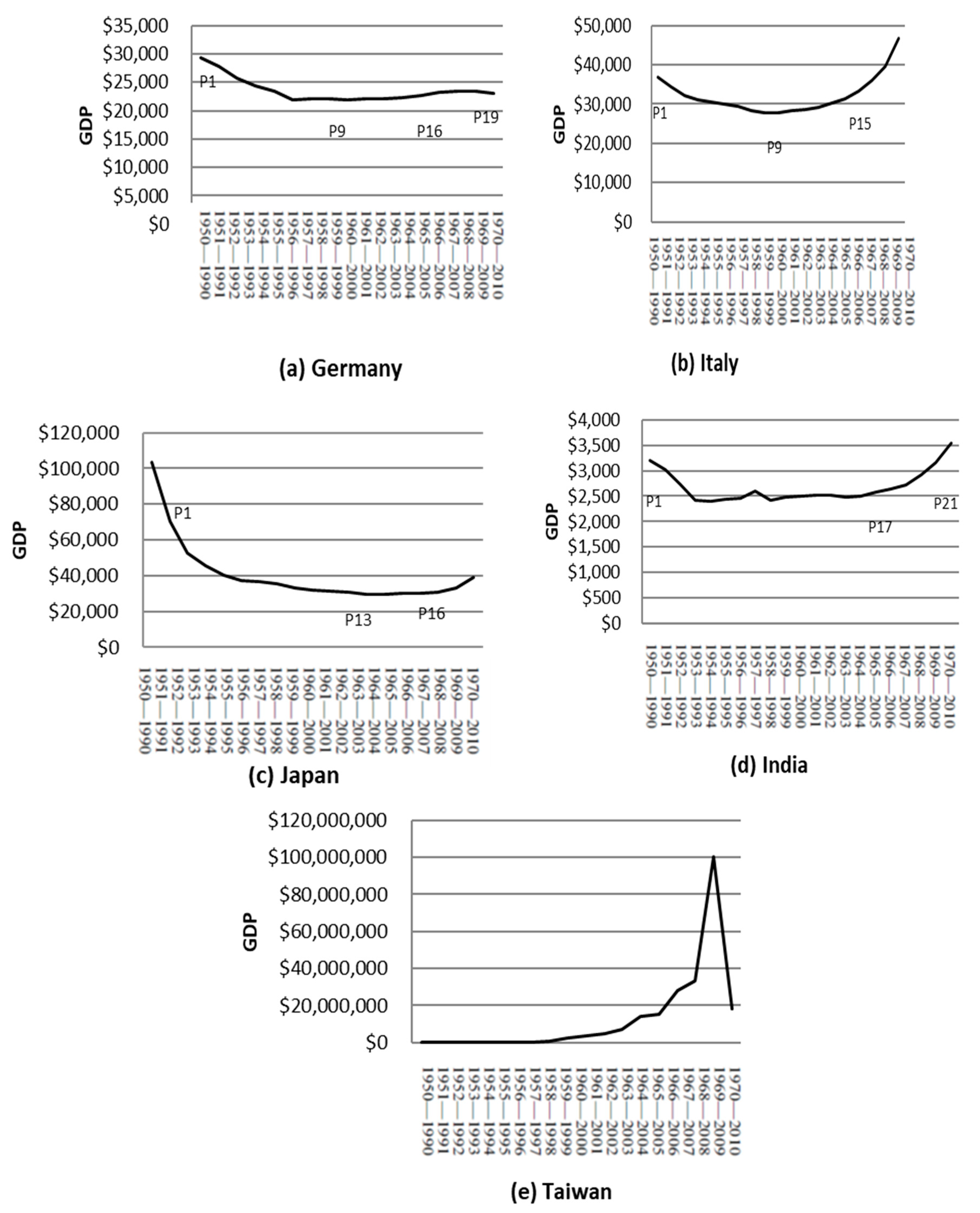
First, presence of the EKC trajectory was demonstrated by the consistently negative signs of the estimated parameters of quadratic income variables in rolling regressions. Second, upon comparing the maximum income value in each country with the corresponding occurring income of the turning points (Table 3, Table 4, Table 5, Table 6 and Table 7), the results revealed that turning points of EKCs were achieved in Germany, Italy, Japan, and India but not Taiwan. Third, the current study demonstrated decreasing trends in income at the turning points of the EKC in the estimated rolling data of three developed countries (Germany, Italy, and Japan) and one developing country (India; Figure 1). The Kyoto Protocol inspired this trend of reduction in CO₂ emissions in these four countries. However, this decrease slowed as the treaty approached its deadline, and no such new commitments have taken effect thus far. Fourth, new industry-based economies such as Taiwan demonstrate a different trajectory. In Taiwan, CO₂ emissions were strongly linked to the increase in income because Taiwan’s economy is highly reliant on export-oriented manufacture industries.

Fifth, it is worthwhile to note that there are notable announcement effects of the treaty, which are affirmed by the evidences that in the years before the treaty was implemented there was an eminent decrease in the estimated income of the turning points. If the income growth sustained, the turning points occurred earlier. The results are consistent with the studies of the government policies [43,44]. Sixth, this study noted that all five countries initially strove to reduce CO₂ emissions during the early period of the treaty but gradually reduced or ceased their efforts as the global economy went into recession and the Kyoto Protocol deadline approached.

The first and second findings confirmed that the decrease in the EKC slope occurred not only after but also before the Kyoto Protocol was enforced by domestic economic policy changes and legislation. This is consistent with the results of Chen [26] and Stefanski [23], that countries aiming to reduce CO₂ emissions and increase income levels have been continuously working towards technological progress to improve energy efficiency which can lower costs and increase economic returns. That is there are long-term common EKC patterns, which is again affirmed by the present study, as well as the studies of Chen [26] and Stefanski [25] for the per capita CO₂ emissions. This study included the two pieces of literature—Stefanski [23], and Chen [24], due to their insight findings to the common EKC patterns which were observed by Chen (2017) for per capita CO₂ emissions in the 21 states in the European Union and over the countries in the world.

These two studies and the present study have indicated that it will have an effect as incentives were applied towards reducing carbon emissions in the respects of energy cost. Global warming is generally attributed to externality. For example, Shafik and Bandopadhyay [27] demonstrated how the externality of climate change had been induced from accumulated atmospheric concentrations of CO₂ emitted from human activity. This is a classic free-rider problem related to CO₂ emissions; no major local costs are associated with the externality of carbon emissions, and all costs in terms of climate change are borne by the rest of the world. They had expressed their concerns regarding the absence of an automatic decrease in incentives embedded in the economy. However, externality induces only the toothless and ineffectual policy in a market-oriented economy and makes us face, as human beings, our own imminent doom. On the contrary, according to the evidences affirmed the EKC patterns found in the present study, together with Chen [26] and Stefanski [25], fossil fuel energy cost embedded in the economy should be taken into consideration, and self-driven incentives of the energy cost in an economy would automatically lead us to a good future. Especially, there are associated incentives continuously led the economy to lower energy cost, conserve energy, improve energy efficiency, progress the technology, and transform to low carbon energy-mix and low carbon economy development.

Although India is a developing country and not bound by the Kyoto Protocol, India’s turning points on the EKC reduced over time, suggesting that (1) developing countries do not always exhibit increasing trends in CO₂ emissions, and (2) an economy relying little on carbon-intensive industries can lower its CO₂ emissions. Rather than economic development stages (which are frequently mentioned in disputes over amendments after enactment of the Kyoto Protocol), green economy and low-carbon development should be the focus of carbon reduction policies.

The CO₂ emission results in Italy indicated that emissions tend to be high in economies dominated by heavy industry. Persistent consumption of fossil fuels enabled early reduction in the turning points of Italy’s EKCs in response to the Kyoto Protocol. Kyoto commitment had reduced the competitiveness of many Kyoto countries and their exports as indicated by Aichele and Felbermayr [37]. It is also induced under large cost adjusting to the austerity policies imposed by the European Union during its economic recessions.

India was the only examined country that relied on industries with low carbon emissions; this enabled it to reduce its CO₂ emissions. Therefore, how an economy adapts to reduce CO₂ emissions rather than its level of economic development or income predominantly affects emission reduction. Moreover, the results of Germany and Japan implied that per capita CO₂ emissions can be reduced through prudent implementation of policies in industrialized countries, even if the total CO₂ emissions remain higher than those in other countries.

The CO₂ emission results in Taiwan suggested that emissions are strongly associated with increases in income and economic development, both of which rely on export-oriented manufacturing. However, irregular turning point changes in recent subperiods, namely P15–P21, indicated that Taiwan’s economy is vulnerable to the global financial crises.

The transition to higher income of the EKC turning points in Italy, Japan, India, and Taiwan indicated a transformation in the reduction trend of CO₂ emissions during the global financial crisis; this is because financial stabilization became the focus over desires to reduce CO₂ emissions. Recovering from the recession became the main priority of many countries, and this hindered efforts to further reduce CO₂ emissions. Restructuring economies to function with low CO₂ emissions reduces risk and damage at both the ends of income increase and CO₂ emission reduction as recession continues to occur. A low-carbon economy involves the pursuit of a long-term vision where income is earned from activities that emit less carbon. Under an economic structure with a low-carbon economy, pursuing income does not hinder reduction of CO₂ emissions.

During the global financial crisis, the Italian government experienced financial problems and struggled to continue its CO₂ emission reduction policies. In Italy, CO₂ emission levels are predicted to remain high because heavy industries dominate Italy’s economy. High fossil fuel-consuming and high CO₂-emitting industries are predominant in Italy.

CO₂ emissions in Japan, which also suffered during the global financial crisis, increased. Only Germany continued to reduce CO₂ emissions, despite the recession. However, in the later years of the recession, the turning points of Germany shifted slightly downward, whereas those of Japan, Italy, and India increased. Recession became an obstacle to reduction of CO₂ emissions.

6. Conclusions

CO₂ emissions—a primary factor of global climate change—mainly originate from fossil fuel combustion. The roles and responsibilities of Kyoto Protocol-bound countries are increasingly debated as further amendments to the protocol are proposed. We investigated time-related changes in CO₂ emission patterns in Germany, Italy, Japan, India, and Taiwan through rolling regression by using turning points on EKCs as indicators. The needs of rolling with a time window to investigate the time trajectory of the turning points in present study had been supports by Ajmi et al. [41].

Regardless of whether countries were bound by the Kyoto Protocol, decreasing trends were observed. In addition to obligating countries to reduce CO₂ emissions, the Kyoto Protocol has led, advocated, and controlled the reduction of CO₂ emissions. However, the period of the first Kyoto Protocol has now ended, and a related amendment is pending. The 24th conference of parties of IPCC was taken place to deal with the implementation of the 2015 Paris Agreement.

Before the signing and ratification of the Kyoto Protocol, Germany and Japan reduced their CO₂ emissions and continued to reduce them in a downward trend at turning points on the rolling EKCs. Before they took effect, the anticipated international policies of the Kyoto Protocol exerted their influence [42], with their announcement effects. Committed countries such as Germany and Japan responded in advance by implementing necessary policy changes.

Prudent design and implementation of CO₂ reduction policies and low-carbon development can reduce CO₂ emissions. Among the five studied countries, only Germany maintained a downward trend in the occurring income of the EKC turning points during the financial crisis. In India, low-carbon economic development has enabled the country to follow EKC patterns and exhibit decreasing trends in the income of the EKC turning points. India is an economy composed of industries with low carbon emissions (e.g., agriculture and computer software design). The empirical evidence confirmed that the structure—rather than the development stage and income—of a country dominates its carbon emissions.

Italy demonstrated a short-term downward trend after ratification of the Kyoto Protocol; however, CO₂ reduction ceased during the global financial crisis because of high emission demands for its heavy industries. In Taiwan, the predominance of export-oriented manufacturing industries caused a sharp increase in CO₂ emissions following economic development. During the global financial crisis, Taiwan’s vulnerable economy required stable income and increased per capita CO₂ emissions. The results of the present study suggested that rather than focusing on the stage of economic development, countries should restructure their economies to enable them to reduce their carbon dependency. Prudent reduction policies and low-carbon development can effectively reduce CO₂ emissions.

Thus, the Kyoto Protocol can promote reduction of CO₂ emissions in Annex I countries.

Limitations of the present study and recommendations for the future study are made here. First, we selected only data from 1950–2010, and thus we were unable to investigate the effects of reduction in CO₂ emissions after the first commitment period had ended. Second, some countries participated in the Kyoto Protocol’s first commitment period but did not adopt new targets in the subsequent period. Whether such countries exhibited unconducive trends in reduction of CO₂ emissions remains unclear. These topics warrant additional research. Third, in this study, we investigated trends in CO₂ emissions by observing the EKCs of five countries and by rolling data forward to alter the turning points. This study evaluated the overall effects of Kyoto Protocol-related policies in five countries with differential responsibilities throughout the study period. Distinguishing individual effects from a single policy was not in the scope of this study. Fourth, Lantz and Feng [60] suggested that total or per capita data analysis can lead to variations in turning points and the results can change according to the estimation method used. The results and inferences of this study were based on per capita CO₂ emissions and per capita income and the model specification adopted in this study.

It is worthwhile to note the argument about statistical significance of the turning points. By including energy mix and other variables in the study on OECD countries, Richmond and Kaufmann [14] had found statistical support for a turning point would be eliminated and suggested invalidity of applying turning points to be an accurate policy reference. As reviewed in the section of literature, the argument for the statistical support of the EKC turning points is valid only for a panel study on countries with heterogeneity in their economic structure, energy mix, climate policy, like the empirical study provided by Richmond and Kaufmann [14,15]. In the studies on a group of the homogeneity countries and/or on single countries, EKC turning points seems good to indicate the time transitions of CO₂ emissions. However, thorough justification is suggested to be left to econometrists in their future study.

Fifth, regarding the time length of the fixed-window in a rolling regression analysis, there is no clear selection rule for (the observation number of the sub-period) in the textbook of a rolling regression wrote by Zivot and Wang [17]. Relevant literature [17,18,19] had indicated that the stability of a model or the economic structure revealed through data is typically evaluated using the model’s predictive ability. Recent econometric research [61] had proposed the criterion in selection of rolling window based on predicted ability. However, this study did not adopt this criterion and future research in the related issues can further consider the criterion.

References

1. National Oceanic Atmospheric Administration. NOAA Climate Report. Available online: http://www.noaanews.noaa.gov/ (accessed on 10 June 2012).
2. Intergovernmental Panel on Climate Change. Available online: http://www.ipcc.ch/ (accessed on 10 June 2012).[Green Version]
3. UNFCCC. Text of the Kyoto Protocol. Available online: http://unfccc.int/essential_background/convention/background.php (accessed on 10 June 2012).
4. Grunewald, N.; Klasen, S.; Martínez-Zarzoso, I.; Muris, C. Income Inequality and Carbon Emissions; Courant Research Centre: Poverty, Equity and Growth—Discussion Papers, No. 92; Courant Research Centre Poverty, Equity and Growth, Göttingen University: Göttingen, Germany, 2011. [Google Scholar]
5. United Nations Environment Programme. Doha Climate Conference Gateway. Available online: http://www.unep.org/newscentre/default.aspx?DocumentID=2700&ArticleID=9353 (accessed on 15 December 2012).
6. Huang, M.W.; Lee, G.W.M.; Wu, C.C. GHG Emissions, GDP Growth and the Kyoto Protocol: A Revisit of Environmental Kuznets Curve Hypothesis. J. Energy Policy 2008, 36, 239–247. [Google Scholar] [CrossRef]
7. UNFCCC. What Is the Paris Agreement? Available online: https://unfccc.int/process-and-meetings/the-paris-agreement/what-is-the-paris-agreement (accessed on 15 January 2019).
8. UNFCCC. Katowice Climate Change Conference—December 2018. Available online: https://unfccc.int/katowice (accessed on 15 January 2019).
9. European Climate Change Programme. Climate Action. Available online: https://ec.europa.eu/clima/index_en (accessed on 18 January 2019).
10. Eurostat. Industry Trade and Services. Available online: https://ec.europa.eu/eurostat/web/euro-indicators/industry-trade-and-services (accessed on 12 January 2019).
11. Müller-Fürstenberger, G.; Wagner, M. Exploring the Carbon Kuznets Hypothesis; Discussion Paper; University of Bern, Department of Economics: Bern, Switzerland, 2004. [Google Scholar]
12. Müller-Fürstenberger, G.; Wagner, M. Exploring the Environmental Kuznets Hypothesis: Theoretical and Econometric Problems. Ecol. Econ. 2007, 62, 648–660. [Google Scholar] [CrossRef]
13. Vollebergh, H.R.J.; Melenberg, B.; Dijkgraaf, E. Identifying Reduced-form Relations with Panel Data: The Case of Pollution and Income. J. Environ. Econ. Manag. 2009, 58, 27–42. [Google Scholar] [CrossRef]
14. Richmond, A.K.; Kaufmann, R.K. Is There a Turning Point in The Relationship between Income and Energy Use and/or Carbon Emissions? Ecol. Econ. 2006, 56, 176–189. [Google Scholar] [CrossRef]
15. Richmond, A.K.; Kaufmann, R.K. Energy Prices and Turning Points: The Relationship between Income and Energy Use/Carbon Emissions. Energy J. 2006, 27, 157–180. [Google Scholar] [CrossRef]
16. Coondoo, D.; Dinda, S. Carbon Dioxide Emission and Income: A Temporal Analysis of Cross-country Distributional Patterns. Ecol. Econ. 2008, 65, 375–385. [Google Scholar] [CrossRef]
17. Zivot, E.; Wang, J. Chapter 9 Rolling analysis of time series. In Modeling Financial Time Series with S-Plus, 2nd ed.; Springer: New York, NY, USA, 2006. [Google Scholar]
18. Diebold, F.X.; Mariano, R.S. Comparing Predictive Accuracy. J. Bus. Econ. Stat. 1995, 13, 253–263. [Google Scholar] [Green Version]
19. Diebold, F.X. Comparing Predictive Accuracy, Twenty Years Later: A Personal Perspective on the Use and Abuse of Diebold-Mariano Tests. J. Bus. Econ. Stat. 2015, 33, 1–9. [Google Scholar] [CrossRef]
20. Grossman, G.; Krueger, A. Environmental Impacts of a North American Free Trade Agreement; National Bureau of Economics Research Working Paper, 3194; NBER: Cambridge, MA, USA, 1991. [Google Scholar]
21. Grossman, G.; Krueger, A. Economic Environment and the Economic Growth. Q. J. Econ. 1995, 110, 353–377. [Google Scholar] [CrossRef]
22. Shafik, N. Economic Development and Environmental Quality: An Econometric Analysis. Oxf. Econ. Pap. 1994, 46, 757–773. [Google Scholar] [CrossRef]
23. De Bruyn, S.M.; van den Bergh, J.C.J.M.; Opschoor, J.B. Economic Growth and Emissions: Reconsidering the Empirical Basis of Environmental Kuznets Curves. J. Ecol. Econ. 1998, 25, 161–175. [Google Scholar] [CrossRef]
24. Friedl, B.; Getzner, M. Determinants of CO2 Emissions in a Small Open Economy. J. Ecol. Econ. 2003, 45, 133–148. [Google Scholar] [CrossRef]
25. Stefanski, R. On the Mechanics of the “Green Solow Model”, No.47; OxCarre Research Paper: Oxford, UK, 2013. [Google Scholar]
26. Chen, W.J. Is the Green Solow Model Valid for CO2 Emissions in the European Union? Environ. Resour. Econ. 2017, 67, 23–45. [Google Scholar] [CrossRef]
27. Shafik, N.; Bandyopadhyay, S. Economic growth and environmental resources. J. Environ. Econ. Manag. 1992, 4, 1–24. [Google Scholar]
28. Cole, M.A. Development, Trade, and The Environment: How Robust is the Environmental Kuznets Curve? J. Environ. Dev. Econ. 2003, 8, 557–580. [Google Scholar] [CrossRef]
29. Park, S.; Lee, Y. Regional Model of EKC for Air Pollution: Evidence from the Republic of Korea. J. Energy Policy 2011, 39, 5840–5849. [Google Scholar] [CrossRef]
30. Esteve, V.; Tamarit, C. Threshold Cointegration and Nonlinear Adjustment between CO2 an Income: The Environmental Kuznets Curve in Spain, 1857–2007. J. Energy Econ. 2012, 34, 2148–2156. [Google Scholar] [CrossRef]
31. Roberts, J.T.; Grimes, P.E. Carbon Intensity and Economic Development 1962–91: A Brief Exploration of the Environmental Kuznets Curve. World Dev. 1997, 25, 191–198. [Google Scholar] [CrossRef]
32. Antle, J.M.; Heidebrink, R. Environment and Development: Theory and International Evidence. Econ. Dev. Cult. Chang. 1995, 43, 604–625. [Google Scholar] [CrossRef]
33. Xepapadeas, A. Economic growth and the environment. Handb. Environ. Econ. 2005, 3, 1220–1271. [Google Scholar]
34. Markandya, A.; Colub, A.; Pedroso-Galinato, S. Empirical Analysis of National Income and SO2 Emissions in Selected European Parties. J. Environ. Resour. Econ. 2006, 35, 221–257. [Google Scholar] [CrossRef]
35. Panayotou, T. Economic Growth and the Environment; Spring Seminar of the United Nations Economic Commission for Europe: Geneva, Switzerland, 2003. [Google Scholar]
36. Aichele, R.; Felbermayr, G. Kyoto and Carbon Leakage: An Empirical Analysis of the Carbon Content of Bilateral Trade. Rev. Econ. Stat. 2014, 97, 104–115. [Google Scholar] [CrossRef]
37. Aichele, R.; Felbermayr, G. Estimating the Effects of Kyoto on Bilateral Trade Flows Using Matching Econometrics. World Econ. 2013, 36, 303–330. [Google Scholar] [CrossRef] [Green Version]
38. Aichele, R.; Felbermayr, G. The Effect of the Kyoto Protocol on Carbon Emissions. J. Policy Anal. Manag. 2013, 32, 731–757. [Google Scholar] [CrossRef]
39. Aichele, R.; Felbermayr, G. Kyoto and the Carbon Footprint of Nations. J. Environ. Econ. Manag. 2012, 63, 336–354. [Google Scholar] [CrossRef]
40. Baghdadi, L.; Martinez-Zarzoso, I.; Zitouna, H. Are RTA agreements with environmental provisions reducing emissions? J. Int. Econ. 2013, 90, 378–390. [Google Scholar] [CrossRef] [Green Version]
41. Ajmi, A.N.; Hammoudeh, S.; Nguyen, D.K.; Sato, J.R. On the Relationships between CO2 emissions, energy Consumption and Income: The Importance of Time Variation. Energy Econ. 2015, 49, 629–638. [Google Scholar] [CrossRef]
42. Chen, J.H.; Lai, C.C.; Shieh, J.Y. Anticipated Environmental Policy and Transitional Dynamics in an Endogenous Growth Model. Environ. Resour. Econ. 2003, 25, 233–254. [Google Scholar] [CrossRef]
43. Barker, T.; Ekins, P.; Foxon, T. Macroeconomic effects of efficiency policies for energy-intensive industries: The case of the UK Climate Change Agreements, 2000–2010. Energy Econ. 2007, 29, 760–778. [Google Scholar] [CrossRef]
44. Smulders, S.; Tsur, Y.; Zemel, A. Announcing Climate Policy: Can a Green Paradox Arise without Scarcity? J. Environ. Econ. Manag. 2012, 64, 364–376. [Google Scholar] [CrossRef]
45. Galeotti, M.; Lanza, A.; Pauli, F. Reassesing the Environmental Kuznets Curve for CO2 emissions: A Robustness Exercise. J. Ecol. Econ. 2006, 57, 152–163. [Google Scholar] [CrossRef]
46. CDIAC. Retrieve Carbon Dioxide Emission Data from the Carbon Dioxide Information Analysis Center, CDIAC. Available online: http://cdiac.ornl.gov/ (accessed on 1 May 2012).
47. Kumazawa, R.; Callaghan, M.S. The effect of the Kyoto Protocol on carbon dioxide emissions. J. Econ. Financ. 2012, 36, 201–210. [Google Scholar] [CrossRef]
48. Holtz-Eakin, D.; Selden, T.M. Stoking the Fire? CO2 Emission and Economic Growth. J. Public Econ. 1995, 57, 85–101. [Google Scholar] [CrossRef]
49. Perman, R.; Stern, D.I. Evidence from Panel Unit Root and Cointegration Tests That the Environmental Kuznets Curve Does Not Exist. Aust. J. Agric. Resour. Econ. 2003, 47, 325–347. [Google Scholar] [CrossRef]
50. Lee, C.C.; Lee, J.D. Income and CO2 Emissions: Evidence from Panel Unit Root and Cointegration Tests. J. Energy Policy 2009, 37, 413–423. [Google Scholar] [CrossRef]
51. Granger, C.W.J.; Newbold, P. Spurious Regression in Econometrics. J. Econom. 1974, 2, 111–120. [Google Scholar] [CrossRef]
52. Kwiatkowski, D.; Phillips, P.C.; Schmidt, P.; Shin, Y. Testing the Null Hypothesis of Stationarity against the Alternative of a Unit Root. J. Econom. 1992, 54, 159–178. [Google Scholar] [CrossRef]
53. Johansen, S. Statistical Analysis of Cointegrating Vectors. J. Econ. Dyn. Control 1988, 12, 231–254. [Google Scholar] [CrossRef]
54. Johansen, S.; Juselius, K. Maximum Likelihood Estimation and Inference on Cointegration, with Applications to the Demand for Money. Oxf. Bull. Econ. Stat. 1990, 52, 169–210. [Google Scholar] [CrossRef]
55. Albrecht, J.; François, D.; Schoors, K. A Shapley Decomposition of Carbon Emissions without Residuals. Energy Policy 2002, 30, 727–736. [Google Scholar] [CrossRef]
56. Statista., Refinery Capacities in Selected Countries in Europe in 2017 (in 1000 Barrels Daily), Energy and Environmental Service, the Statistic Patrol. Available online: https://www.statista.com/statistics/332198/refinery-capacities-in-europe-by-country/ (accessed on 11 August 2018).
57. European Commission. European Policy of Climate. Available online: http://ec.europa.eu/index_en.htm (accessed on 15 September 2012).
58. Jaunky, V.C. The CO2 Emissions-Income Nexus: Evidence form Rich Parties. J. Energy Policy 2011, 39, 1228–1240. [Google Scholar] [CrossRef]
59. Neter, J.; Kutner, M.H.; Nachtsheim, C.J.; Wasserman, W. Applied Linear Statistical Models, 4th ed.; Irwin: Chicago, IL, USA, 1996; p. 1321. [Google Scholar]
60. Lantz, V.; Feng, Q. Assessing Income, Population, and Technology Impacts on CO2 Emissions in Canada: Where’s the EKC? Ecol. Econ. 2006, 57, 229–238. [Google Scholar] [CrossRef]
61. Inoue, A.; Jin, L.; Rossi, B. Rolling Window Selection for Out-of-sample Forecasting with Time-varying Parameters. J. Econom. 2017, 196, 55–67. [Google Scholar] [CrossRef]
Figure 1. Transition of environmental Kuznets curve (EKC) turning points for the five single parties. (Annual GDP per capita measured in USD. The scales in vertical axis are different).
Sustainability 11 00744 g001