Measuring Risk Allocation of Tax Burden for Small and Micro Enterprises


Abstract
:1. Introduction
2. Literature Review
3. Data and Model
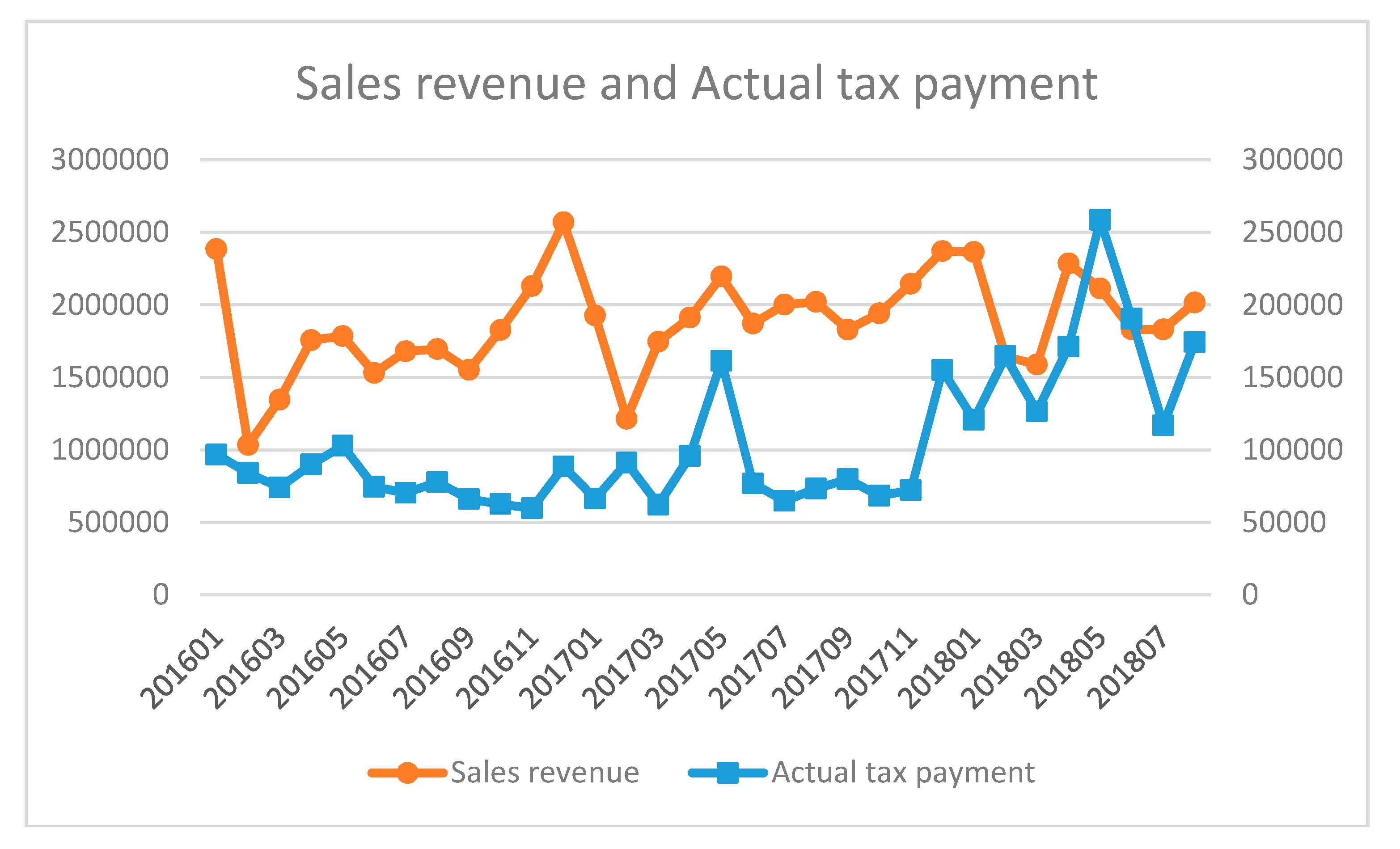
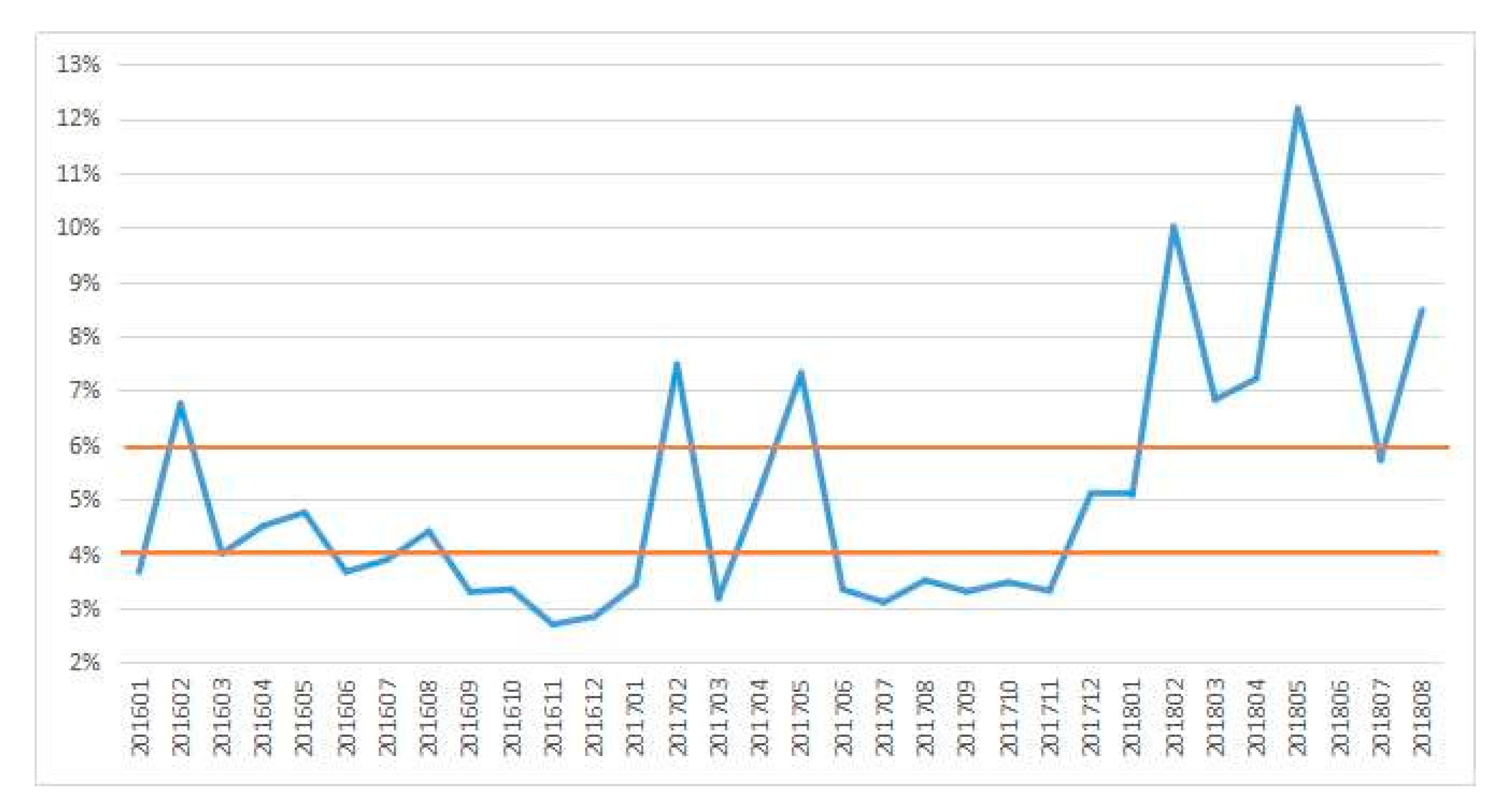
3.1. Data Description
3.2. Question
3.3. Initial Model
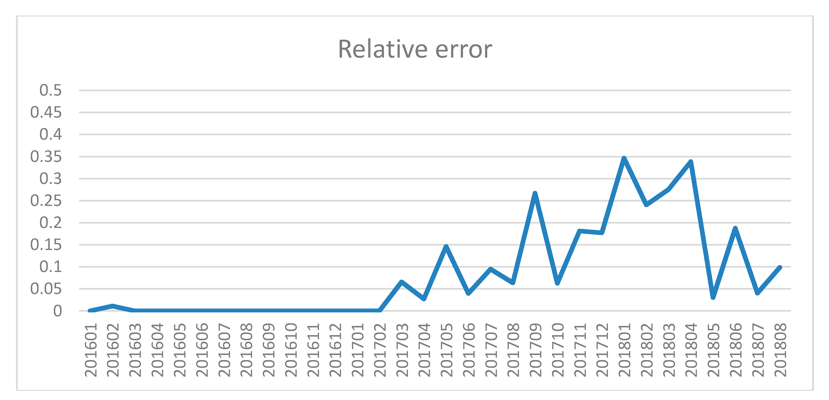
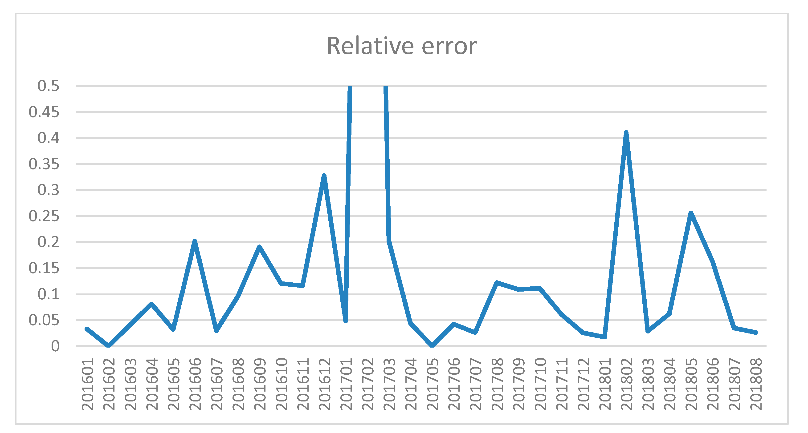
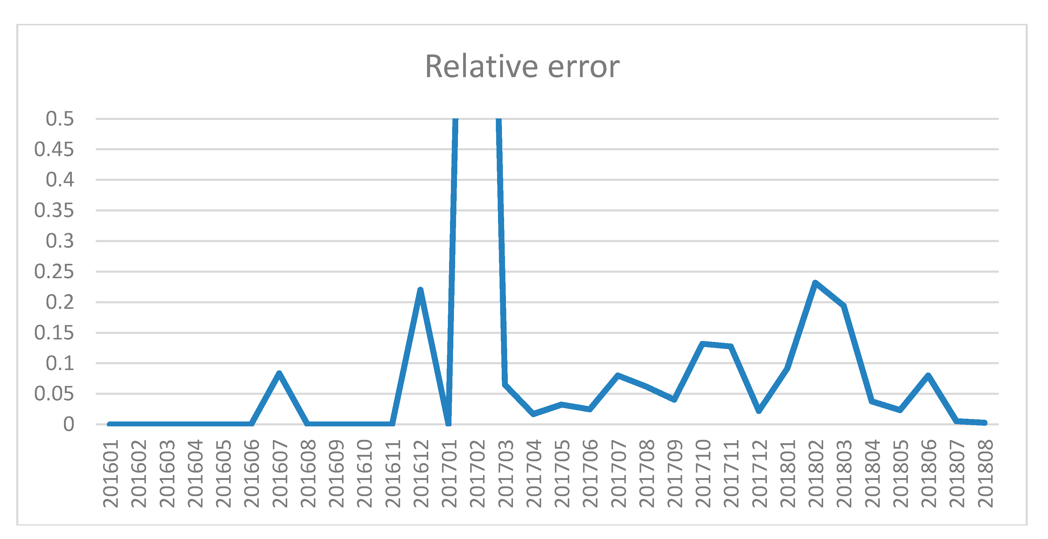
3.4. Error Test
4. Measuring Risk Allocation of the Tax Burden
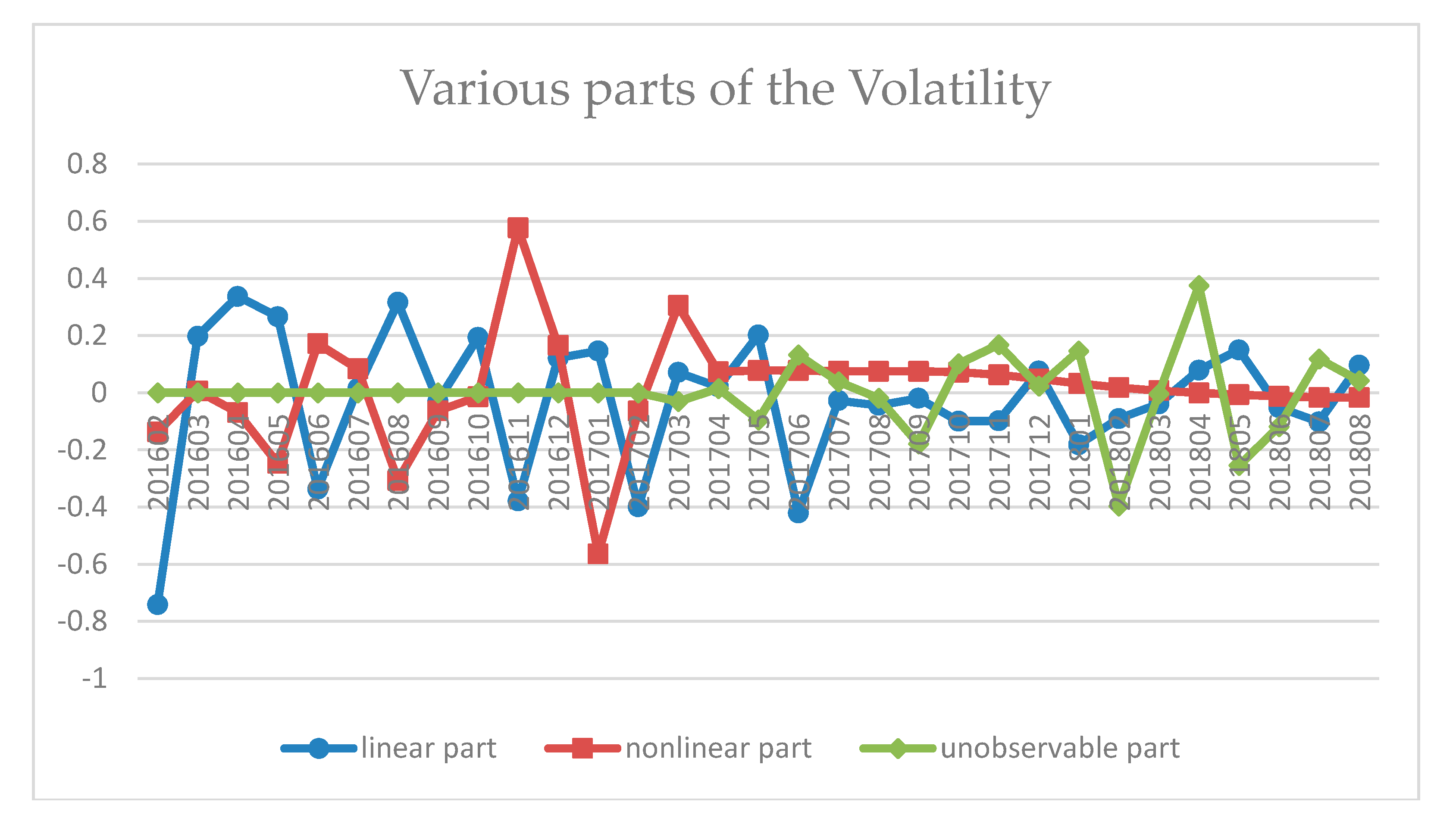
4.1. Volatility or Trend
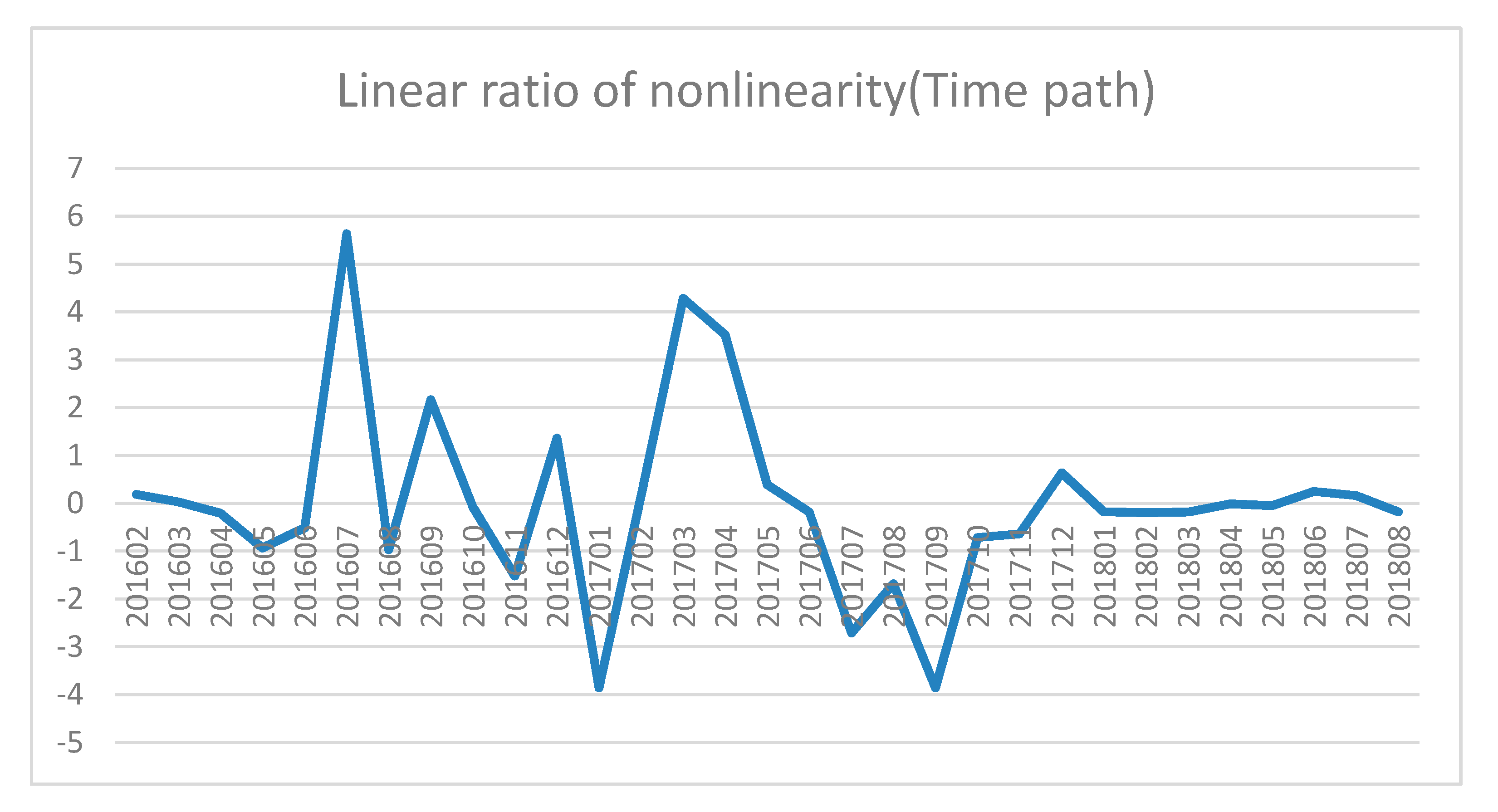
4.2. Tax Burden along the Time Path
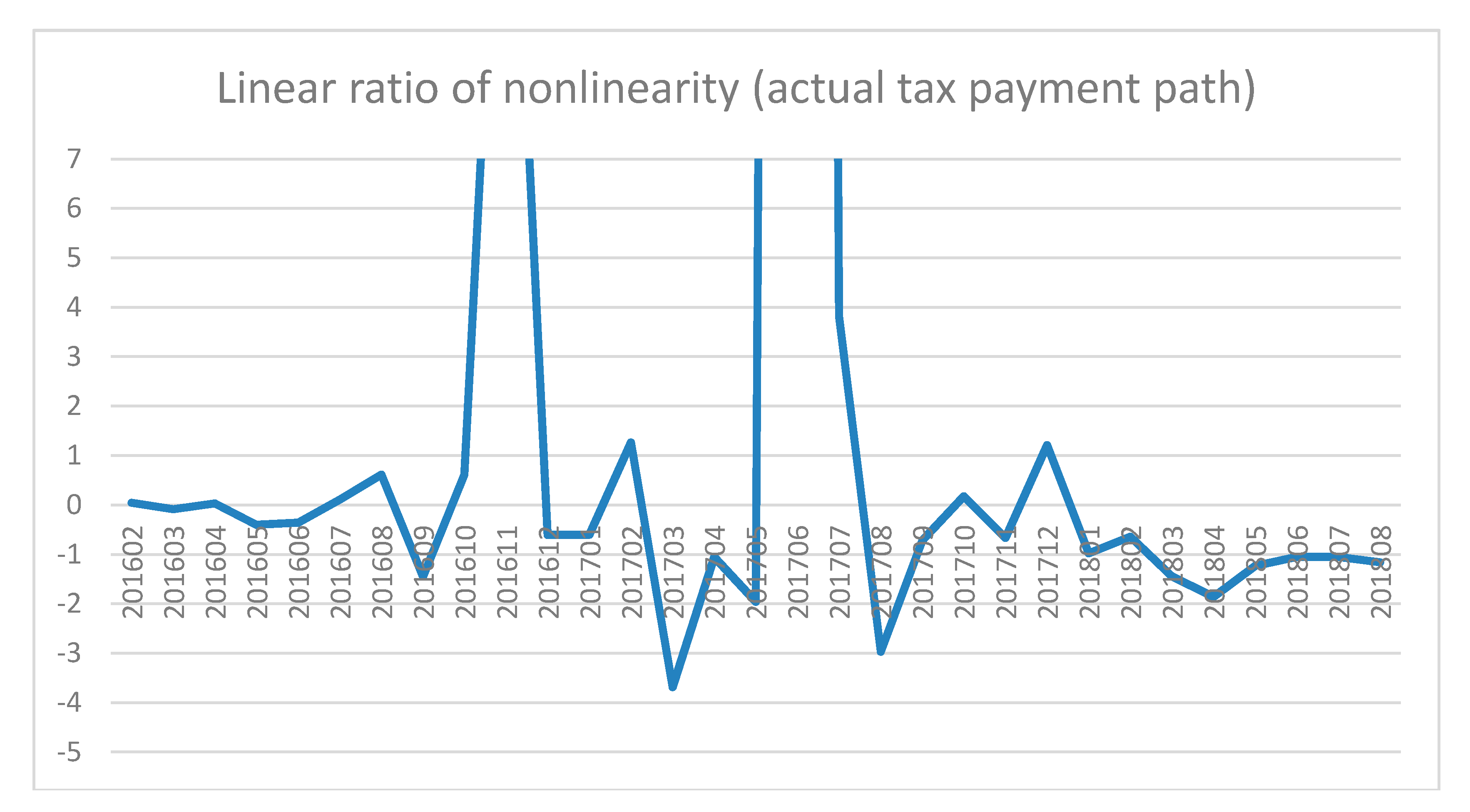
4.3. Tax Burden along Actual Tax Payment or Credit Path
5. Improving Tax Risk Allocation
5.1 Model Description
5.2. Results and Discussions
5.2.1. Outliers Improvement (Full Sample Analysis)
5.2.2. Classified Enterprise Analysis
The First Category of Enterprises
The Second Category of Enterprises
The Third Category of Enterprises
5.3. Discussions
6. Conclusions
Author Contributions
Acknowledgments
Conflicts of Interest
References
- Jiang, J.Q. Problems and Countermeasures in the Operation of Government-Supported Funds. Priv. Sci. Technol. Phase 2014, 10, 207–208. [Google Scholar]
- World Trade Report 2016—Levelling the Trading Field for SMEs. 2016. Available online: https://www.wto.org/english/res_e/booksp_e/world_trade_report16_e.pdf (accessed on 12 December 2018).
- Mason, M.K. What Causes Small Businesses to Fail; MKM Research Publishers: Agnantero Karditsa, Greece, 2009; Available online: http://www.moyak.com/papers/small-business-failure.html (accessed on 1 December 2018).
- Commerce, U.D.O. The competitiveness and innovative capacity of the United States. Us Dep. Commer. 2012, 1, 160. [Google Scholar]
- Mnenwa, R.; Maliti, E. The Role of Small Businesses in Poverty Alleviation: The Case of Dar es Salaam, Tanzania. 2008. Available online: https://www.africaportal.org/publications/the-role-of-small-businesses-in-poverty-alleviation-the-case-of-dar-es-salaam-tanzania/ (accessed on 11 December 2018).
- Dhaliwal, D.S.; Gaertner, F.B.; Seung, H.; Trezevant, R. Historical cost, inflation, and the US corporate tax burden. J. Account. Public Policy 2015, 34, 467–489. [Google Scholar] [CrossRef]
- Fuest, C.; Peichl, A.; Siegloch, S. Do higher corporate taxes reduce wages? Micro evidence from Germany. Am. Econ. Rev. 2018, 108, 393–418. [Google Scholar] [CrossRef]
- Auerbach, A.J. Measuring the Effects of Corporate Tax Cuts. J. Econ. Perspect. 2018, 32, 97–120. [Google Scholar] [CrossRef]
- Chen, D.; Qi, S.; Schlagenhauf, D. Corporate income tax, legal form of organization, and employment. Am. Econ. J. Macroecon. 2018, 10, 270–304. [Google Scholar] [CrossRef]
- Luo, S.; Zhang, Y.; Zhou, G. Financial Structure and Financing Constraints: Evidence on Small-and Medium-Sized Enterprises in China. Sustainability 2018, 10, 1774. [Google Scholar] [CrossRef]
- Pizzacalla, M. Global SME tax policy conundrum. Aust. Tax Forum 2008, 23, 49. [Google Scholar]
- Greenhalgh, C.; Rogers, M. Innovation, Intellectual Property, and Economic Growth; Princeton University Press: Princeton, NJ, USA, 2010. [Google Scholar]
- Xu, B.; Xiao, Y.; Rahman, M.U. Enterprise level cluster innovation with policy design. Entrep. Reg. Dev. 2018, 31, 46–61. [Google Scholar] [CrossRef]
- Atkinson, R.D. Expanding the R&E tax credit to drive innovation, competitiveness and prosperity. J. Technol. Transf. 2007, 32, 617–628. [Google Scholar]
- Burlamaqui, L.; Cimoli, M. Industrial policy and IPR: A knowledge governance approach. Intellect. Prop. Rights: Leg. Econ. Chall. Dev. 2014, 2014, 477–502. [Google Scholar]
- Grubert, H.; Altshuler, R. Shifting the burden of taxation from the corporate to the personal level and getting the corporate tax rate down to 15 percent. In Annual Conference on Taxation and Minutes of the Annual Meeting of the National Tax Association; National Tax Association: Columbus, OH, USA, 2015; pp. 1–53. [Google Scholar]
- Hines, J.R., Jr. Business Tax Burdens and Tax Reform. Brook. Pap. Econ. Act. 2017, 2017, 449–477. [Google Scholar] [CrossRef]
- Salaudeen, Y.M.; Atoyebi, T.A. Tax Burden Implication of Tax Reform. Open J. Bus. Manag. 2018, 6, 761. [Google Scholar] [CrossRef]
- Czékus, Á. The Impact of Reducing the Corporate Income Tax Rate on the State Aid Practices of EU Member States (2000 to 2015). Public Financ. Q. 2018, 63, 216–234. [Google Scholar]
- Fang, H.; Yu, L.; Hong, Y.; Zhang, J. Tax Burden, Regulations and the Development of the Service Sector. Emerg. Mark. Financ. Trade 2019, 55, 477–495. [Google Scholar] [CrossRef]
- Ye, J.; Guo, X.; Luo, D.; Jin, X. The Heterogeneous Tax Burden: Evidence from Firm-Level Data in China. Singap. Econ. Rev. 2018, 63, 1003–1035. [Google Scholar] [CrossRef]
- Cai, J.; Chen, X.; Dai, M. Portfolio selection with capital gains tax, recursive utility, and regime switching. Manag. Sci. 2017, 64, 2308–2324. [Google Scholar] [CrossRef]
- Hall, P.; Li, Q.; Racine, J.S. Nonparametric estimation of regression functions in the presence of irrelevant regressors. Rev. Econ. Stat. 2007, 89, 784–789. [Google Scholar] [CrossRef]
- Zhu, S. Interpretation of the Law of the People’s Republic of China on Tax Collection and Administration; Financial and Economic Publishing House: Beijing, China, 2001. [Google Scholar]
- Meiling, X. Tax burden, repayment ability and corporate financial performance. Commun. Financ. Account. 2018, 33, 118–123. [Google Scholar]
- Liang, B.; Zhao, Y. Problems and Suggestions on Basic Management of Small and Medium-sized Enterprises. Metall. Financ. Account. 2004, 23, 44–45. [Google Scholar]


| Variable | Symbolic Representation | Variable | Symbolic Representation |
|---|---|---|---|
| Sales revenue | Y | Credit period | |
| Taxable amount | Actual tax payment | ||
| Used credit line | Credit line | ||
| The total wages of employees | - | - |
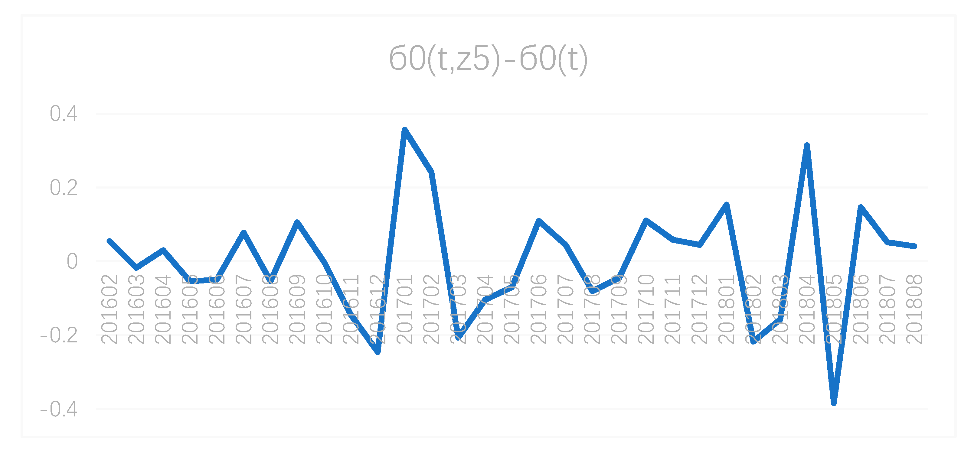
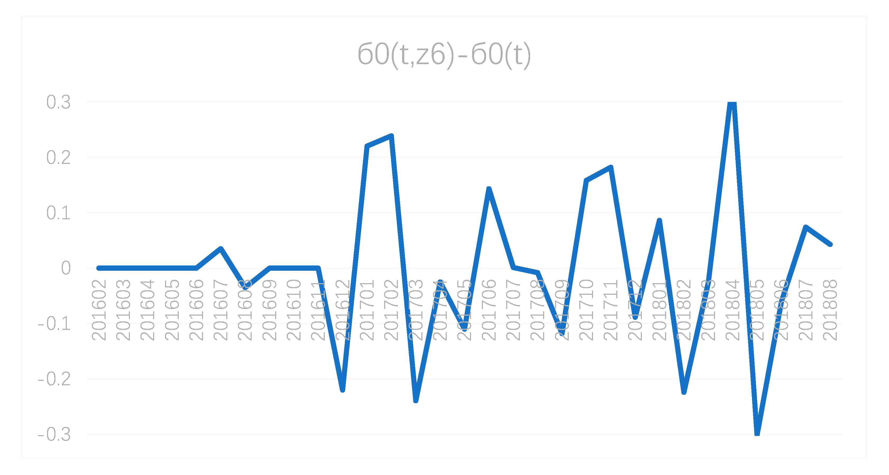
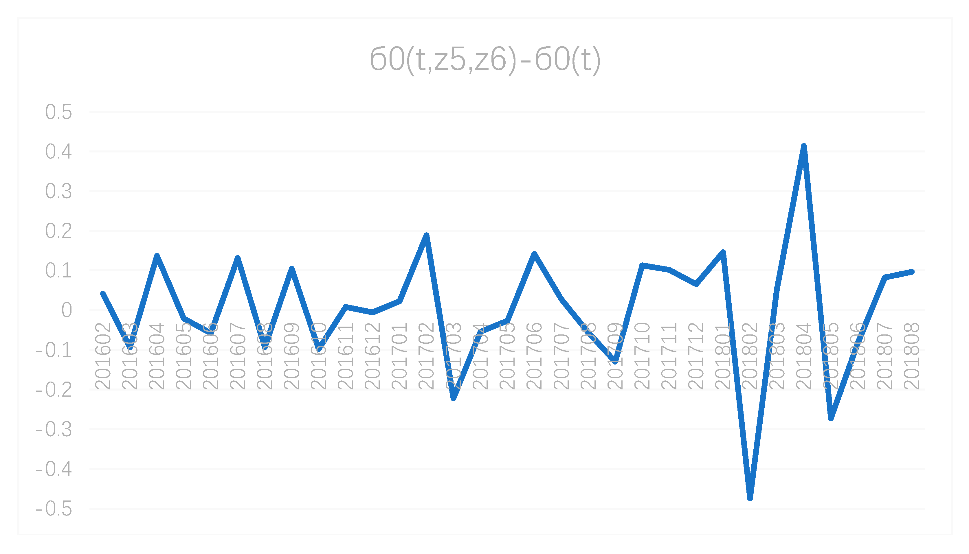
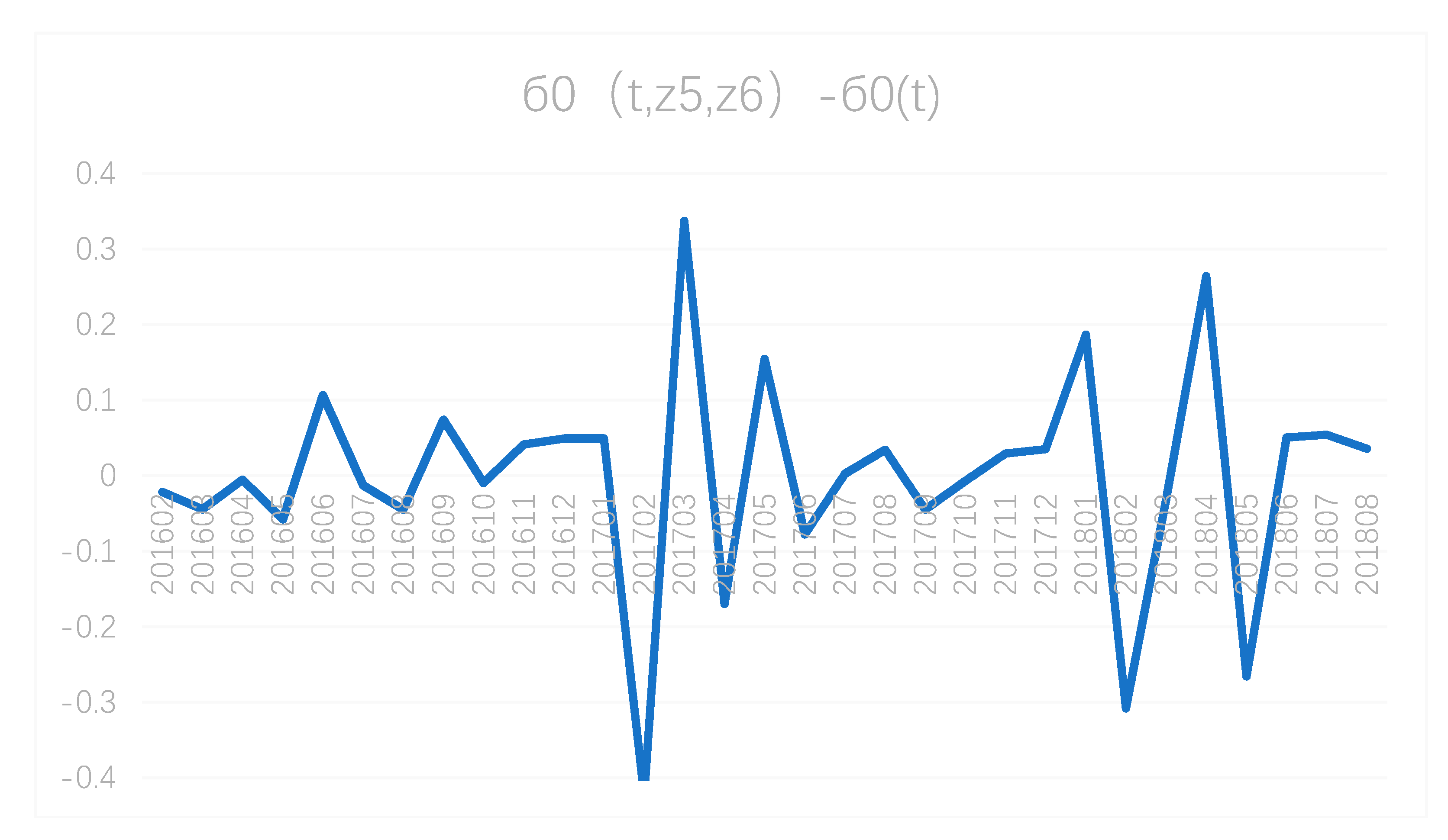
| Path−Benchmark | 201612 | 201703 | 201802 | 201805 |
|---|---|---|---|---|
| −0.245 | −0.206 | −0.217 | −0.384 | |
| −0.220 | −0.240 | −0.224 | −0.302 | |
| −0.006 | −0.222 | −0.474 | −0.272 |
| t | Before Improvement | Improved |
|---|---|---|
| 201802 | 10.01% | 5.32% |
| 201805 | 12.18% | 9.52% |
| t | Before Improvement | Improved |
|---|---|---|
| 201802 | 8.27% | 4.69% |
| 201805 | 9.26% | 6.72% |
| t | Before Improvement | Improved |
|---|---|---|
| 201802 | 12.70% | 5.98% |
© 2019 by the authors. Licensee MDPI, Basel, Switzerland. This article is an open access article distributed under the terms and conditions of the Creative Commons Attribution (CC BY) license (http://creativecommons.org/licenses/by/4.0/).
Share and Cite
Xu, B.; Li, L.; Liang, Y.; Rahman, M.U. Measuring Risk Allocation of Tax Burden for Small and Micro Enterprises. Sustainability 2019, 11, 741. https://doi.org/10.3390/su11030741
Xu B, Li L, Liang Y, Rahman MU. Measuring Risk Allocation of Tax Burden for Small and Micro Enterprises. Sustainability. 2019; 11(3):741. https://doi.org/10.3390/su11030741
Chicago/Turabian StyleXu, Bing, Lili Li, Yan Liang, and Mohib Ur Rahman. 2019. "Measuring Risk Allocation of Tax Burden for Small and Micro Enterprises" Sustainability 11, no. 3: 741. https://doi.org/10.3390/su11030741
APA StyleXu, B., Li, L., Liang, Y., & Rahman, M. U. (2019). Measuring Risk Allocation of Tax Burden for Small and Micro Enterprises. Sustainability, 11(3), 741. https://doi.org/10.3390/su11030741