Article

Social Capital and Adoption of Alternative Conservation Agricultural Practices in South-Western Nigeria

by
Seyi Olalekan Olawuyi
* and
Abbyssinia Mushunje
Department of Agricultural Economics and Extension, University of Fort Hare, P/Bag X1314, Alice 5700, Eastern Cape Province, South Africa
*
Author to whom correspondence should be addressed.
Sustainability 2019, 11(3), 716; https://doi.org/10.3390/su11030716
Submission received: 29 September 2018 / Revised: 20 November 2018 / Accepted: 26 November 2018 / Published: 30 January 2019

Abstract

:
The major concern of most African countries, including Nigeria, in recent times is how to increase food production because of food insecurity issues, which by extension, is a major contributing factor to the prevalence of poverty. Therefore, adoption of conservation agricultural practices is regarded as a pathway to drive the achievement of food and nutrition security, as well as the needed optimal performance in the agri-food sector. Reportedly, scaling up of the limited adoption of these practices could be facilitated through kinship ties, peer influence, and social networks that govern mutual interactions among individuals; therefore, this motivated the study. Using cross-sectional data obtained from 350 sample units selected from South-Western Nigeria through a multistage sampling technique, this study applied descriptive statistical tools and cross-tabulation techniques to profile the sampled subjects while count outcome models were used to investigate the factors driving counts of conservative agriculture (CA) adoption. Similarly, a marginal treatment effects (MTEs) model (parametric approach) using local IV estimator was applied to examine the effects of CA adoption on the outcome (log of farmers’ farm income). Additionally, appropriate measures of fit tests statistics were used to test the reliabilities of the fitted models. Findings revealed that farmers’ years of farming experience (p < 0.1), frequency of extension visits (p < 0.05), and social capital viz-a-viz density of social group memberships (p < 0.05) significantly determined the count of CA practices adopted with varying degrees by smallholder farmers. Although, social capital expressed in terms of membership of occupational group and diversity of social group members also had a positive influence on the count of CA practices adopted but not significant owing largely to the “information gaps” about agricultural technologies in the study area. However, the statistical tests of the MTEs indicated that the treatment effects differed significantly across the covariates and it also varied significantly with unobserved heterogeneity. The policy relevant treatment effect estimates also revealed that different policy scenarios could increase or decrease CA adoption, depending on which individuals it induces to attract the expected spread and exposure.

1. Background Information

Sustainable economic growth and development in a developing economy like Nigeria is achievable through the agricultural sector and its sub-sectors which are concentrated in rural areas, home to the majority (about 75%) of the households practicing farming for family sustenance and/or earning income from the sales of agricultural products [1]. In addition to the persistent use of traditional farming practices, these rural farming households cultivate crop varieties that are low-yielding on small and scattered farmland holdings (smallholder farmers). This act depletes the soil organic matter with devastating consequences on production output, income generation as well as the ecosystem. Similarly, non-access to agricultural credit and limited technical know-how are part of the challenges facing the development of farming activities in sub-Saharan Africa, including Nigeria [2]. These challenges call for holistic interventions that are sustainable, promote a safe environment, and ultimately increase production output. Thus, a practice with zero environmental and human hazards which have literatures converging [3,4,5,6,7,8,9,10,11] on its capability to use renewable local farm resources for sustainable and increased production output is called conservative agriculture (CA).
Generally, CA is regarded as a resource saving agricultural practice that can help farmers simultaneously harvest high yield and conserve the environment [12]. Besides, the water retention characteristic of CA makes it suitable in water deficient farming areas. The basic CA principles include the following practices: minimum soil disturbance, the use of crop biomass for permanent soil cover, and sequential rotation practice for different unrelated crops; all these can potentially strengthen farmers’ resilience to climate change and enhance the sustainability of agro-ecosystems [13,14,15,16]. The diagrammatic view of these three CA packages required for full adoption, according to these authors is shown in Figure 1.
Equally, the major concern of most African countries (including Nigeria) in recent times is how to increase food production [18]. Meanwhile, rural food insecurity is a major contributing factor to widespread poverty in Africa, and Nigeria is no exception, where most farmers are peasants. Therefore, CA is regarded as a panacea to achieving food security and the needed optimal performance in agricultural production, as it is now being promoted, without any negative consequences on the environment. However, the tendency of CA in preserving the environment (erosion inclusive) and improving soil properties cannot be under estimated [19]. This is because its success is reportedly premised on the production environment and readiness of smallholder farmers to accept, adopt, and continue to use this innovative method for sustainable management agricultural systems. The potential of these practices to mitigate adverse effects of climate change and extreme weather events was also emphasized by De Lucas et al. [20] and Deligios et al. [21]. Expectedly, farmers’ decisions to accept CA innovation according to Silici [4] could be facilitated through social capital (SC); that is ties, kinship, peer influence, and social groups (formal or/and informal) vis-a-viz social networks that govern the interactions among social group members. Hence, the motivations to factor in the social aspect of farmers’ economic behavior in a bid to thoroughly understand the process of CA uptake and adoption. The main focus point of agricultural research and scientific debates from different fora for several decades and up till now is centered on agricultural sustainability and how to gain proper understanding about the push and pull factors driving producers’ decision on agricultural technology adoption [10,20]. Several past studies on adoption of new agricultural innovation majorly pointed to human and physical capital among other factors as predictive determinants of technology adoption [22,23,24,25,26,27,28,29], using a standard utility model at the individual adopter’s level. Similarly, Pino et al. [30] citing Kirton [31] and Rogers [32] emphasized farmers’ innovativeness—an individual’s characteristics as a driver of technologies adoption in a study conducted in Italy. The majority of these studies tend to ignore that individual decisions are not just made, rather such are entrenched in a more complex and organized system of communities whose individual decisions are products of shared common interests, collective participation, and concerns based on mutual trust [4,9,33]. Collectively, all these attributes are put together as “social capital”.
According to Lollo [34], the first mention of social capital concept was in 1916 by Lyda Judson Hanifan in his seminar paper titled “The Rural School Community Center” published in the United States. The paper discussed community involvement and how neighbors could possibly work together to foster the performance and success of the schools. Suffice it to say that Hanifan [35] invoked the idea of social capital by referring to it as:
“those tangible assets or substances that count for most in the daily lives of people, namely: goodwill, fellowship, mutual sympathy, and social intercourse among the individuals and families who make up a social unit. This further suggests that individual is helpless socially, if left to himself. But, if he interacts with his neighbour, with chain of interconnectivity, there will be an accumulation of social capital, which may immediately satisfy his social needs and bear a social potentiality sufficient enough for the improvement in living conditions of individuals. The community as a whole in turn will benefit by this cooperation (collective participation), while individual will eventually find in his associations the advantages of the help, the sympathy, and the fellowship of his neighbours.”
([35], p.130)
In lieu of this position, the concept of social capital vis-a-viz a social network framework has been advocated for as a crucial factor to understand the interconnectivity existing between people, and foster the aims and objectives of community development experts and stakeholders towards achieving equitable and sustainable agricultural growth and development [36]. Therefore, social capital can succinctly be conceptualized as features (i.e., reciprocity, norms, and trust) existing between people of the same or diverse cultural background which facilitates cooperation among individuals for their mutual and societal benefits [37,38,39].
Importantly, these features encourage collective action/participation towards achieving bonding social networks and the much needed sustainable development [40]. Collective action/participation is recognized as a crucial component of rural and economic development as well as local-level institutions management [41] through which efficient flow of important information can be achieved among the resource-poor farmers [42]. In a similar manner, Woolcock [40] and Aker [43] also affirmed that, social capital can be facilitated through participation in formal and informal networks, registered social organizations or community-based organizations as well as social movements. Hence, investment in collective action/participation activities based on social capital-trust, with the expectation of reciprocity and through mutual cooperation and co-existence, sharing of useful information among members can definitely be helpful in pushing for uptake and adoption of improved agricultural technologies towards achieving increased production output, better income and welfare, as well as the attainment of Sustainable Development Goal two (SDG 2) [44].
Consequent on the above arguments, this study investigated the pathways through which social networks can possibly drive adoption and adoption-count of alternative CA practices as well as the possible effects and impacts of CA adoption on farmers’ farm income in South-Western Nigeria.

2. Materials and Methods

2.1. The Study Area

This research work was carried out in South-Western Nigeria which consists of six states, namely: Ekiti, Lagos, Ogun, Ondo, Osun, and Oyo states. But, for the purpose of this research work, Oyo, Osun, and Ondo states were used. The choice of these states was premised on the fact that adoption of improved agricultural technologies (such as improved maize seeds, improved rice varieties and cassava vitamin A fortified cassava varieties) had earlier been reported in these states of South-Western Nigeria [45,46,47,48]. Moreover, the majority of the rural households in these states are into farming and farming related activities. Importantly, the overview of the study area is presented in Figure 2.

2.2. Sampling Technique and Data Collection

Multistage sampling technique was used to select the representative sample of 350 smallholder farmers and responses were elicited with the aid of a carefully prepared questionnaire which is in line with the guidelines provided in “Qualitative expert Assessment Tools for assessing the adoption of CA in Africa (QAToCA)” taking into consideration the “regional factor” caution [50]. Hence, smallholder farmers represent the entity under study (that is, the unit of analysis).
South-Western Nigerian states are stratified into agro-ecological zones which have been pre-determined by the Ministry of Agriculture, Natural Resources, and Rural Development in each of the states. Therefore, Oyo, Osun, and Ondo states are stratified into four, three, and two Agricultural Development Programme (ADP) zones, respectively, based on rurality. First, a simple random sampling technique was used to select 50% of the ADP zones in each of the three states to arrive at 2 ADPs from Oyo State, 2 ADPs from Osun State, and 1 ADP from Ondo State, respectively. Equally, the second stage made use of simple random sampling technique to select one-third (1/3) of the Local Government Areas (LGAs) from each of the ADPs selected in the chosen states. The third stage also involved simple random sampling to choose three villages from each of the LGAs selected in the second stage while the fourth stage involved the use of a proportionate to size sampling technique to select 350 registered smallholder farmers used as sample size for this study.
The proportionality factor applied for a bias-free sample size selection was:
Ni = ni/N × 350
where:
Ni = number of respondents/instruments selected in each of the ith state (i = 1, 2, and 3);
ni = the population of all registered farmers in ith states selected;
N = total population of all registered farmers in all the three states selected;
350 = total number of respondents sampled across the selected states.
Importantly, this research observed the following ethical considerations in the study area: anonymity, informed consent, privacy, confidentiality, as well as professionalism.

2.3. Data Analytical Techniques

The analytical tools used include: descriptive statistics such as frequency counts, percentages, and mean and standard deviation. Similarly, inferential statistics applied include: binary probit regression model, count outcome models (Poisson and Negative Binomial regression models), marginal treatment effects model, as well as principal components analysis (PCA) to generate index of social capital benefits. More so, measures of fit statistics tests were applied to ascertain and affirm the reliabilities of the fitted models. However, cautions were taken in the estimated models to avoid what is known as “forbidden regression” ([51], pp. 265–268). This is a situation where the models’ results produce consistent estimates only under very restrictive assumptions which rarely hold in practice.

2.3.1. Model Specification

Binary Probit Regression Model

Binary probit regression is usually applied to model dichotomous outcome variable [52]. According to Sebopetji and Belete [53], the probit model assumes that while 0 and 1 values are only observed for the response variable Y, there is a latent and unobserved continuous variable Y* that determines the value of the response variable Y. Therefore, Y* can be expressed as:
Y* = X1β + εi
such that:
Y = 1 (Y* > 0). That is, Y = 1 if Y* > 0 i.e., (ε < X1β), 0, otherwise.
where:
Y = vector of the response variable (CA adoption = 1, 0, otherwise);
X = vector of explanatory variables, β = probit coefficients, εi = random error term.

Count Models

In estimating the Poisson model, according to Williams [54], let y be a random variable representing the number of occurrences of an event during an interval of time; such that: y has a Poisson distribution with parameter μ > 0 iff:
Pr ( y | μ ) = exp ( μ ) μ μ y y ! f o r   y = 0 , 1 , 2 , 3 , n
Equally, borrowing from Bruin [55], the negative binomial distribution model is expressed as:
Pr ( Y = y | λ , α ) = Γ ( y + α 1 ) y ! Γ ( α 1 ) ( α 1 α 1 + λ ) α 1 ( λ α 1 + λ ) y
Here, the negative binomial distribution has two parameters namely: λ and α, where:
λ = the mean or expected value of the distribution; and α = the over dispersion parameter.
However, the likelihood function for the negative binomial model according to Bruin [54] is given by:
L ( β | y , X ) = i = 1 N Pr ( y i | x i ) = i = 1 N Γ ( y + α 1 ) y ! Γ ( α 1 ) ( α 1 α 1 + μ i ) α 1 ( μ i α 1 + μ i ) y i
Therefore, the relationship between the count of CA practices adopted by farmers and the specified covariates is expressed as:
Yi = ƒ (FC, HC, IS, SC, Expt)
where:
Yi = count of alternative CA practices adopted by ith farmer; FC = farmers and farm-based attributes; HC = human capital; IS = institutional supports; SC = social capital and networks components; Expt = exposure time period.
The explanatory variables are explicitly defined as follow:
X1 = gender (male = 1, 0, otherwise); X2 = age (years); X3 = years of formal education (years);
X4 = land acquisition (inheritance = 1, 0, otherwise); X5 = CA farm size (plot/ha-continuous);
X6 = total years of experience in farming (years); X7 = frequency of extension visits (actual number-continuous); X8 = occupational group membership (yes = 1, 0, otherwise);
X9 = participation in collective action/initiatives (yes = 1, 0, otherwise); X10 = density of social groups membership (actual number-continuous); X11 = diversity of social group members (heterogeneity index) (%); X12 = participation in decision making (decision making index) (%);
* years of experience in CA practices (a proxy for exposure period) (years).

Marginal Treatment Effects Model

The marginal treatment effects model (MTE) using local IV is usually applied to capture heterogeneity in the treatment effects alongside the unobserved dimension otherwise known as resistance to treatment. According to Andresen [56] as well as Abadie and Imbens [57], MTEs generate selection on unobserved gains. This suggests that individuals who choose treatment because of their low-resistance capacity are likely to have different gains compared to individuals with high-resistance capacity. According to Andresen [56], MTEs model specification is based on the generalized Roy model. This is specified as:
Yj = μj(X) + Uj for j = 0, 1
Y = DY1 + (1 − D) Y0
D = I {μD (Z) > V} where  Z = (X, Z)
Y1 and Y0 are the potential outcomes in the treated and untreated state; that is, log of farmers’ income with and without the treatment (CA adoption) which are modeled as functions of observables covariates. This of course may have the possibility of fixed effects. Equation (9) represents the selection equation, which contains the latent index of I as an indicator function. This also presents selection modeling into treatment equation in an implicit form conditioned on the observables covariates and instruments Z which does not influence potential outcomes but the probability of treatment. More importantly, identification of the MTEs model requires the following assumptions:
  • Conditional independence: (U0, U1, V) ⊥Z − |X
  • Separability: E(Uj|V, X) = E(Uj|V)

3. Results and Discussion

3.1. Probit Regression Estimates

The results in Table 1 reveal the estimates of the marginal effects at the means (MEMs) obtained from the binary probit model. Findings from the estimation indicated that, for farmers with average values of being a male gender (0.69), age (52.13), years of formal education (6.88), years of exposure to CA farming system (12.97), and frequency of farmers’ contact with extension agents (1.92), the predicted probability of adopting CA farming practices was approximately 0.07 points more compared to female counterparts. In terms of age, the predicted probability of CA adoption was 0.005 points more for older farmers than younger ones. However, the predicted probability of CA adoption was0.09 points more for farmers who had regular contact with extension agents than those with few contacts. Conversely, the predicted probability of CA adoption was 0.004 point less for farmers with many years of experience and exposure to CA system than the new entrants. Importantly, the findings revealed that the gender of the farmers (p < 0.1), age (p < 0.1), years of formal education (a proxy for human capital) (p < 0.1), years of exposure to CA system (p < 0.1), and frequency of farmers’ contact with extension agents (p < 0.01) significantly predicted adoption of conservation agriculture in the study area.
Furthermore, to validate the model’s goodness-of-fit, the study applied Hosmer, Lemeshow, and Sturdivant [58] fit-test procedure. The findings from this test evidently revealed that the model fits reasonably well (see Table A1).

3.2. Econometrics Results: Effects of Social Capital on CA Adoption

3.2.1. Poisson and Negative Binomial Distribution Models: Empirical Results

The estimation of Poisson distribution regression model (PRM) and the associated goodness-of-fit tests indicated that the Poisson estimation suffers from over-dispersion problem as expected. Evidently, the Pearson’s goodness-of-fit test result shows that the distribution of CA practices adoption counts significantly differs for a Poisson distribution. Consequently, the unacceptably large value obtained and recorded for chi-square in the post estimation (likelihood ratio test) is an indication that the Poisson distribution model is not a suitable option because over-dispersion is suspected. This estimation is consistent with the guidelines provided by Baum [59]. In lieu of this, it is clearly impossible to make any meaningful inference from the Poisson regression model estimates to avoid a misleading conclusion. Given the distribution of data, the negative binomial distribution model was considered an appropriate option over the Poisson model to address the over-dispersion issue. More so, the incident rate ratio (IRR) of the negative binomial regression model was computed and reported as suggested by Piza [60] to show the impact of explanatory variables in terms of a percentage change in the observed response variable (in this case, counts of CA practices adopted). In essence, “the IRR represents the change in the response variable in terms of a percentage change, with the precise percentage determined by the amount the IRR is either above or below 1” [60]. Equally, it is important to stress that, count regression techniques model the log of incident counts [54].
The findings indicated in Table 2 report the fitted negative binomial regression model. Similarly, the statistical significance (p < 0.01) of alpha coefficient, and the likelihood ratio test of alpha also attest to the non-appropriateness of the Poisson regression model. Therefore, this permits a strong rejection of the null hypothesis that the errors do not exhibit an over-dispersion problem. Hence, the negative binomial model is deemed fit for describing the influencing dynamics governing smallholder farmers’ adoption count of alternative CA practices in the study area. These procedures and findings are in tandem with Pedzisa [8] whose study investigated the intensity of adoption of CA by smallholder farmers in Zimbabwe. The result from Table 2 revealed that, for every one unit increase in the male gender compared to the female counterpart, the log count of CA practices adopted by female gender is expected to increase by approximately 0.76; with an estimated statistical significance (p-value) of 0.099 (that is, p < 0.1). A viable explanation for this is that, increase in the count of CA practices adopted by male gender serves as a positive motivating factor for the female counterpart to increase the count of CA practices adopted by them in a bid to also achieve maximum benefits accrued from CA adoption. Similarly, for every unit increase in the number of social groups to which farmers belong, the log count of CA practices adopted is expected to decrease by approximately 0.20. This suggests that membership in many social groups significantly (p < 0.01) influences the log count of CA practices adopted in the study area, though with inverse relationship. This result reinforces earlier findings that there is a persistent information gap among members of various social groups; rather much focus is placed on the social events than sharing useful information about improved and beneficial agricultural techniques such as CA.
On the other hand, the results also indicated that, for every one unit increase in human capital designate-total years of farming experience, the log count of CA practices adopted is expected to increase by approximately 0.01; suggesting that a unit increase in the years of farming experience significantly (p < 0.1) increases the log count of CA practices adopted by the smallholder farmers in the study area. This result is in line with a-priori expectations. Expectedly, frequency of contact with extension agents was found to have a direct and significant (p < 0.05) influence on the log count of CA practices adopted. This implies that, for every one unit increase in the frequency of extension visits in the study area, the log count of CA practices adopted is expected to increase by approximately 0.14. By implication, such visit is expected to induce positive adoption behavior among the smallholder farmers. In the same vein, the likelihood ratio test shown in the negative binomial model output is a test of the over-dispersion parameter alpha. The results of the Wald test revealed that, alpha parameter is significantly different from zero which of course reinforces the earlier submission that the Poisson regression model is not appropriate for the distribution of the count data under consideration.
According to Piza [60], the interpretation of the results is more or less similar with all the count regression models. This implies that model parameters tend to communicate the same information in both Poisson and negative binomial regression models. The author further noted that reporting IRR can communicate clearly and precisely the influence of explanatory variable influence on the outcome variable than the model regression coefficient. Hence, it is more tenable to report the incidence rate ratio of the negative binomial regression model in estimating the influence or effect of the explanatory variables on the response variable than reporting regression coefficients arising from Poisson or negative binomial distribution models. This position was also upheld by Cameron and Trivedi [61] as well as Long and Freese [52]. However, the IRR estimates in Table 2 revealed that, CA adoption count is expected to decrease by a factor of 0.80 or approximately 20% with every unit increase in male gender, given that other explanatory variables in the model are held constant. This suggests that male gender compared to female counterparts is expected to have a rate of 0.80 points less for count of CA practices adopted. In the same vein, holding all other covariates in the model constant, the IRR value of 0.82 for density of members in social groups suggests a factor of 0.82 or an approximately 18% decrease in the count of CA practices adopted. This is also an indication that diffusion of information about relevant agricultural technologies is a “missing gap” among the social groups in the study area. Conversely, as expected, if farmers’ years of farming experience were to increase by one unit, count of CA practices adopted is expected to increase by a factor of 1.01 or approximately 1%, while holding other explanatory variables in the model constant. Furthermore, the findings also indicated that, all things being equal, CA adoption count is expected to increase by a factor of 1.14 or approximately 14% with every point/unit increase in the frequency of visits by extension agents, given that all other explanatory variables in the model are held constant. Conclusively, gender of the farmer (p < 0.1), farmers’ years of farming experience (p < 0.1), frequency of visits by the extension agents (p < 0.05), and density of social group membership (
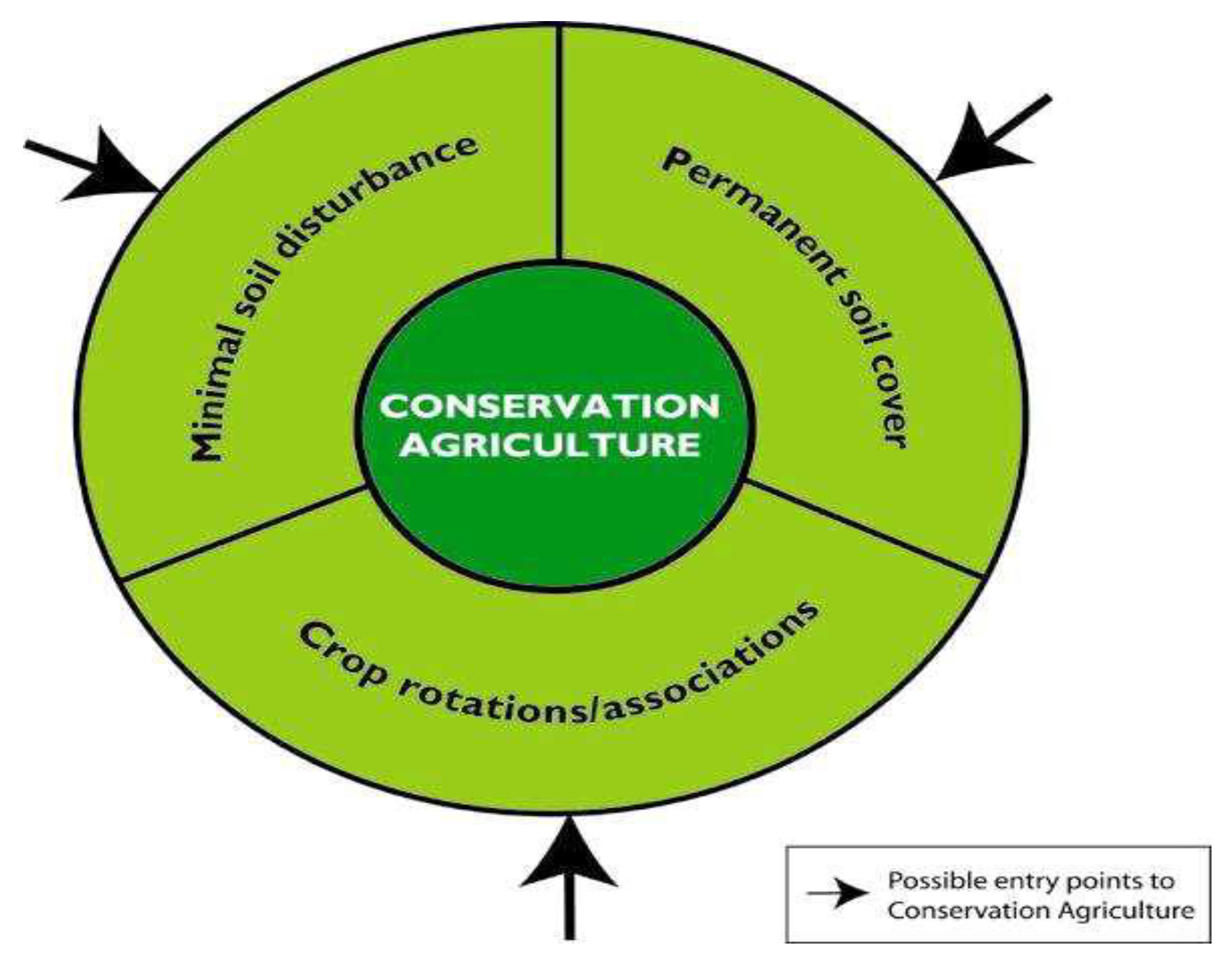
p < 0.01) significantly drive the count of CA practices adopted or rate ratio for CA adoption by smallholder farmers in the study area. Importantly, the basic CA practices adopted by farmers to preserve the ecosystem services in preferential order are: sequential rotation practice for different unrelated crops, the use of crop biomass for permanent soil cover, as well as minimum soil tillage. These findings partly agree with Abebe and Sewnet [62] who investigated determinants of soil conservation practices adoption in North-West Ethioia. Findings from their study indicated the influence of farmers’ and plot-level features, human capital, trainings and institutional support as the main drivers of adoption but never considered the role of social capital in adoption process which our study emphasized on. The importance of social capital in agricultural technologies adoption was also noted in the studies conducted by Hunecke et al. [10] and Husen et al. [9].
Similarly, the computed average marginal effects estimates in Table 3 revealed that, after controlling for other variables, on the average, farmers with appreciable years of farming experience used about 0.089 (8.9% points) of CA practices more than those with fewer years of experience in farming, and on average, farmers who were constantly in touch with extension officers adopted 0.896 (89.6% points) of CA practices more compared to those with less contact. Conversely, on the average, farmers who belong to many social groups adopted 1.304 points of CA practices less than those who belong to fewer social groups. The implication of this is that activities of social groups in the study area tend to tilt towards social engagement alone other than sharing useful and beneficial information about agricultural technologies. This result also reinforced the earlier submission made about the social groups in the study areas. Meanwhile, as indicated in Table A2, the evaluation of information measures (that is, Akaike’s and Bayesian Information Criterion—AIC and BIC) clearly revealed that negative binomial regression model fits better, owing to a smaller AIC and BIC statistics values. This is in line with Williams [54,63].

3.2.2. Goodness-of-Fit Test/Fit-Test Statistics

Evidently, it is clear from the result presented in Table A3 that both the negative binomial model and zero-inflated negative binomial model consistently fit better than either of the Poisson model or zero-inflated Poisson model. Importantly, BIC favors the negative binomial regression model while AIC favors the zero-inflated negative binomial model. This finding also provides the necessary and sufficient condition that the Poisson regression model is unfit for the estimation in question because it suffers from an over-dispersion problem. Hence, the justification for the use of the negative binomial model to examine the effects of social capital viz-a-viz social networks on CA adoption counts in South-Western Nigeria.

3.2.3. Marginal Treatment Effects Estimates: Empirical Results

The MTE model estimation was fitted through local IV and separate approach estimators with reference to parametric assumptions. However, the local IV was favored due to the model performance. The output from this estimation as shown in Table 4 highlights the impact evaluation of the specified covariates on the outcomes as measured by farmers’ farm income. Likewise, the differences in the average outcomes across the fitted covariates could be inferred directly from the first panel of the output as indicated by β0. In this instance, the coefficient for years of farming experience in the first panel of the output table indicates that one more year of farming experience translates into approximately 1.83% higher income, albeit with a non-linear effect. Arising from this, it is difficult to confidently infer that it is the actual effects of extra years of farming experience that drives the higher income if we fail to observe a strong exogeneity assumption as required on the fitted covariates. Equally, the coefficient of farm size under CA system from the first panel of the output table also suggests that an extra hectarage of farm size leads to about 25.22% decrease in farmers’ income. However, without accounting for strong exogeneity assumption on this factor, this reason alone cannot substantiate the farmers’ inability to produce within the production possibility frontier, given the economies of scale in terms of farm size increase.
In a similar manner, the second panel of the output with β1β0 in Table 4 explains the observed differences in treatment effects across covariate values, which also indicates treatment status and covariate interactions. Thus, the coefficient for gender indicates that a male farmer has 6.12 points higher advantage in terms of income generated as a result of CA adoption. The coefficient for age of the farmers suggests that an increase in age translates to about a 34.2% increase in farmers’ income, while an extra year of formal education suggests a farmer has about a 40.2% increase in income. However, the estimated coefficient for years of farming experience suggests than an increase in this farmers’ characteristics translates to approximately 10.86% decrease in the farmers’ income, while an extra increase in farm size under the CA system suggests about a 2.93-point increase in farmers’ income ceteris paribus. Similarly, an increase in the farmers’ total farm size indicates an approximately 1.02-point decrease in these farmers’ income which is somewhat erroneous and contrary to expectation; given the economies of scale in terms of farm size increase and all else equal, an increase in total farm size is expected to drive increased farm output and by extension, increased farmers’ income. The results also indicated that social capital is a significant factor towards CA adoption, but the benefits of social interaction is not maximally explored based on the direction of movement of this variable; that is, an increase in social capital benefits was found to drive an approximately 1.27-point decrease in farmers’ revenue. More so, the coefficients of extension delivery services (i.e., access and frequency of access) translated to about an 8.02-point decrease and a 5.34-point increase in farmers’ income, respectively, suggesting that the performance of an extension delivery system in the study area was not optimal. Importantly, for regional factor influence, a region (that is, Oyo State region) was arbitrarily set to be the basis of comparison since few research institutes (such as the International Institute of Tropical Agriculture (IITA)) are domiciled in this region. Therefore, compared to the counterpart farmers in region1 (Oyo State), the coefficients of region2 and region3 (Osun and Ondo states) suggest that an increase in adoption of CA by farmers in these regions will induce about a 4.29-point decrease and a 6.61-point increase in farmers’ income, respectively, all else equal. However, drawing conclusions on the treatment by relying on these findings alone without accounting for the possible non-linear effects may be erroneous and misleading for a valid, tenable, and causal inference about these findings.
To this effect, the third panel in the output table addressed this concern where under different treatment effects parameters and policy changes. The full distribution of marginal treatment effects parameters presented include: average treatment effects (ATEs), average treatment effects on the treated (ATT), average treatment effects on the untreated (ATUT—the spill-over effects), as well as the policy relevant treatment effects (MPRTEs—which points at the average effects of making marginal shifts to the propensity scores for both the treated and untreated individuals). This is also necessary to fully understand the treatment effects heterogeneity in relation to the framework guiding MTEs potential from a hypothetical policy that shifts the propensity to choose treatment which is the CA adoption. More importantly, as noted by Zhou and Xie [64], this approach preserves all of the treatment effects heterogeneity that is consequential for selection bias. In lieu of this, the output from the third panel highlighting the average difference in the outcome between the treated and untreated groups revealed that ATT > ATE > ATUT > LATE 0; such that, income is higher among the farmers who adopted the CA system than the counterparts who did not adopt CA for whom average income is virtually zero. More so, these treatment effects parameters are statistically significant at various levels; but an exception is made of ATT which is not significant at any level. However, MPRTEs estimated under the stylized policy changes represented by MPRTE1, MPRTE2, and MPRTE3 respectively indicate a substantial marginal income among these farmers (treated group). It is important to note that the exact magnitude of MPRTE depends heavily on the form of the policy change, especially under the normal parametric model which this study considered. For instance, under the first policy change where the policy changes increase everyone’s probability of adopting CA by the same amount, the parametric estimate of MPRTE is −8.527, suggesting that an extra effort to adopt CA would translate to about an 8.5-point decrease in farmers’ income among the marginal entrants on CA adoption. Equally, under the second policy change where this change favors farmers who appear more likely to adopt CA, the marginal income is approximately a 7.3-point decrease if there is a change in policy that permits and increases everyone’s probability of adopting CA proportionally. Besides, this scenario can even go as high as about a 12.5-point decrease in income under the third policy change where the change favors those farmers who appear less likely to adopt CA. However, the same pattern of results is observed under the polynomial MTEs model. The implication of this is that a different policy experiment could increase or decrease CA adoption, depending on which individuals it induces to gain and attract the expected spread and exposure.
In addition, considering the p-values for the two statistical tests shown in Table 4, the first one represents a joint test for the second panel of the output β1
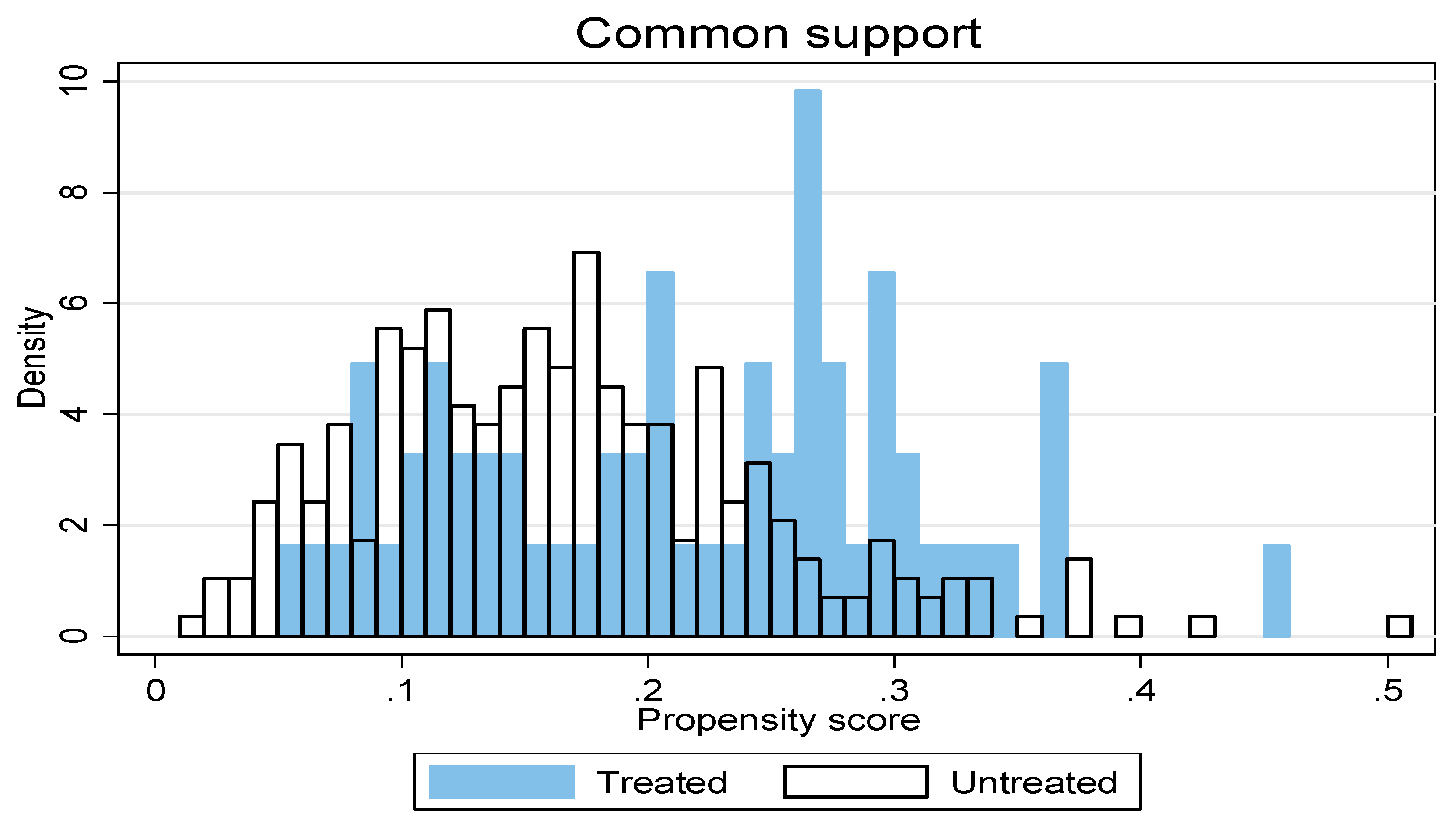
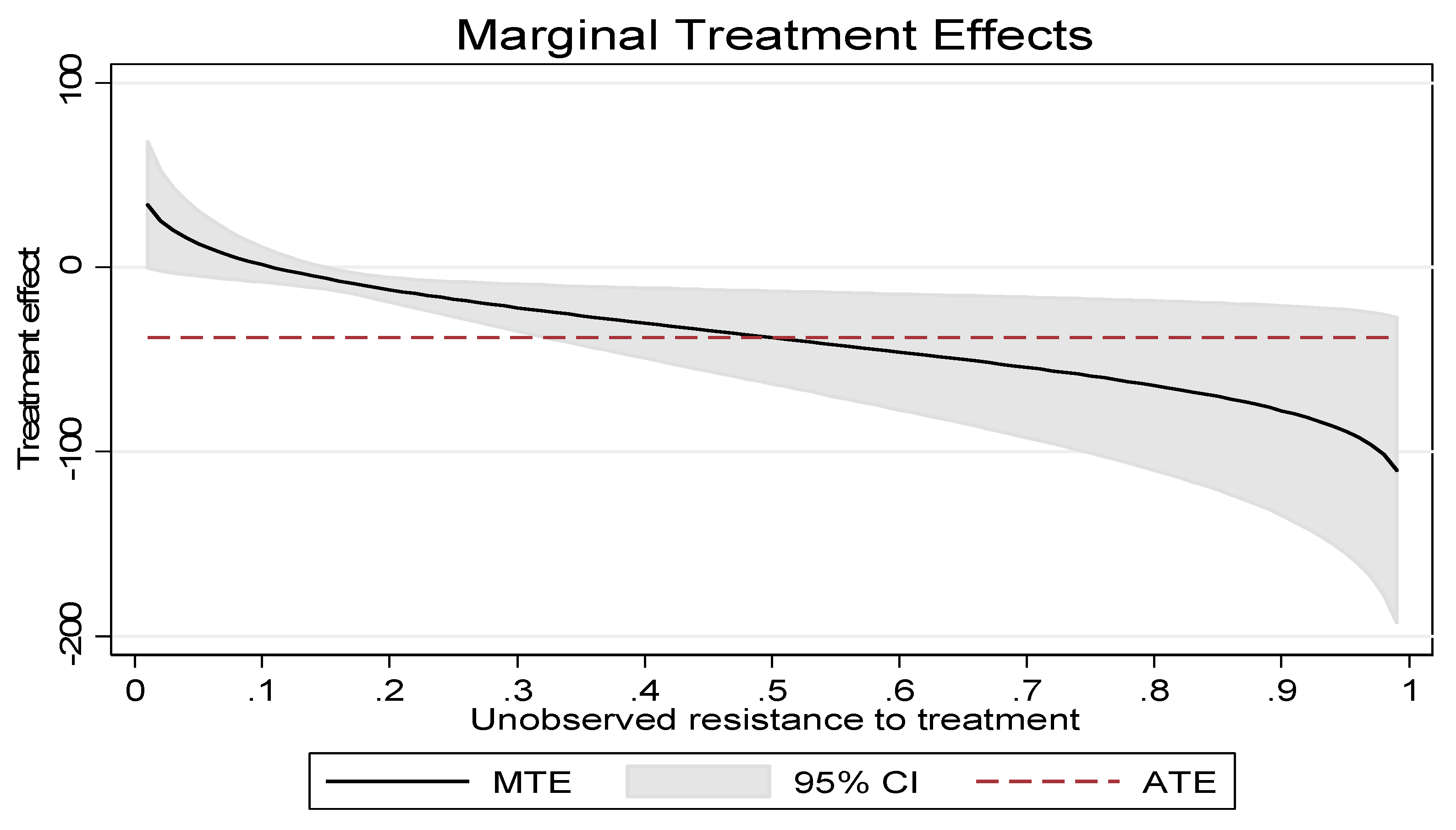
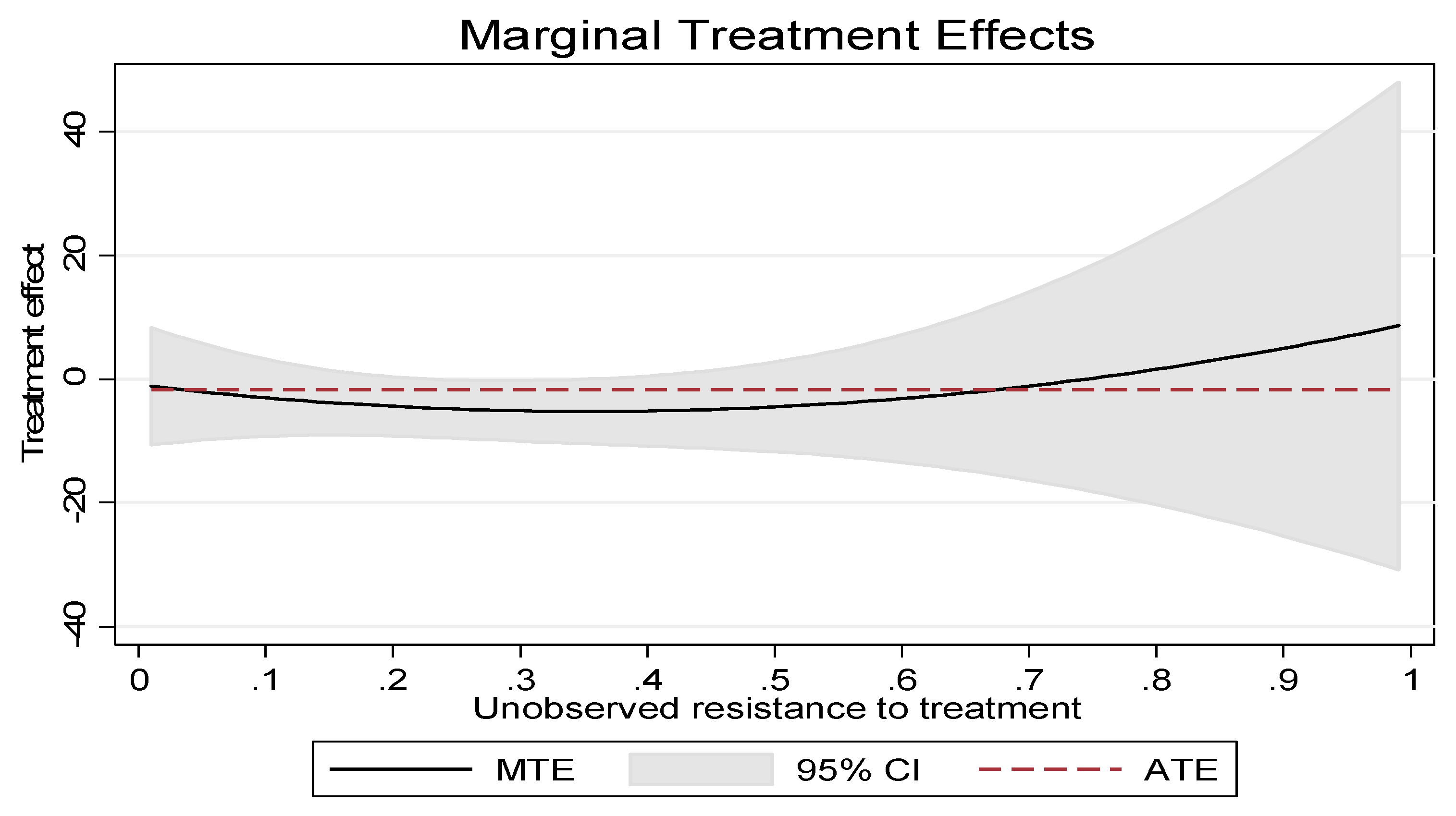
β0, which is also a test of whether the treatment effect differs across the covariates. The second one indicates a test for essential heterogeneity, which is also a joint test of all coefficients in k(u). From all indications, the first test revealed that the treatment effects differ significantly across the covariates in the second panel of output while the second test indicated that the treatment effects vary significantly with unobserved heterogeneity in the sample. Evidently, there are significant differences in the treatment effects across the sample. Therefore, this finding suggests that different policy scenarios or situations could increase or decrease CA adoption, depending on which individuals it induces to attract the expected spread and exposure. However, for parametric joint normal assumption using local IV, Figure 3 and Figure 4 depict the density distribution of propensity scores, MTE curve plot, as well as the associated confidence intervals for the treated and untreated farmers. This will permit to make necessary inferences about the common support. In this case, downward sloping of the estimated MTE plot is observed, with relatively high treatment effects at the beginning of the UD distribution (addressing propensity not to be treated), which eventually declines to negative effects at the right end of the distribution. This pattern of slope (downward) is in tandem with Roy model which predicts a positive selection on unobservable benefits.
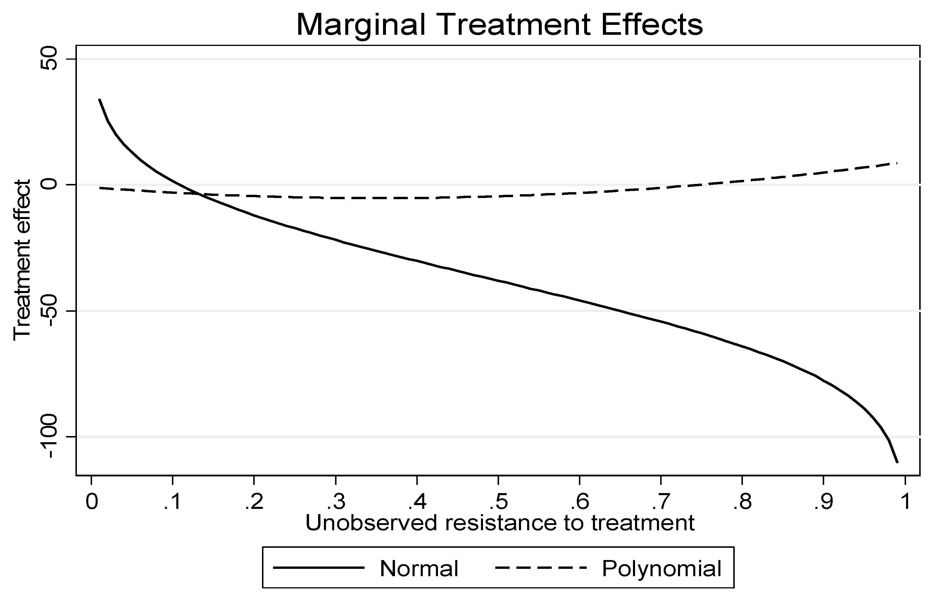
For robust estimation, this study further applied parametric polynomial MTE model and the separate estimation approach by relaxing the joint normal distribution assumption as well as plotting MTE curves for both normal and polynomial functions of the MTE models as indicated in Figure 5 and Figure 6, respectively. Here, the MTE plot for normal is downward sloping with negative treatment effects, which is consistent with the first estimate while MTE plot for the polynomial is relatively flat at the start of the UD distribution. This eventually slopes upward above zero towards the tail end of the 
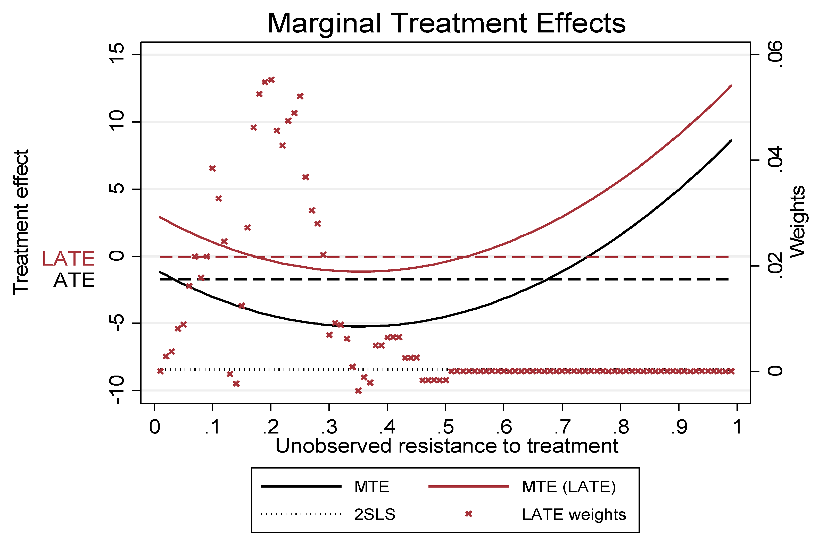
UD distribution. Similarly, treatment parameter weights were estimated and the resultant plots are shown in Figure 7. In this case, the MTE curve at the average of the covariate and the MTE curve for adopters are evidently convex upward; that is, the plots slope consistently upward without overlapping from the start to the end of 
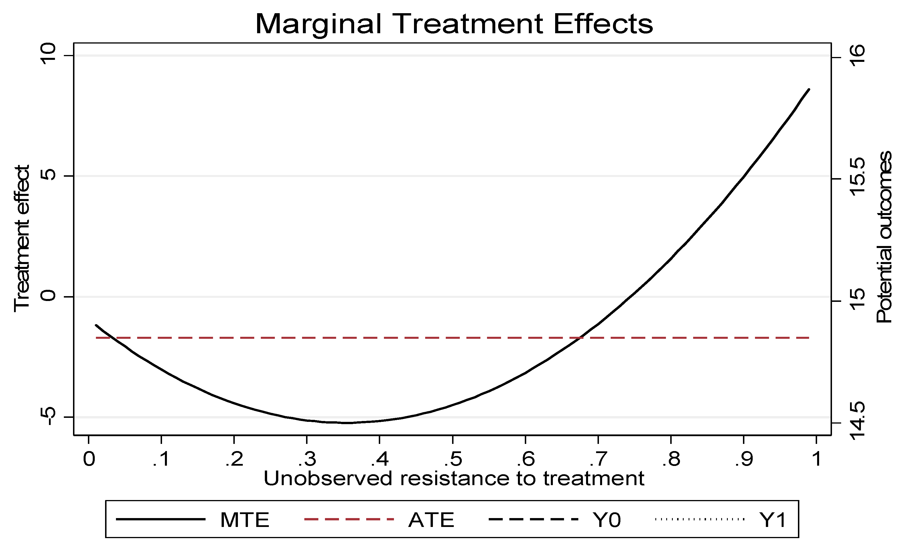
UD distribution. This suggests that farmers are motivated to adopt CA because of the instrumented participation in collective action (social capital) have different values of covariate. Therefore, this influences the treatment but not the outcome. However, the weight distribution indicated that the adopters have a much lower probability to have unobserved resistance towards the mid-point of the distribution. This further suggests that the farmers have MTEs slightly above the average. Hence, the farmers (adopters) who are influenced by the instrument are the ones with slightly above average increase in farm income. Similarly, separate estimation procedure was carried out in fitting the polynomial model by plotting the resulting potential outcomes to investigate if the observed MTE downward plot trend is generated by upward slopping of Y1, and downward sloping of Y0, or a combination of the two scenarios. Recall that the difference between outcome for the treated Y1 and outcome for the untreated Y0 represents MTE. Therefore, the plot as shown in Figure 8 indicated that though these farmers are relatively similar, the farmers who have high resistance to treatment perform poorly in terms of income realized from farm output than their low resistance counterparts who are also adopters. Hence, it can be inferred that, all else equal, there is a substantial effects and impacts of the treatment (that is, adoption of CA practices) on the farmers’ farm income.

4. Concluding Remarks and Policy Statements

Conclusively, the study found that farmers’ years of farming experience (p < 0.1), frequency of visits by the extension agents (p < 0.05), and social capital viz-a-viz density of social groups membership (p < 0.05) significantly determined the count of CA practices adopted with varying degrees by smallholder farmers in the study area. Although social capital expressed in terms of membership of occupational group and diversity of social group members also had positive influence on the count of CA practices adopted, but these features were not significant owing largely to the “information gaps” about the improved agricultural technologies. Suffice it to say that, there is the possibility of apathy among the farmers within the social structure to acquire more information about the improved agricultural technology because of the long-term benefits associated with adoption of CA alternative practices; hence, activities of various social groups, importantly, farmers’ occupational group largely center on social engagements.
Therefore, from the findings, the study highlighted the relevance of gender in lieu of the count of CA technologies adopted. Equally, the skewed pattern of CA adoption towards male gender as a significant predictor of adoption was also revealed. Therefore, there is a need to address the core issue of women marginalization in farming activities and farming related policies, most especially the bias towards women in land tenure arrangement. Importantly, there is need for a greater re-visitation of extension delivery systems associated with diffusion of information about CA practices in Nigeria through continuing and ongoing supports of extension services using farmer-led extension approaches facilitated by public extension agencies and NGOs saddled with outsourced extension services. On a general note, findings from count model mirror the significant importance and positive impact of social capital accumulation viz-a-viz social networks in the adoption process. The underlying aim is to understand peer group influence within a social structure impact diffusion of information among networks members and how to constantly explore these links to promote effective dissemination and flow of information on improved agricultural technologies towards sustained adoption of CA in Nigeria. Similarly, since policy relevant treatment effects indicated that different policy scenarios or situations could increase or decrease CA adoption, depending on which individuals it induces to attract the expected spread and exposure, there is a need to intensify the effort and policies to change the reality of farming especially among smallholder farmers in Africa and Nigeria in particular, from the traditional, inappropriate and unproductive tillage-based farming systems to a more and highly-productive, profitable, sustainable, and environmentally sound conservation agriculture system.

Author Contributions

S.O.O. conceptualized the study, conducted the research, and wrote the draft manuscript while A.M. reviewed, edited, and validated the manuscript. All authors therefore approved the final manuscript.

Funding

This research received no external funding.

Conflicts of Interest

The authors declare no conflict of interest.

Appendix A

Table A1. Quantiles of estimated probabilities (Goodness-of-fit test).
GroupProbObs_1Exp_1Obs_0Exp_0Total
10.067751.73033.335
20.089612.83432.235
30.115823.63331.435
40.133664.42930.635
50.160335.23229.835
60.182946.03129.035
70.208946.83128.235
80.2431127.92327.135
90.3086109.42525.635
100.52111413.22121.835
Number of observations = 350, number of groups = 10. Hosmer–Lemeshow chi2 (8) = 15.47, prob > chi2 = 0.0507. Source: Data analysis, 2018.
Table A2. Akaike’s information criterion and Bayesian information criterion.
ModelObs.ll(null)ll(model)dfAICBIC
Poisson350−1548.42−1462.76132951.533001.68
Negative Binomial350−966.08−948.65141925.301979.31
Source: Data analysis, 2018.
Table A3. Tests and Fit Statistics.
PRMBIC = 376.870AIC = 6.769PreferOverEvidence
vs. NBRMBIC = −171.005diff = 547.875NBRMPRMVery strong
AIC = 5.193diff = 1.576NBRMPRM
LRX2 = 553.733prob = 0.000NBRMPRMp = 0.000
vs. ZIPBIC = 121.142diff = 255.728ZIPPRMVery strong
AIC = 6.006diff = 0.764 ZIPPRM
Vuong = 5.241prob = 0.000ZIPPRMp = 0.000
vs. ZINBBIC = −160.147diff = 537.017ZINBPRMVery strong
AIC = 5.191diff = 1.578 ZINBPRM
NBRMBIC = −171.005AIC = 5.193PreferOverEvidence
vs. ZIPBIC = 121.142diff = −292.147NBRMZIPVery strong
AIC = 6.006diff = −0.813NBRMZIP
vs. ZINBBIC = −160.147diff = −10.858NBRMZINBVery strong
AIC = 5.191diff = 0.002 ZINBNBRM
Vuong = 1.323prob = 0.093ZINBNBRMp = 0.093
ZIPBIC = 121.142AIC = 6.006PreferOverEvidence
vs. ZINBBIC = −160.147diff = 281.289ZINBZIPVery strong
AIC = 5.191diff = 0.815ZINBZIP
LRX2 = 287.147prob = 0.000ZINBZIPp = 0.000
Source: Data analysis, 2018. Note that: PRM = Poisson regression model; NBRM = Negative binomial regression model; ZIP = Zero inflated poisson model; ZINB = Zero inflated negative binomial regression model.

References

  1. Oyakhilomen, O.; Zibah, R.G. Agricultural Production and Economic Growth in Nigeria: Implication for Rural Poverty Alleviation. Q. J. Int. Agric. 2014, 53, 207–223. [Google Scholar]
  2. Kassie, M.; Pender, J.; Yesuf, M.; Köhlin, G.; Bluffstone, R.; Mulugeta, E. Estimating returns to soil conservation adoption in the Northern Ethiopian Highlands. Agric. Econ. 2008, 38, 213–232. [Google Scholar] [CrossRef]
  3. IIRR; ACT. Conservation Agriculture. A manual for farmers and extension workers in Africa. In International Institute of Rural Reconstruction, Nairobi; African Conservation Tillage Network: Nairobi, Kenya, 2005. [Google Scholar]
  4. Silici, L. The Role of Social Capital in the Adoption and the Performance of Conservation Agriculture: The Practice of Likoti in Lesotho. Ph.D. Thesis, Departimento di Economia, Universita degli Studi Roma Tre, Rome, Italy, 2009. [Google Scholar]
  5. Kassam, A.; Friedrich, T.; Derpsch, R.; Lahmar, R.; Mrabet, R.; Basch, G.; González-Sánchez, E.J.; Serraj, R. Conservation Agriculture in the dry Mediterranean climate. Field Crops Res. 2012, 132, 7–17. [Google Scholar] [CrossRef]
  6. Ngwira, A.R.; Johnsen, F.H.; Aune, J.B.; Mekuria, M.; Thierfelder, C. Adoption and extent of conservation agriculture practices among smallholder farmers in Malawi. J. Soil Water Conserv. 2014, 69, 107–119. [Google Scholar] [CrossRef] [Green Version]
  7. Kassam, A.; Friedrich, T.; Derpsch, R.; Kienzle, J. Overview of the worldwide spread of Conservation Agriculture. Field Actions Sci. Rep. 2015, 8, 1–12. [Google Scholar]
  8. Pedzisa, T.; Rugube, L.; Winter-Nelson, A.; Baylis, K.; Mazvimavi, K. The Intensity of adoption of Conservation agriculture by smallholder farmers in Zimbabwe. Agrekon 2015, 54, 1–22. [Google Scholar] [CrossRef] [Green Version]
  9. Husen, N.A.; Loos, T.M.; Siddig, K.H. Social Capital and Agricultural technology Adoption among Ethiopian Farmers. Am. J. Rural Dev. 2017, 5, 65–72. [Google Scholar] [CrossRef]
  10. Hunecke, C.; Enger, A.; Jara-Rojas, R.; Poortvliet, P.M. Understand the Role of Social Capital in Adoption Decisions: An Application to Irrigation Technology. Agric. Syst. 2017, 153, 221–231. [Google Scholar] [CrossRef]
  11. D’Souza, A.; Mishra, A.K. Adoption and Abandonment of Partial Conservation Technologies in Developing Economies: The Case of South Asia. Land Use Policy 2018, 70, 212–223. [Google Scholar] [CrossRef]
  12. Silici, L.; Ndabe, P.; Friedrich, T.; Kassam, A. Harnessing sustainability, resilience and productivity through conservation agriculture: The case of likoti in Lesotho. Int. J. Agric. Sustain. 2011, 9, 1–8. [Google Scholar] [CrossRef]
  13. Calegari, A.; Ashburner, J. Further Experiences with Conservation Agriculture in Africa. In Proceedings of the 18th World Congress of Soil Science, Philadephia, PA, USA, 9–15 July 2006. [Google Scholar]
  14. Montemurro, F.; Fiore, A.; Campanelli, G.; Tittarelli, F.; Ledda, L.; Canali, S. Organic fertilization, green manure, and vetch mulch to improve organic zucchini yield and quality. HortScience 2013, 48, 1027–1033. [Google Scholar]
  15. EIP-AGRI Focus Group. Soil Organic Matter in Mediterranean Regions. 2015. Available online: http://www.ec.europa.eu/eip/agriculture/sites/agri-eip (accessed on 20 October 2018).
  16. Deligios, P.A.; Tiloca, M.T.; Sulas, L.; Buffa, M.; Caraffini, S.; Doro, L.; Sanna, G.; Spanu, E.; Spissu, E.; Urracci, G.R.; et al. Stable nutrient flows in sustainable cropping systems of globe artichoke. Agron. Sustain. Dev. 2017, 37, 1–12. [Google Scholar] [CrossRef]
  17. Ndah, H.T.; Schuler, J.; Uthes, S.; Zander, P. Adoption Decision Theories and Conceptual models of Innovations Systems. In Proceedings of the CA2 Africa Inception Workshop, Leibniz-Centre for Agricultural Landscape Research (ZALF), Nairobi, Kenya, 2–4 March 2010. [Google Scholar]
  18. Todaro, M.P.; Smith, S.C. Economic Development, 10th ed.; Pearson Addison Wesley: Boston, MA, USA, 2009. [Google Scholar]
  19. Hobbs, P.R. Conservation agriculture: What is it and why is it important for future sustainable food production. J. Agric. Sci. 2007, 145, 127–137. [Google Scholar] [CrossRef]
  20. De Lucas, A.I.; Molari, G.; Seddaiu, G.; Toscano, A.; Bombino, G.; Ledda, L.; Milani, M.; Vittuari, M. Multidisciplinary and Innovative Methodologies for Sustainable Management in Agricultural Systems. Environ. Eng. Manag. J. 2015, 14, 1571–1581. [Google Scholar]
  21. Deligios, P.A.; Chergia, P.A.; Sanna, G.; Solinas, S.; Todde, G.; Narvarte, L.; Ledda, L. Climate change adaptation and water saving by innovation irrigation management applied on open field globe artichoke. Sci. Total. Environ. 2019, 649, 461–472. [Google Scholar] [CrossRef] [PubMed]
  22. Foster, A.D.; Rosenzweig, M.R. Microeconomics of Technology Adoption. Annu. Rev. Econ. 2010, 2, 395–424. [Google Scholar] [CrossRef] [PubMed] [Green Version]
  23. Abdulai, A.; Owusu, V.; Bakang, J.E. Adoption of safer irrigation technologies and cropping patterns: Evidence from Southern Ghana. Ecol. Econ. 2011, 70, 1415–1423. [Google Scholar] [CrossRef] [Green Version]
  24. Awotide, B.A.; Diagne, A.; Awoyemi, T.T. Agricultural Technology Adoption, Market Participation and Rural Farming Households’ Welfare in Nigeria. In Proceedings of the 4th International Conference of the African Association of Agricultural Economists, Hammamet, Tunisia, 22–25 September 2013. [Google Scholar]
  25. Abdulai, A.; Huffman, W. The Adoption and Impact of Soil and Water Conservation Technology: An Endogenous Switching Regression Application. Land Econ. 2014, 90, 26–43. [Google Scholar] [CrossRef]
  26. Ademola, A.O.; Olujide, M.G. Soil Conservation Practices of Arable Crop Farmers in Atisbo Local Government Area of Oyo State, Nigeria. Adv. Res. 2014, 2, 878–888. [Google Scholar] [CrossRef]
  27. Afolami, C.A.; Obayelu, A.E.; Vaughan, I. Welfare impact of adoption of improved cassava varieties by rural households in South Western Nigeria. Agric. Food Econ. 2015, 3, 1–17. [Google Scholar] [CrossRef]
  28. Obisesan, A.A. Causal Effect of Off-Farm Activity and Technology Adoption on Food Security in Nigeria. AGRIS On-Line Pap. Econ. Inform. 2015, 7, 3–11. [Google Scholar]
  29. Wossen, T.; Bergen, T.; Di-Falco, S. Social capital, risk preference and adoption of improved farm land management practices in Ethiopia. Agric. Econ. 2015, 46, 81–97. [Google Scholar] [CrossRef]
  30. Pino, G.; Toma, P.; Rizzo, C.; Miglietta, P.; Peluso, A.; Guido, G. Determinants of farmers’ intention to adopt water saving measures: Evidence from Italy. Sustainability 2017, 9, 77. [Google Scholar] [CrossRef]
  31. Kirton, M. Adaptors and innovators: A description and measure. J. Appl. Psychol. 1976, 61, 622–629. [Google Scholar] [CrossRef]
  32. Rogers, E.M. What are innovators like? Theory Pract. 1963, 2, 252–256. [Google Scholar] [CrossRef]
  33. Oreszczyn, S.; Lane, A.; Carr, S. The role of networks of practice and webs of influencers on farmers’ engagement with and learning about agricultural innovations. Agric. Syst. 2010, 26, 404–417. [Google Scholar] [CrossRef]
  34. Lollo, E. Toward a theory of social capital definition: Its dimensions and resulting social capital types. In Proceedings of the 14th World Congress of Social Economics, Glasgow, UK, 20–22 June 2012. [Google Scholar]
  35. Hanifan, L.J. The Rural School Community Center. Ann. Am. Acad. Political Soc. Sci. 1916, 67, 130–138. [Google Scholar] [CrossRef]
  36. Nath, T.K.; Inoue, M.; Pretty, J. Formation and Function of Social Capital for Forest Resource Management and the Improved Livelihoods of Indigenous People in Bangladesh. J. Rural Community Dev. 2010, 5, 104–122. [Google Scholar]
  37. Putnam, R. Social capital: Measurement and consequences. Canad. J. Policy Res. 2001, 2, 41–51. [Google Scholar]
  38. Bowles, S.; Gintis, H. Social capital and community governance. Econ. J. 2002, 112, F419–F436. [Google Scholar] [CrossRef]
  39. Grootaert, C.; Bastelaer, T.V. Understanding and Measuring Social Capital: A Synthesis of Findings and Recommendations from the Social Capital Initiatives; Social Capital Initiative Working Paper No. 24; The World Bank: Washington, DC, USA, 2001. [Google Scholar]
  40. Woolcock, M. The place of social capital in understanding social and economic outcomes. Can. J. Policy Res. 2001, 2, 11–17. [Google Scholar]
  41. McCarthy, N.; Dutilly-Diane, C.; Drabo, B. Cooperation, collective action and natural resources management in Burkina Faso. Agric. Syst. 2004, 82, 233–255. [Google Scholar] [CrossRef]
  42. Jagger, P.; Luckert, M.K. Investments and returns from cooperative and household managed woodlots in Zimbabwe: Implications for rural afforestation policy. Land Use Policy 2008, 25, 139–152. [Google Scholar] [CrossRef]
  43. Aker, J.C. Social Networks and Household Welfare in Tanzania: Working Together to Get out of Poverty; University of California-Berkely: Berkeley, CA, USA, 2007. [Google Scholar]
  44. United Nations. Sustainable Development Knowledge Platform; Department of Economic and Social Affairs (UNDESA): New York, NY, USA, 2015; Available online: https://sustainabledevelopment.un.org/sdgs (accessed on 9 August 2018).
  45. Nguezet, P.M.D.; Diagne, A.; Okoruwa, V.O.; Ojehomon, V.E. Impact of Improved Rice Technology Adoption (NERICA varieties) on Income and Poverty among Rice Farming Households in Nigeria: A Local Average Treatment Effect (LATE) Approach. Q. J. Int. Agric. 2011, 50, 267–291. [Google Scholar]
  46. Oparinde, A.; Banerji, A.; Birol, E.; Ilona, P. Consumer Willingness to Pay for Biofortified Yellow Cassava: Evidence from Experimental Auctions in Nigeria; HarvestPlus Working Paper 13; International Food Policy Research Institute: Washington, DC, USA, 2014; pp. 1–2. [Google Scholar]
  47. Obisesan, A.A.; Amos, T.T.; Akinlade, R.J. Causal Effect of Credit and Technology Adoption on Farm Output and Income: The Case of Cassava Farmers in South-West Nigeria. In Proceedings of the 5th International Conference of the African Association of Agricultural Economists, Addis Ababa, Ethiopia, 23–26 September 2016. [Google Scholar]
  48. Awotide, B.A.; Karimov, A.A.; Diagne, A. Agricultural technology adoption, commercialization and smallholder rice farmers’ welfare in rural Nigeria. Agric. Food Econ. 2016, 4, 1–24. [Google Scholar] [CrossRef]
  49. National Space Research and Development Agency of Nigeria (NASRDA). Map of Nigeria Showing South-Western Region of Nigeria; NASRDA: Abuja, Nigeria, 2018.
  50. Corbeels, M.; Apina, T.; Koala, S.; Schuler, J.; Triomphe, B.; El Mourid, M.; Tittonell, P. Impact and Adoption of Conservation Agriculture in Africa: A Multi-Scale and Multi-Stakeholder Analysis; Centre de Coopération Internationale en Recherche Agronomique pour le Développement: Montpellier, France, 2010. [Google Scholar]
  51. Wooldridge, J.M. Econometric Analysis of Cross Section and Panel Data; MIT Press: Cambridge, MA, USA, 2010; pp. 265–268. [Google Scholar]
  52. Long, J.S.; Freese, J. Regression Models for Categorical Dependent Variables using STATA, 3rd ed.; Stata Press: College Station, TX, USA, 2014. [Google Scholar]
  53. Sebopetji, T.O.; Belete, A. An application of Probit analysis to factors affecting small-scale farmers’ decision to take credit: A case study of the Greater Letaba Local Municipality in South Africa. Afr. J. Agric. Res. 2009, 4, 718–723. [Google Scholar]
  54. Williams, R. Models for Count Outcomes. University of Notre Dame. 2015. Available online: https://www3.nd.edu/~rwilliam/ (accessed on 7 August 2017).
  55. Bruin, J. Newtest: Command to Compute New Test. UCLA: Statistical Consulting Group, 2006. Available online: https://stats.idre.ucla.edu/stata/ado/analysis/ (accessed on 2 April 2018).
  56. Andresen, M.E. Exploring marginal treatment effects: Estimation using STATA. Stata J. 2018, 18, 118–158. [Google Scholar] [CrossRef]
  57. Abadie, A.; Imbens, G.W. Matching on the estimated propensity score. Econometrica 2016, 84, 781–807. [Google Scholar] [CrossRef]
  58. Hosmer, D.W., Jr.; Lemeshow, S.A.; Sturdivant, R.X. Applied Logistic Regression, 3rd ed.; Wiley: Hoboken, NJ, USA, 2013. [Google Scholar]
  59. Baum, C.F. Models for Count Data and Categorical Response Data; Boston College and DIW Berlin, University of Adelaide: Adelaide, Australia, 2010; Available online: www.bc.edu/ec-c/s2013/327/S5CountCategorical0511.slides.pdf/ (accessed on 2 April 2018).
  60. Piza, E.L. Using Poisson and Negative Binomial Regression Models to Measure the Influence of Risk on Crime Incident Counts; Rutgers Center on Public Security: Newark, NJ, USA, 2012. [Google Scholar]
  61. Cameron, A.C.; Trivedi, P.K. Regression Analysis of Count Data, 2nd ed.; Cambridge University Press: New York, NY, USA, 2013. [Google Scholar]
  62. Abebe, Z.D.; Sewnet, M.A. Adoption of soil conservation practices in North Achefer District, Northwest Ethiopia. Chin. J. Popul. Resour. Environ. 2014, 12, 261–268. [Google Scholar] [CrossRef]
  63. Williams, R. Scalar Measures of Fit: Pseudo R2 and Information Measures (AIC and BIC); University of Notre Dame: Notre Dame, IN, USA, 2018; Available online: https://www3.nd.edu/~rwilliam/ (accessed on 7 August 2018).
  64. Zhou, X.; Xie, Y. Heterogeneous Treatment Effects in the Presence of Self-Selection: A Prospensity Score Perspective. 23 January 2018. Available online: https://scholar.harvard.edu/files/xzhou/ (accessed on 22 August 2018).
Figure 1. Basic principles of conservative agriculture (CA) practices. Source: Calegari and Ashburner [13] as cited in Ndah, Schuler, Uthes, and Zander [17].
Sustainability 11 00716 g001
Figure 2. Map of South-Western Nigeria showing the states and Local Government Areas (LGAs) of interest. Source: National Space Research and Development Agency of Nigeria (NASRDA) [49].
Sustainability 11 00716 g002
Figure 3. Common support for joint normal assumption. Source: Data analysis, 2018.
Sustainability 11 00716 g003
Figure 4. Marginal treatment effects plot for joint normal assumption. Source: Data analysis, 2018.
Sustainability 11 00716 g004
Figure 5. Marginal treatment effects plot for polynomial model (relaxing normal assumption). Source: Data analysis, 2018.
Sustainability 11 00716 g005
Figure 6. Marginal treatment effects plot for normal and polynomial models. Source: Data analysis, 2018.
Sustainability 11 00716 g006
Figure 7. Marginal treatment effects plot polynomial (using late memory). Source: Data analysis, 2018.
Sustainability 11 00716 g007
Figure 8. Marginal treatment effects plot (separate approach other than local IV). Source: Data analysis, 2018.
Sustainability 11 00716 g008
Table 1. Marginal effects (at the means) estimates of the binary probit model.
Delta-Method
Adoption of CAdy/dxstd. err.zp >|z|
1.gender0.06700.03951.70 ***0.089
Age0.00520.00271.92 ***0.054
years of formal education0.00850.00441.95 ***0.051
years of CA farming experience−0.00420.0024−1.73 ***0.083
farm size under CA cultivation0.01020.01800.570.570
log of output0.03410.02381.430.153
duration of residency0.00270.00221.210.225
labor contribution0.00050.00130.380.703
risk attitude0.11360.09551.190.235
1.access to extension service−0.23770.1680−1.410.157
frequency of extension visit0.08960.03572.51 *0.012
regional characteristics
  region 2−0.02370.0583−0.410.685
  region 30.01220.09690.130.900
Note: dy/dx for factor levels is the discrete change from the base level. * p < 0.01; *** p < 0.1 probability levels respectively. Source: Data analysis, 2018.
Table 2. Negative binomial regression model estimates.
Count of CA PracticesCoefficientIRRz-Statisticsp > |z|
1.gender−0.24210.7850−1.65 ***0.099
Age0.01211.01221.460.145
years of formal education0.00421.00420.280.777
1.land acquisition0.06391.06600.400.691
farm size cultivated under CA−0.01250.9876−0.200.841
total years of farming experience0.01341.01351.90 ***0.057
frequency of extension visits0.13451.14392.03 **0.042
1.occupational group membership0.14831.15980.920.357
1.participation in collective action−0.07530.9274−0.510.613
density-social groups membership−0.19560.8224−2.53 *0.011
diversity of social group members0.27971.32270.430.664
involvement in decision-making−0.71970.4869−1.180.239
constant−0.80220.4483−1.000.320
Ln (years of CA farming experience)11
Lnalpha0.21400.0914
Alpha1.23860.1132
Likelihood-ratio test of alpha = 0: chibar2 (01) = 1028.23, Prob >= chibar2 = 0.000. Number of observations = 350, Log likelihood = −948.64879, Dispersion = mean. Prob > chi2 = 0.0005, Pseudo R2 = 0.0180, LR chi2 (12) = 34.86. * p < 0.01; ** p < 0.05; *** p < 0.1 level respectively; IRR = incident rate ratio. Wald test of lnalpha: [lnalpha] _cons = 1; chi2 (1) = 73.91; prob > chi2 = 0.0000. Source: Data analysis, 2018.
Table 3. Average marginal effects estimates of the negative binomial model.
Count of CA Practicesdy/dxz-Statisticsp > |z|
1.gender −1.6770−1.560.118
Age0.08101.430.153
years of formal education0.02810.280.778
1.land acquisition0.41870.400.687
farm size cultivated under CA−0.0834−0.200.841
total years of farming experience0.08961.85 ***0.064
frequency of extension visit0.89662.00 **0.045
1.occupational group membership0.96050.940.347
1.participation in collective action−0.4935−0.510.608
density-social groups membership−1.3041−2.41 **0.016
diversity of social group members1.86500.430.664
involvement in decision-making−4.7995−1.170.243
* p < 0.01, ** p < 0.05, and *** p < 0.1, respectively. Note: dy/dx for factor levels is the discrete change from the base level. Source: Data analysis, 2018.
Table 4. Parametric marginal treatment effects estimates.
Log of Farmers’ Farm IncomeCoefficienttp > |t|
β0
1.gender−0.3044−0.920.359
Age−0.0176−0.780.437
years of formal education−0.0099−0.280.782
1.marital status0.02240.080.934
total years of farming experience0.01832.370.018 **
farm size cultivated under CA−0.2523−1.730.084 ***
total available farm size 0.08941.430.154
1.credit access0.01970.120.902
1.information acquisition−0.0125−0.070.942
index of social capital benefits0.08250.820.415
1.access to extension0.35040.650.518
frequency of extension visit−0.3312−0.340.218
regional factor
  20.39141.420.155
  3−0.1718−0.340.733
Constant11.7411.970.000 *
β1β0
1.gender6.123.080.002 *
Age0.342.530.012 *
years of formal education0.412.020.045 **
1.marital status2.191.380.167
total years of farming experience−0.11−2.630.009 *
farm size cultivated under CA2.933.460.001 *
total available farm size −1.02−2.730.007 *
1.credit access0.680.760.446
1.information acquisition1.401.500.134
index of social capital benefits−1.27−2.190.029 **
1.access to extension−8.02−2.370.019 **
frequency of extension visit5.343.140.002 *
regional factor
  2−4.29−2.760.006 *
  36.612.220.027 **
Constant−68.36−2.810.005 *
K
  Mills−30.91−2.430.016 **
Effects
parametric normal MTE model
(Local IV)
  Ate−38.03−2.970.003 *
  Att6.841.110.270
  Atut−47.52−2.870.004 *
  Late8.161.820.069 ***
  mprte1−8.53−3.050.003 *
  mprte2−7.28−2.500.013 *
  mprte3−12.48−3.570.000 *
parametric polynomial MTE model
(Separate approach)
  Ate−1.70−0.330.741
  Att−2.29−0.740.460
  Atut−1.58−0.250.799
  Late−0.09−0.040.967
  mprte1−3.74−1.610.107
  mprte2−3.87−1.550.122
  mprte3−4.30−1.850.065
Test of observable heterogeneity, p-value 0.0129 *
Test of essential heterogeneity, p-value 0.0157 *
* p < 0.01; ** p < 0.05; *** p < 0.1 level respectively. Note: mprtes indicate stylized marginal policy relevant treatment effects. Source: Data analysis, 2018.

