Developing Active Canopy Sensor-Based Precision Nitrogen Management Strategies for Maize in Northeast China

Abstract

Precision nitrogen (N) management (PNM) strategies are urgently needed for the sustainability of rain-fed maize (Zea mays L.) production in Northeast China. The objective of this study was to develop an active canopy sensor (ACS)-based PNM strategy for rain-fed maize through improving in-season prediction of yield potential (YP₀), response index to side-dress N based on harvested yield (RI_Harvest), and side-dress N agronomic efficiency (AE_NS). Field experiments involving six N rate treatments and three planting densities were conducted in three growing seasons (2015–2017) in two different soil types. A hand-held GreenSeeker sensor was used at V8-9 growth stage to collect normalized difference vegetation index (NDVI) and ratio vegetation index (RVI). The results indicated that NDVI or RVI combined with relative plant height (NDVI*RH or RVI*RH) were more strongly related to YP₀ (R² = 0.44–0.78) than only using NDVI or RVI (R² = 0.26–0.68). The improved N fertilizer optimization algorithm (INFOA) using in-season predicted AE_NS optimized N rates better than the N fertilizer optimization algorithm (NFOA) using average constant AE_NS. The INFOA-based PNM strategies could increase marginal returns by 212 $ ha⁻¹ and 70 $ ha⁻¹, reduce N surplus by 65% and 62%, and improve N use efficiency (NUE) by 4%–40% and 11%–65% compared with farmer’s typical N management in the black and aeolian sandy soils, respectively. It is concluded that the ACS-based PNM strategies have the potential to significantly improve profitability and sustainability of maize production in Northeast China. More studies are needed to further improve N management strategies using more advanced sensing technologies and incorporating weather and soil information.

1. Introduction

To achieve high grain yield and meet globally increasing food demand, over-application of nitrogen (N) fertilizer has been common in Chinese crop production [1,2,3]. Currently, maize (Zea mays L.) is the crop with the greatest demand for N fertilizer among all crops [4]. In China, the N recovery efficiency (RE) for maize is less than 30% [5]. Nitrogen fertilizer beyond the amount required by maize can escape from agricultural soils as reactive N (Nr), which can result in unintended adverse environmental and human health impacts [5,6]. Some of these environmental consequences, such as climate change and tropospheric ozone pollution, can also negatively affect crop yields [7,8]. N fertilizer related greenhouse gas (GHG) emissions (nitrous oxide under wet conditions and ammonia under hot conditions) have exceeded the corresponding gains in soil carbon related to its effect on increased biomass by 700% in China [9]. Therefore, optimizing N management for maize production to minimize the adverse environmental impacts is crucially important for sustainable development of agriculture [5,10].

The optimum N rate depends on crop N demand and soil N supply. The crop N demand is determined by the plant growth status and grain yield potential, while the soil N supply is a net result of mineralization, immobilization and losses of soil N. They are both influenced by many factors such as seasonal temperature, precipitation, physical and biogeochemical soil properties, and management history [11]. The interactions between soil water and N determine the growth, development and yield of maize. Efficient utilization of water and N can only be realized if they are closely matched [12]. Climate conditions can affect optimum N via various processes in soil such as nitrification, denitrification, leaching, and mineralization, which will modulate soil N availability to the crops [3,13,14,15,16]. Because of the temporal and spatial variability in climatic conditions and soil properties, the optimum N rate can vary widely across fields, within fields and over years in the same field [16,17,18]. The low N use efficiency (NUE) in China has been attributed to the poor synchrony between N fertilizer application and crop demand in space and time [17]. Therefore, precision N management (PNM) is needed to match N supply with crop N demand, both spatially and temporally, thereby improving NUE.

Crop growth responds to weather conditions, soil properties, and crop management. Crop growth status can reflect crop N demand and soil N supply [19,20]. N application rates are often adjusted for crop N requirements based on estimates of grain yield [21]. Active canopy sensors (ACSs) are commonly used to monitor crop growth status and make in-season N recommendations [22,23,24]. The GreenSeeker ACS (Trimble Navigation Limited, Sunnyvale, CA, USA) has been used to successfully predict maize grain yield potential during the growing season to improve in-season N side-dress recommendations [24,25,26]. Based on the N fertilization optimization algorithm (NFOA) developed by Raun et al. [27] using in-season estimation of yield potential and N response index (RI) estimated with GreenSeeker sensor, maize NUE was increased to 65% from 56% with a fixed rate split N application [28]. This algorithm has been adapted to PNM strategies for rice (Oryza sativa L.) in Northeast China, thereby increasing the N partial factor productivity (PFP) by 48% compared with farmer practices (FP), without significantly affecting rice grain yield [29]. The algorithm has also been adapted to PNM strategies for winter wheat (Triticum aestivum L.) and summer maize rotation in the North China Plain [30]. This PNM strategy significantly reduced N fertilizer applications and total apparent N losses while increasing NUE compared with both FP and regional optimum N management (RONM) [30].

In the NFOA algorithm, the first key component is the development of a model to estimate grain yield without additional N application (YP₀) based on mid-season canopy spectral measurements before side-dressing N application [31]. The second key component is to predict the grain yield response to additional N application, which is called response index (RI_Harvest) based on the ratio of harvested grain yield under sufficient N application over YP₀. For the GreenSeeker sensor, the normalized difference vegetation index (NDVI) is closely related to crop biomass and leaf area index and has been commonly used to predict YP₀ and RI_Harvest. The NDVI can become saturated at medium to high biomass conditions, so improvements are needed, especially under high yielding conditions [29,32,33,34]. One approach is to use ratio vegetation index (RVI) calculated using the reflectance of near infrared (NIR) over red waveband instead of NDVI, because RVI is less susceptible to the saturation effect of NDVI [29,34]. Another approach is to combine NDVI with plant height data to improve the estimation of plant biomass or maize yield [35,36]. Crop plant height as a single factor can be used to estimate the vegetative growth and potential yield of maize [37]. It is a highly sensitive growth parameter and is influenced by soil water content [38], texture [39], fertilizer rate [40], and cultivation methods [41]. A study by Machado et al. [42] indicated that plant height data could be used to explain 90% and 61% of the spatial and temporal variations in total dry matter and grain yield, respectively. More studies are needed to determine how much improvement can be made for in-season prediction of maize YP₀ and RI_Harvest, as well as side-dress or topdress N recommendation using RVI or plant height data.

After YP₀ and RI_Harvest are predicted, the grain yield with sufficient N application (YP_N) can be estimated by multiplying YP₀ and RI_Harvest. Then, the yield response to top-dress or side-dress N can be calculated, which is the difference between YP_N and YP₀. The N requirement can be calculated by multiplying this yield difference by grain N concentration. An N recovery efficiency (RE) value is needed to further estimate the amount of N fertilizer to be applied to meet the N requirement [27].

The N fertilizer need can also be calculated using yield response to N application divided by side-dress or top-dress N agronomic efficiency (AE_NS or AE_NT). Previously, constant NUE values were used in such algorithms. However, NUE is influenced by many factors, including N rate and timing, soil fertility status, residual N content, and environmental factors that can influence N losses through volatilization, soil denitrification, surface runoff, and leaching [43,44]. To improve the algorithm with more suitable NUE and grain N concentration values, Macnack et al. [45] found that preplant N, GreenSeeker NDVI, rainfall, and growing degree days (GDD) combined and explained 76% of winter wheat grain protein content variability, but NDVI, rainfall, and average temperature combined could not predict NUE. In another study of winter wheat, 37% and 45% of NUE variabilities were explained using RI_Harvest or RI_Harvest plus RI_NDVI [46]. More studies are needed to determine how maize NUE can be estimated in-season and how can such updated NUE can improve active sensor-based in-season N recommendations for maize.

Northeast China is the most important and the largest rain-fed maize production region of the country, accounting for 35% of China’s maize production (China’s National Bureau of Statistics, 2015). To improve the N management of spring maize in this region, the GreenSeeker sensor has been used for in-season diagnosis of maize N status, with an accuracy of 81% and 71% at V7-V8 and V9-V10 growth stages, respectively [34]. However, no ACS-based PNM strategies have been developed for Northeast China yet. Therefore, the specific objectives of this study were to: (1) Evaluate the potential of improving in-season prediction of YP₀ and RI_Harvest by adding plant height information; (2) predict side-dress N agronomic efficiency (AE_NS) prior to the side-dress N application, and (3) develop an ACS-based PNM strategy for rain-fed maize in Northeast China.

2. Materials and methods

2.1. Study Site Description

This study site is located in Lishu County (43°02′–43°46′N, 123°45′–124°53′E), Jilin Province in Northeast China. Approximately 70% of the total cropland is planted with maize in this county. Two fields with contrasting soil types, black soil (loamy clay) equivalent to typic Haploboroll and aeolian sandy soil (loamy sand) equivalent to typic Cryopsamments according to the United States Department of Agriculture (USDA) Soil Taxonomy, were selected for this study. Soil characteristics are summarized in

Table 1. Basic soil properties for the experimental fields.

Soil Type	Soil Texture	Bulk Density (g cm−3)	Field Capacity (cm cm−3)	pH	Total N (g kg−1)	Soil OM (g kg−1)	Available-P (mg kg−1)	Exchangeable K (mg kg−1)
Black soil	Silt loam	1.40	0.39	5.5	1.35	26.2	35.4	129
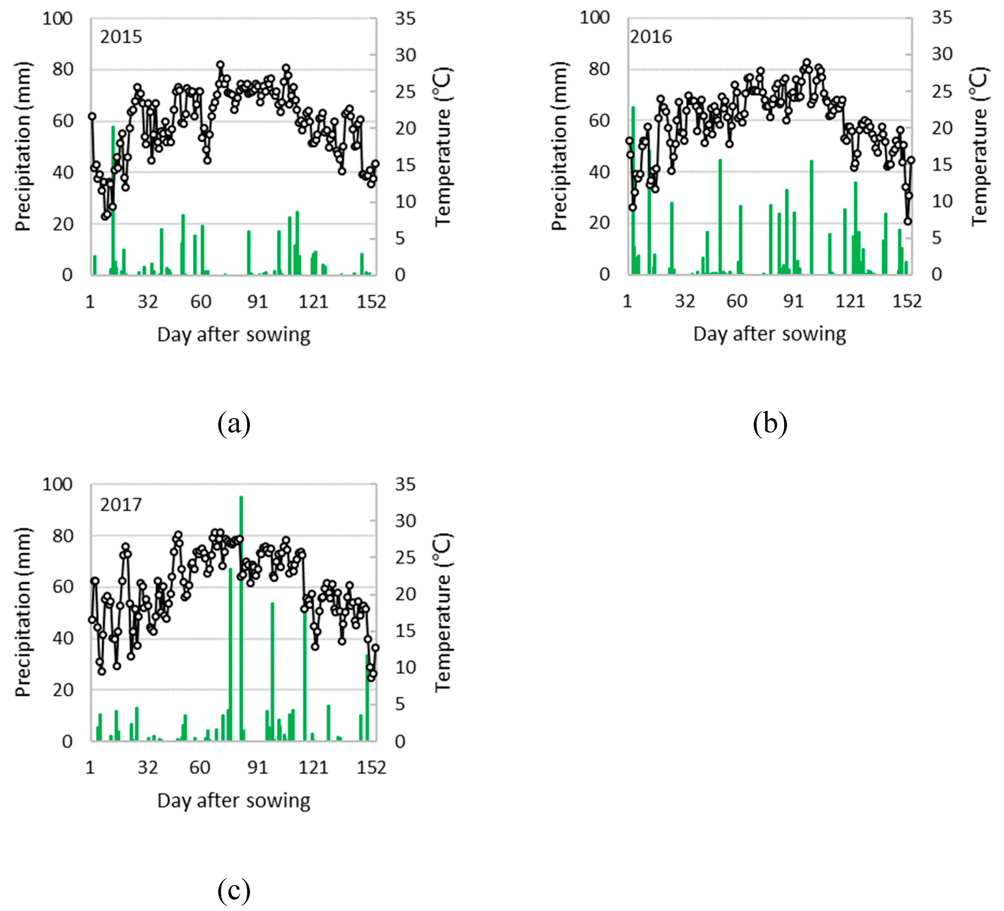
Aeolian Sandy soil	Loamy sand	1.65	0.13	6.0	0.65	9.7	30.8	73

. This study site is located in the North Temperate Zone, which is characterized by a semi-humid continental monsoon climate. The mean annual average temperature is 6.6 °C, the annual sunshine is 2656 h, the average annual frost-free period is 142 days, and the annual cumulative temperature (>10 °C) is 3,056 °C. The annual average precipitation is 556 mm, about 84% of which occurs during the crop growing season from May to September. The precipitation distribution and GDD during the study years (2015-2017) in Lishu County are shown in Figure 1. According to precipitation accumulated during the whole growth period, 2015, 2016, and 2017 were considered dry, wet, and normal years, respectively.

2.2. Experimental Design

The same experimental treatments were implemented in both black and aeolian sandy soil fields from 2015 to 2017. A split-plot design with three replications was applied for the experiment, with three planting densities (D1: 55,000, D2: 70,000, D3: 85,000 plant ha⁻¹) as the main plots and seven N fertilizer rates (N0: 0, N1: 60, N2: 120, N3: 180, N4: 240, N5: 300, and N6: 60 kg N ha⁻¹) being the subplots. The N5 treatment was not included in the first year of this experiment in 2015, but later found to be necessary and added in 2016 and 2017. Therefore, the N4 (240 kg ha⁻¹) treatment was used as the sufficient-N fertilizer subplot in 2015, while the N5 (300 kg ha⁻¹) treatment was used in 2016 and 2017. The N fertilizer for N1–N5 was applied in two splits: 1/3 was broadcasted and embedded into soil as basal N using ammonium sulfate and 2/3 was band applied as side-dress N using urea at the V8–V9 stage. Each subplot with an area of 108 m² (9 m width × 12 m length, with 1 m wide alley between the subplots) was divided into two parts: 2/3 of the subplot (part 1) received the rest of the N application at V8–V9 as planned, while 1/3 of the subplot (part 2) did not receive side-dress N application at the V8–V9 stage. Part 2 subplots were used to develop ACS-based N recommendation algorithms. For N6, all N fertilizer was applied as basal fertilizer, and data from this treatment were used for evaluating N recommendation algorithms and PNM strategies. For each plot, sufficient phosphate (90 kg P₂O₅ ha⁻¹) and potash (90 kg K₂O ha⁻¹) fertilizer were applied before planting to make sure P and K nutrients were not limiting. The same local maize variety (Liangyu 66) was used in both fields. No irrigation was applied during the plant growth period for black soil field, while one-time irrigation of about 50 mm of water was applied before the anthesis growth stage in the aeolian sandy soil field each year. All plots were kept free of weeds, insects, and diseases with chemicals based on standard practices. These experiments were conducted in the same fields in all the three years.

2.3. Active Canopy Sensor Data Collection and Plant Sampling

The GreenSeeker ACS Model 505 was used in this study. This sensor detects crop canopy reflection in red (R: 650–670 nm) and near-infrared (NIR: 755–785 nm) spectral regions, allowing calculation of the NDVI and RVI [47]. At V8–V9 stage, the GreenSeeker sensor readings were collected by holding the sensor at approximately 0.7 m over the maize canopy in each subplot (four rows in the middle of subplots, and three meters length for each row) and walking at a constant speed. The sensor data from different rows in a subplot were averaged to represent that subplot. The NDVI and RVI values were calculated directly by the built-in software of the GreenSeeker sensor. After sensing, three representative plants were selected and plant height was measured manually from the stem bottom to the leaf top by extending the uppermost leaf as high as possible in each subplot. At the maturity stage, grain yield was determined by manually harvesting eight lows with three meters in length except the border rows in each subplot and standardized to 14% grain moisture content. The stem, leaf, and grain were separated and oven-dried at 105 °C for 30 min, then dried at 70 °C to a constant weight, and finally weighed to obtain the plant aboveground biomass (AGB), later they were ground into fine powder to determine plant nitrogen concentration (PNC) by a modified Kjeldahl digestion method [48].

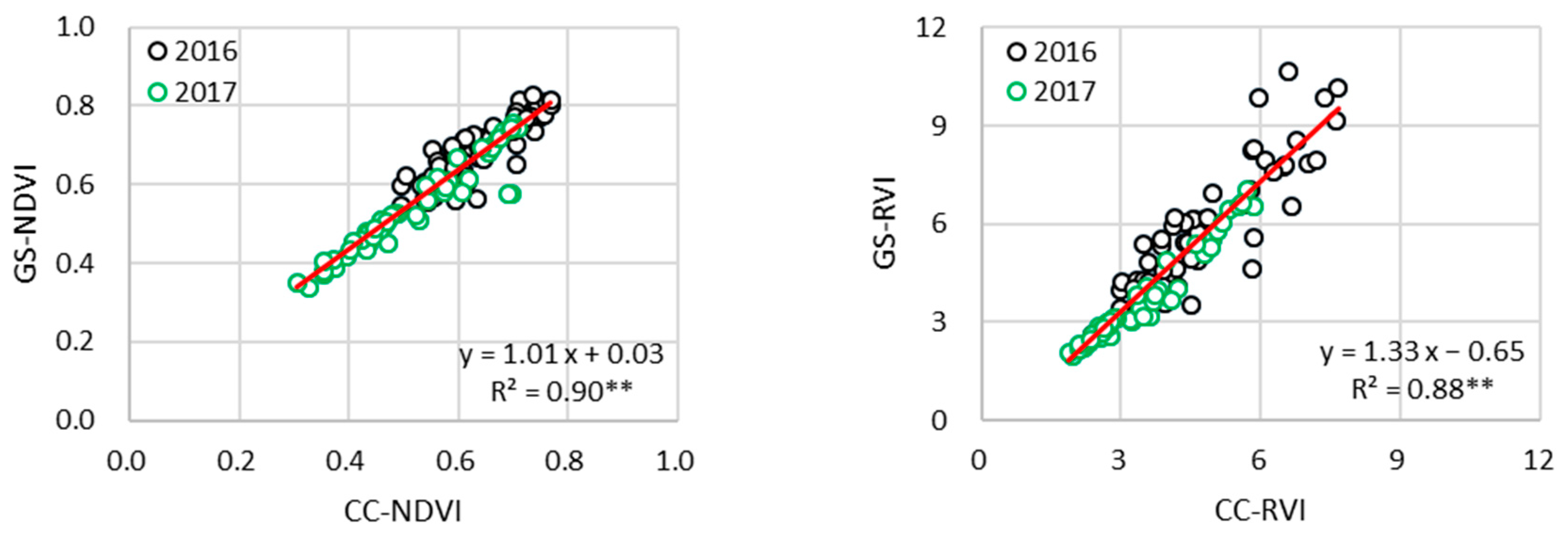
The GreenSeeker sensor data were missing from the aeolian sandy soil field in 2015, but a Crop Circle ACS 430 sensor (Holland Scientific, Inc., Lincoln, NE, USA) was used to collect reflectance data in all the study fields and yields. The measurement method for the Crop Circle ACS 430 sensor was similar with the GreenSeeker in the sensing position, time, height, and speed. Strong relationships were found between the NDVI and RVI values from Crop Circle ACS 430 and GreenSeeker (Figure 2), and as a result, the GreenSeeker NDVI and RVI values in the sandy field in 2015 were converted from NDVI and RVI values of Crop Circle ACS 430 sensor.

2.4. The Development of N Fertilizer Recommendation Algorithm

Plant height can vary among varieties with the same N conditions, as well as from year to year due to seasonal conditions within the same variety. Therefore, we normalized plant height measurement in this study and used the relative height (RH) together with vegetation. It was calculated as follows:

RH = H from a TSP/Average H from SNSP

(1)

where H was plant height, TSP was test subplot, SNSP was sufficient-N fertilizer subplot (SNSP).

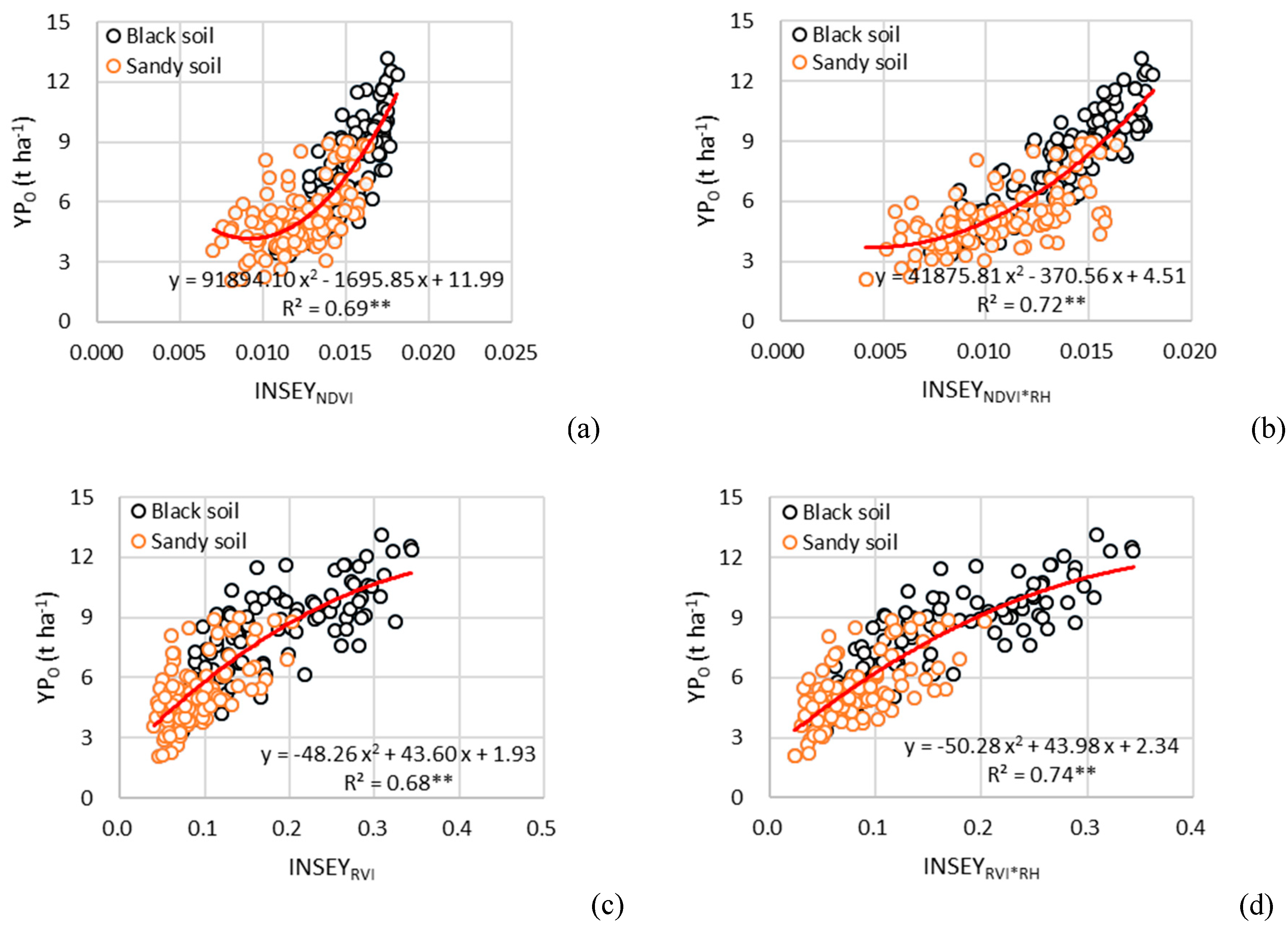
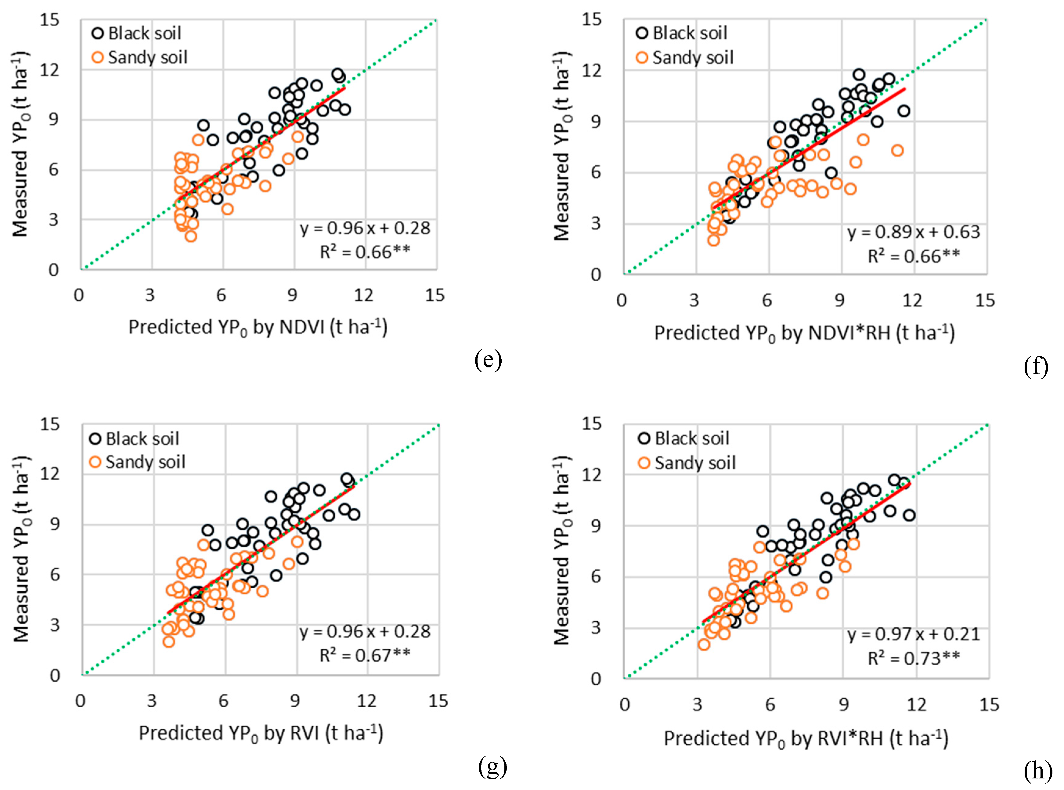
Grain yield potential without side-dress N fertilizer (YP₀) was estimated using the in-season estimate of yield (INSEY) based on NDVI (RVI) or NDVI (RVI) with RH (INSEY_NDVI, INSEY_RVI, or INSEY_NDVI*RH, and INSEY_RVI*RH). They were calculated as follows:

INSEY_{NDVI (RVI, NDVI*RH, or RVI*RH)} = NDVI (RVI, NDVI*RH, or RVI*RH)/GDD

(2)

YP₀ = f (INSEY_{NDVI (RVI, NDVI*RH, or RVI*RH)})

(3)

where the GDD was the number of growing degree days greater than zero from planting to sensing.

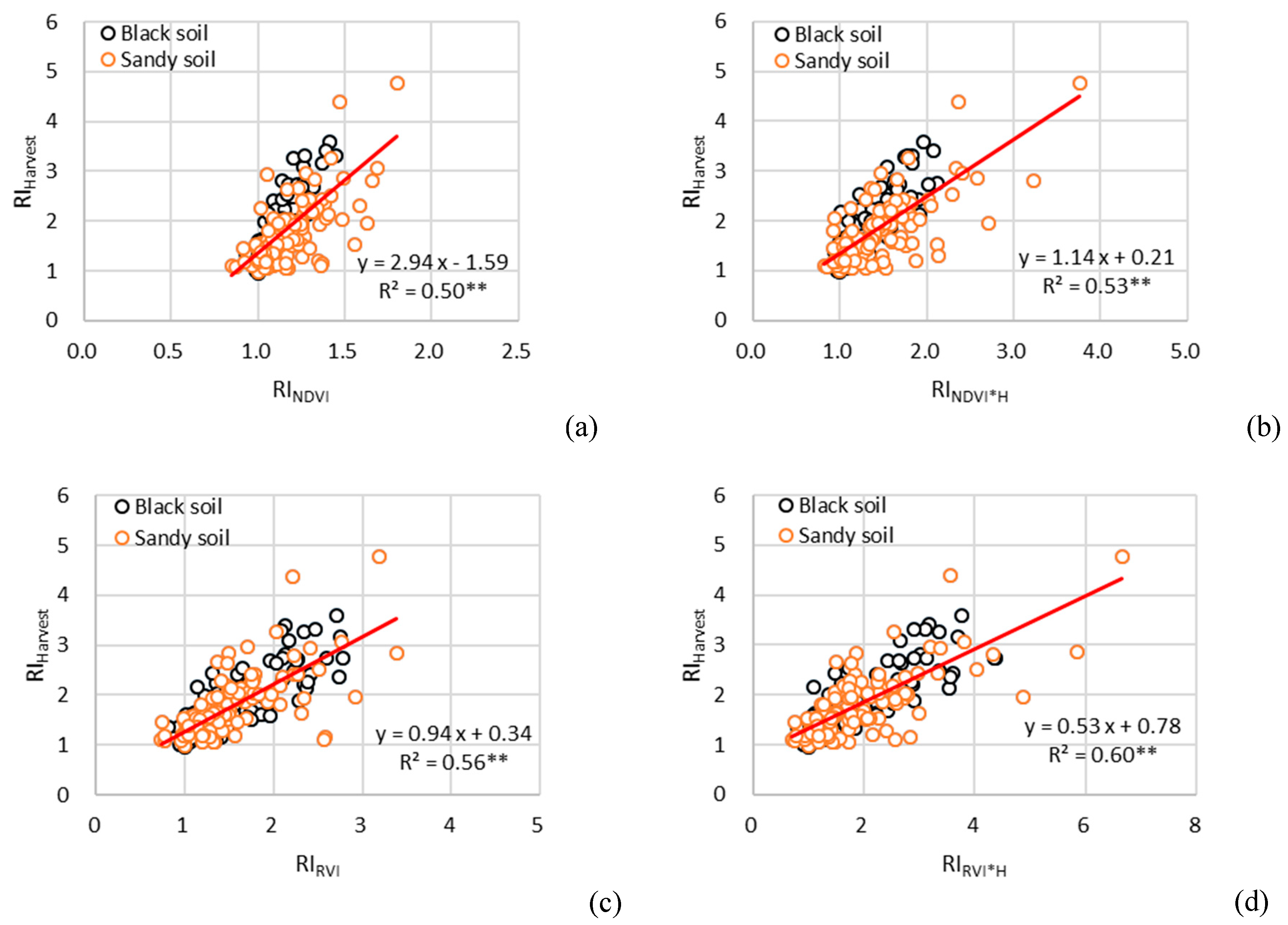
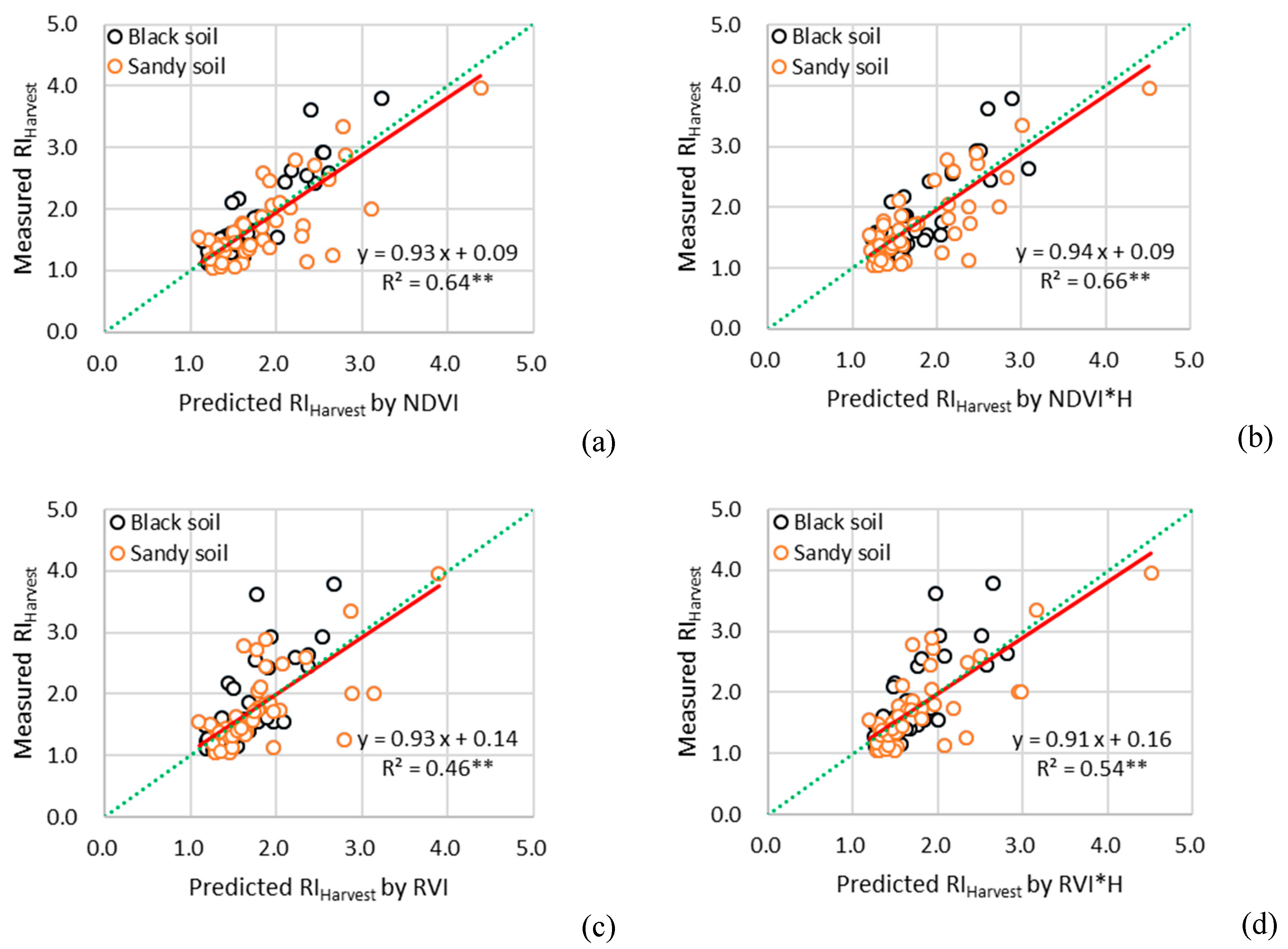
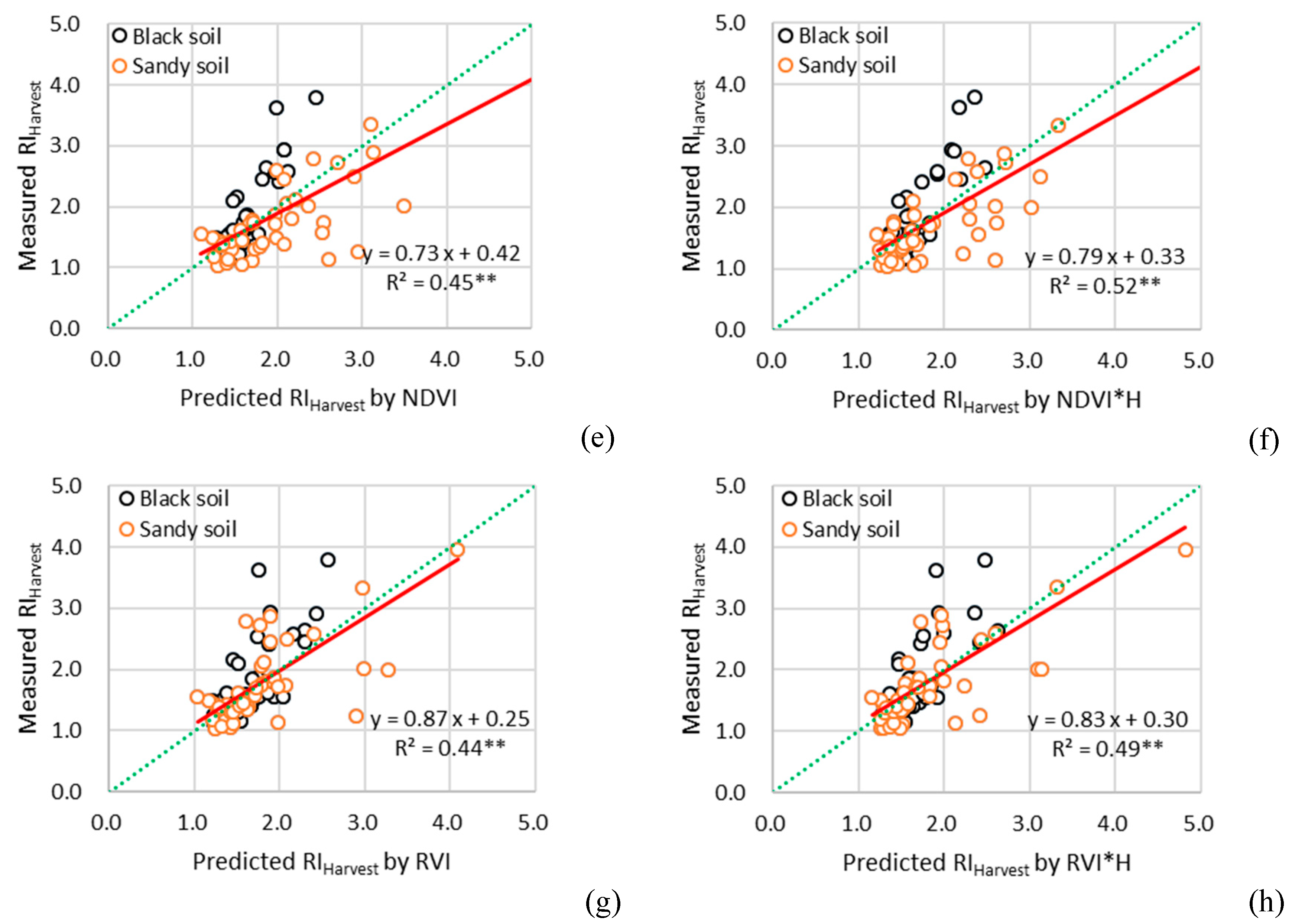
The grain yield response index to side-dress N fertilizer (RI_Harvest) was calculated using the average grain yield in the subplots receiving sufficient N fertilizer divided by the grain yield from a test subplot. RI_Harvest values were also estimated using the RI_NDVI and RI_RVI or RI_NDVI*H and RI_RVI*H at V8-V9 stage, which were calculated using average vegetation index in the subplots receiving sufficient N fertilizer divided by the average vegetation indices in a test subplot receiving different N rates. They were calculated as follows:

RI_Harvest = Average grain yield from SNSP/Grain yield from a TSP

(4)

RI_Height = Average plant height from SNSP/Plant height from a TSP

(5)

RI_{NDVI (RVI)} = Average NDVI (RVI) from SNSP/NDVI (RVI) from a TSP

(6)

RI_{NDVI*H (RVI*H)} = RI_Height × RI_{NDVI (RVI)}

(7)

RI_Harvest = f (RI_{NDVI (RVI, NDVI*RH, or RVI*RH)})

(8)

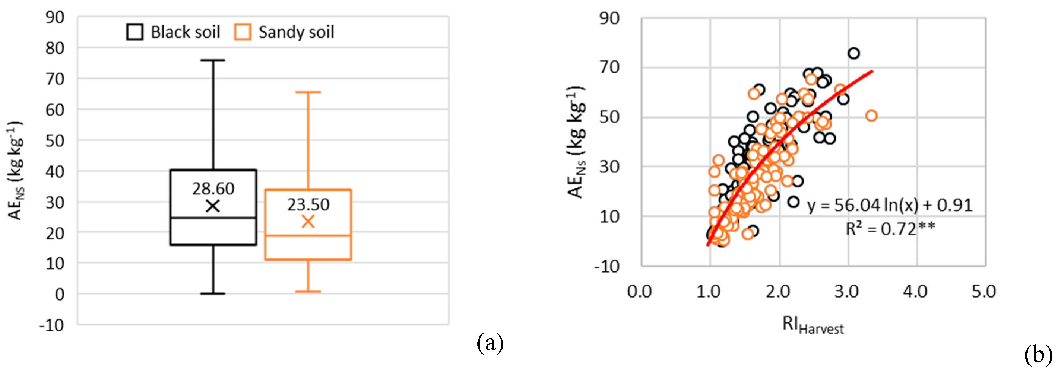
AE_NS was defined as the increased grain yield due to side-dress N application divided by the side-dress N fertilizer rate. In this study, AE_NS was calculated by dividing the increased grain yield (the grain yield from subplot part 1 minus the grain yield from subplot part 2) by the side-dress N fertilizer rate. It was calculated as follows:

AE_NS = (Yield from subplot part 1 − yield from subplot part 2)/N_SD

(9)

where N_SD was the side-dress N rate, kg ha⁻¹.

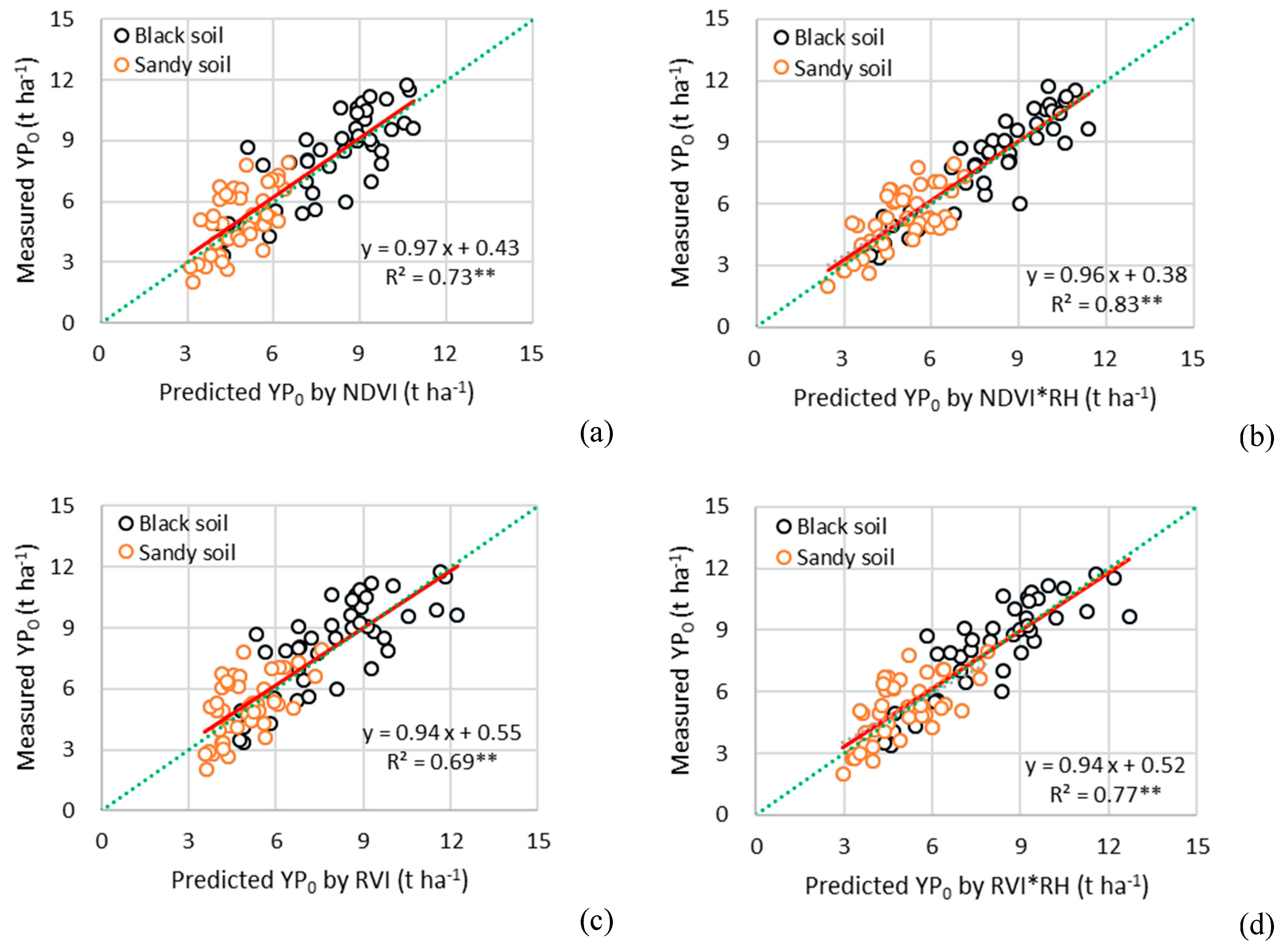
The YP₀, INSEY, RI_Harvest, and RI based on vegetation index data were randomly divided into two datasets: 70% of the data were used to establish models for estimating YP₀ and RI_Harvest, and 30% of the data were used for validation. The YP_N was calculated by multiplying the predicted YP₀ and the predicted RI_Harvest. Then the recommended N rate (Nrec) was calculated by dividing the difference between YP_N and YP₀ by the average AE_NS. In this study, an improved NFOA (INFOA) was developed by using in-season predicted AE_NS based on the in-season predicted RI_Harvest. They were calculated as follows:

AE_NS = f (RI_Harvest)

(10)

YP_N = YP₀ × RI_Harvest

(11)

Nrec = (YP_N − YP₀)/AE_NS

(12)

2.5. The Evaluation of N Recommendation Algorithms and Precision N Management Strategies

After the in-season YP₀, RI_Harvest and AE_NS prediction models were established and validated, sensor data from the subplot N6 (only receiving 60 kg N ha⁻¹ as basal N rate) at three planting densities were used to calculate the N recommendation rates using different N fertilizer recommendation algorithms at the V8–V9 stage. The economic optimum N rates (EONR), defined as the optimum N application rate resulting in the highest marginal return, were used to evaluate different N recommendation algorithms based on the GreenSeeker sensor.

The sensor-based PNM strategies were evaluated in terms of grain yield, marginal return, and NUE in comparison with the farmer practice (FP) and regional optimum management (ROM). For the black soil field, we defined the treatment with planting density of 70,000 plant ha⁻¹ and base N rate of 60 kg N ha⁻¹ (N6) as PNM treatment, and the treatment with planting density of 55,000 plant ha⁻¹ and total N rate of 300 kg N ha⁻¹ as FP treatment and the treatment with planting density of 70,000 plant ha⁻¹ and total N rate of 240 kg N ha⁻¹ as ROM treatment. For the aeolian sandy soil field, we defined the treatment with planting density of 55,000 plant ha⁻¹ and base N rate of 60 kg N ha⁻¹ as the PNM treatment. The FP and ROM treatments were the same as in the black soil field.

In this study, the grain yield and plant N uptake (PNU) from the different N recommendation algorithms and PNM strategies were calculated from the N response models of grain yield and PNU developed using data from treatments N0–N5.

The NUE indicators, partial factor productivity (PFP), agronomic efficiency (AE), and recovery efficiency (RE) were calculated using the following equations:

PFP (kg kg⁻¹) = Y_N/N_F

(13)

AE (kg kg⁻¹) = (Y_N − Y₀)/N_F

(14)

RE (%) =100 × (PNU_N − PNU₀)/N_F

(15)

where Y_N and Y₀ were the grain yield in N fertilizer application subplots and 0 kg N ha⁻¹ subplots, respectively, and PNU_N and PNU₀ were the PNU in N application subplots and 0 kg N ha⁻¹ subplots, respectively, and N_F was the applied N fertilizer rate.

The N surplus (N_S) was defined as N fertilizer application rate (N_F) minus PNU, which was calculated by multiplying plant N concentration by biomass.

The economic income, defined as marginal return to N (E, $ ha⁻¹), was calculated according to formula (16):

E = Y × P_Y − N_F × P_N

(16)

where Y was the grain yield (kg ha⁻¹), P_Y was the grain price ($ kg⁻¹), N_F was the N fertilizer application rate (kg ha⁻¹), P_N was the N fertilizer price ($ kg⁻¹). The prices of maize grain and N fertilizer were 0.31 and 0.62 $ kg⁻¹ in China, respectively [46].

2.6. Statistical Analysis

The standard deviation (SD), mean, and coefficient of variation (CV, %) of maize yield indicators were calculated using Microsoft Excel (Microsoft Corporation, Redmond, WA, USA). The coefficient of determination (R²) relating vegetation indices with yield indicators was calculated using SPSS 19 (SPSS Inc., Chicago, Illinois, USA). The overall performance of the established relationships was estimated by comparing R² and root mean square error (RMSE) of prediction. The higher the R² and the lower the RMSE, the higher the precision and accuracy of the prediction models. The N response models of grain yield and plant N uptake to N rate were determined by SAS Version 8.0 (SAS Institute Inc., Cary, NC, USA). The least significant difference (LSD) test at 5% and 1% probability levels were used for the analysis of difference.

3. Results

3.1. Variation of Grain Yield and Plant Height

Maize grain yield and plant height were significantly affected by the factors of soil type, year, and N, but not by plant density (

Table 2. Significance of mean squares in the analysis of variance under three plant densities (D) and six N rates (N) combined across three years (Y) for two soil types (S).

Source of Variation	df	Significance of Mean Square
		YP0 (t ha−1)	Height (cm)
Soil (S)	1	***	***
Year (Y)	2	***	***
Density (D)	2	ns	ns
Nitrogen (N)	5	***	***
S × Y	2	***	***
S × D	2	ns	ns
S × N	5	***	ns
Y × D	4	**	ns
Y × N	9	***	***
D × N	10	*	ns
S × Y × D	4	*	ns
S × Y × N	9	ns	ns
S × D × N	10	ns	ns
Y × D × N	18	ns	ns
S × Y × D × N	18	ns	ns
Error	204	0.85	62.60

Note: *, **, and *** indicate significance at 0.05, 0.01, and 0.001 probability levels, respectively. ns = non-significant.

). They varied greatly across different fields, years, and treatments (

Table 3. Descriptive statistics for maize grain yield potential (YP₀), N response index based on harvested yield (RI_Harvest), relative plant height (RH), and N response index based on plant height (RI_Height) across soils, years, and N treatments.

Soil Type	n	YP0 (t ha−1)				RIHarvest				RH				RIHeight
		Range	Mean	SD	CV (%)	Range	Mean	SD	CV (%)	Range	Mean	SD	CV (%)	Range	Mean	SD	CV (%)
Calibration data
Black soil	109	3.34–13.15	8.02	2.37	30	0.96–3.59	1.77	0.63	36	0.60–1.05	0.89	0.11	12	0.95–1.68	1.14	0.16	14
Aeolian sandy soil	109	2.08–8.94	5.18	1.55	30	0.99–4.77	1.76	0.66	37	0.48–1.19	0.86	0.14	16	0.84–2.08	1.20	0.23	19
Across soils	218	2.08–13.15	6.60	2.45	37	0.96–4.77	1.76	0.64	36	0.48–1.19	0.87	0.13	14	0.84–2.08	1.17	0.20	17
Validation data
Black soil	44	3.36–11.74	8.09	2.31	29	1.08–3.80	1.74	0.66	38	0.59–1.05	0.90	0.11	12	0.95–1.68	1.13	0.16	14
Aeolian sandy soil	44	2.01–7.95	5.12	1.49	29	1.04–3.96	1.74	0.65	37	0.52–1.15	0.87	0.16	19	0.87–1.91	1.20	0.25	21
Across soils	88	2.01–11.74	6.60	2.44	37	1.04–3.96	1.74	0.65	38	0.52–1.15	0.88	0.14	16	0.87–1.91	1.17	0.21	18

). For calibration data, the grain yield and RI_Harvest were more variable across fields (CV = 36–37%) than the relative plant height and RI based on plant height (RI_Height) (CV = 14–17%). The black soil field had similar variation (CV = 30–36%) as the aeolian sandy soil field (CV = 30–37%) in grain yield and RI_Harvest, respectively. For the relative plant height and RI_Height, the aeolian sandy soil field had slightly higher variability (CV = 16–19%) than the black soil field (CV = 12–14%). The validation dataset had similar trends as the calibration dataset.

3.2. In-season Prediction of Yield Potential (YP₀)

The relationships between YP₀ and GreenSeeker NDVI or RVI with or without relative plant height information (INSEY) are shown in

Table 4. The soil-specific and general models and coefficients of determination (R²) for the relationships between vegetation indices (NDVI, NDVI*RH, RVI, and RVI*RH) and grain yield potential (YP₀) as well as response index (RI_Harvest) in different soils across three years.

Variable (y)	Index (x)	Black Soil		Aeolian Sandy Soil		Across Soils
		Equation	R2	Equation	R2	Equation	R2
YP0	INSEYNDVI	y = 54740.93 × x 2.12	0.68 **	y = 187.15 × x 0.82	0.26 **	y = 91894.1 × x2 − 1695.85 × x + 11.99	0.69 **
	INSEYRVI	y = 21.79 × x 0.57	0.64 **	y = 15.21 × x 0.45	0.30 **	y = −48.26 × x2 + 43.6 × x + 1.93	0.68 **
	INSEYNDVI*RH	y = 2175.68 × x 1.31	0.78 **	y = 105.65 × x 0.67	0.45 **	y = 41875.81 × x2 − 370.56 × x + 4.51	0.72 **
	INSEYRVI*RH	y = 21.60 × x 0.53	0.74 **	y = 15.35 × x 0.43	0.44 **	y = −50.28 × x2 + 43.98 × x + 2.34	0.74 **
RIHarvest	RINDVI	y = 5.24 × x − 3.99	0.78 **	y = 2.47 × x − 1.16	0.46 **	y = 2.94 × x − 1.59	0.50 **
	RIRVI	y = 1.04 × x + 0.21	0.69 **	y = 0.86 × x + 0.46	0.46 **	y = 0.94 × x + 0.34	0.56 **
	RINDVI*H	y = 1.85 × x − 0.58	0.72 **	y = 0.97 × x + 0.35	0.52 **	y = 1.14 × x + 0.21	0.53 **
	RIRVI*H	y = 0.61 × x + 0.68	0.69 **	y = 0.48 × x + 0.85	0.54 **	y = 0.53 × x + 0.78	0.60 **

Note: ** indicates the significance in the level of 0.01.

and Figure 3. INSEY_NDVI*RH and INSEY_RVI*RH could explain more variability in YP₀ (44–78%) than INSEY_NDVI and INSEY_RVI (26–68%) in both fields. The relationships between YP₀ and INSEY were stronger in the black soil field (R² = 0.64–0.78) than in the aeolian sandy soil field (R² = 0.26–0.45). Across fields, INSEY_NDVI*RH and INSEY_RVI*RH performed similarly as INSEY_NDVI and INSEY_RVI for estimating YP₀ (R² = 0.68–74%).

The validation results of in-season prediction of YP₀ are shown in

Table 5. Validation results for soil-specific and general models using vegetation indices to predict grain yield potential (YP₀) and response index (RI_Harvest) across three years.

Model	Variable (y)	Index (x)	Black Soil			Aeolian Sandy Soil			Across Soils
			R2	RMSE	RE	R2	RMSE	RE	R2	RMSE	RE
Soil-specific model	YP0	INSEYNDVI	0.66 **	1.34	0.17	0.36 **	1.18	0.23	0.73 **	1.26	0.19
		INSEYRVI	0.60 **	1.44	0.18	0.32 **	1.22	0.24	0.69 **	1.34	0.20
		INSEYNDVI*RH	0.82 **	0.97	0.12	0.51 **	1.03	0.20	0.83 **	1.01	0.15
		INSEYRVI*RH	0.73 **	1.19	0.15	0.43 **	1.11	0.22	0.77 **	1.16	0.18
	RIHarvest	RINDVI	0.82 **	0.28	0.16	0.57 **	0.42	0.24	0.64 **	0.39	0.22
		RIRVI	0.57 **	0.43	0.25	0.45 **	0.48	0.27	0.46 **	0.48	0.27
		RINDVI*H	0.73 **	0.34	0.20	0.65 **	0.38	0.22	0.66 **	0.38	0.22
		RIRVI*H	0.60 **	0.41	0.24	0.56 **	0.42	0.24	0.54 **	0.44	0.25
General model across soils	YP0	INSEYNDVI	0.64 **	1.37	0.17	0.25 **	1.28	0.25	0.66 **	1.41	0.21
		INSEYRVI	0.62 **	1.40	0.17	0.31 **	1.23	0.24	0.67 **	1.39	0.21
		INSEYNDVI*RH	0.79 **	1.04	0.13	0.37 **	1.17	0.23	0.66 **	1.42	0.21
		INSEYRVI*RH	0.75 **	1.14	0.14	0.40 **	1.14	0.22	0.73 **	1.26	0.19
	RIHarvest	RINDVI	0.82 **	0.28	0.16	0.57 **	0.42	0.24	0.45 **	0.48	0.28
		RIRVI	0.57 **	0.43	0.25	0.45 **	0.48	0.27	0.44 **	0.49	0.28
		RINDVI*H	0.73 **	0.35	0.20	0.65 **	0.38	0.22	0.52 **	0.45	0.26
		RIRVI*H	0.60 **	0.41	0.24	0.57 **	0.42	0.24	0.49 **	0.46	0.27

Note: ** indicates significance at the level of P ≤ 0.01, RMSE is the root mean square error, RE is the relative error.

. The general models across soil types (R² = 0.62–0.79) performed similarly as the soil-specific models (R² = 0.60–0.82) in the black soil field, but the soil-specific models (R² = 0.32–0.83) performed better than the general models (R² = 0.25–0.73) in the aeolian sandy soil or across soils. INSEY_NDVI*RH and INSEY_RVI*RH (R² = 0.37–0.83) performed consistently better in predicting YP₀ than INSEY_NDVI and INSEY_RVI (R² = 0.25–0.73) (Table 5, Figure 4).

3.3. In-season Prediction of Maize Yield Responsiveness to N Side-dressing (RI_Harvest)

The relationships between RI_Harvest and RI based on GreenSeeker NDVI or RVI with or without plant height information are shown in Table 4 and Figure 5. Across soils, RI_NDVI*H and RI_RVI*H explained slightly more variability in RI_Harvest (53−60%) than RI_NDVI and RI_RVI (50−56%). In the aeolian sandy soil field, RI_NDVI*H and RI_RVI*H explained more variability in RI_Harvest (52−54%) than RI_NDVI and RI_RVI (46%), while there was no improvement in the black soil field. The relationships between RI_Harvest and RI based on sensor data were stronger in the black soil field (R² = 0.69−0.78) than aeolian sandy soil field (R² = 0.46−0.54).

The validation results for in-season prediction of RI_Harvest are shown in Table 5 and Figure 6. The general models performed the same as the soil-specific models in the black and aeolian sandy soil fields, and the soil-specific models performed better across soils. The addition of plant height information improved model performance in the aeolian sandy soil field (R²=0.56−0.65 vs. 0.45−0.57).

3.4. The Relationship between AE_NS and RI_Harvest

AE_NS values varied significantly across N rates, planting densities and site-years (Figure 7). The average AE_NS value was 28.6 and 23.5 kg kg⁻¹ in the black and aeolian sandy soils, respectively. AE_NS had a strong relationship with RI_Harvest (R² = 0.72−0.74) (

Table 6. The average AE_NS (kg kg⁻¹) and its relationship with RI_Harvest.

Soil	AENS (kg kg−1)	Equation	R2
Black soil	28.60	AENS = 57.52×ln (RIHarvest) + 2.68	0.74 **
Aeolian sandy soil	23.50	AENS = 54.37×ln (RIHarvest) − 0.77	0.72 **
Across soils	26.05	AENS = 56.04×ln (RIHarvest) + 0.91	0.72 **

Note: ** indicates significance at the level of P ≤ 0.01.

). Therefore, the AE_NS can be predicted using the in-season predicted RI_Harvest to improve the side-dress N fertilizer rate rather than using an average value.

3.5. Evaluating Different in-season N Recommendation Algorithms

Across fields, more INFOA recommendations (35–52%) fell within 10% of EONR than NFOA (4%–17%). This was true in either the black or aeolian sandy soil field (

Table 7. The percentage (%) of the recommended N rates falling within 10% of the economic optimum N rate (EONR) across three years. NDVI: Normalized difference vegetation index; RVI: Ratio vegetation index; NDVI-H: NDVI plus plant height information; and RVI-H: RVI plus plant height information.

Model	Soil	Algorithm	Percentage (%)
			NDVI	NDVI-H	RVI	RVI-H
Soil-specific model	Black soil	NFOA	7	19	7	7
		INFOA	33	44	41	63
	Aeolian sandy soil	NFOA	7	7	22	7
		INFOA	37	41	41	41
	Across soils	NFOA	7	13	15	7
		INFOA	35	43	41	52
General model	Black soil	NFOA	4	7	7	7
		INFOA	59	56	59	59
	Aeolian sandy soil	NFOA	19	26	0	11
		INFOA	26	33	30	37
	Across soils	NFOA	11	17	4	9
		INFOA	43	44	44	48

). In general, the addition of plant height information improved N recommendations, but the improvement was not consistent.

3.6. Evaluation of Sensor-based Precision N Management Strategies

The NFOA-based PNM strategies all resulted in higher PFP than INFOA-based PNM strategies, but the N surplus values were all negative, especially in the black soil (

Table 8. Comparison of the N rate (kg ha⁻¹), grain yield (t ha⁻¹), marginal return (MR) ($ ha⁻¹), N surplus (kg ha⁻¹), partial factor productivity (PFP) (kg ha⁻¹), agronomy efficiency (AE) (kg kg⁻¹), and recovery efficiency (RE) (%) for different N management strategies across three years in the black soil.

Management	Model	Algorithm	Index	N rate	Grain Yield	MR	N Surplus	PFP	AE	RE
CK				0	6.00	1860	−71.16
FP				300	12.21	3599	41.46	40.69	20.69	0.62
ROM				240	12.82	3827	11.42	53.44	28.43	0.66
PNM	Soil-specific model	NFOA	NDVI	163	11.77	3547	−31.17	72.33	34.84	0.75
			NDVI-H	190	12.21	3667	−16.55	64.46	33.18	0.72
			RVI	189	12.22	3672	−18.61	65.08	32.65	0.72
			RVI-H	196	12.30	3692	−13.47	62.92	32.49	0.71
		INFOA	NDVI	213	12.56	3761	−3.75	58.97	31.12	0.69
			NDVI-H	229	12.72	3802	5.34	55.73	29.74	0.67
			RVI	222	12.59	3766	2.80	57.22	30.62	0.67
			RVI-H	229	12.65	3781	7.12	55.96	30.15	0.67
	General model	NFOA	NDVI	183	12.12	3642	−20.41	66.16	33.60	0.72
			NDVI-H	191	12.23	3674	−15.68	64.08	33.07	0.71
			RVI	192	12.27	3684	−16.85	64.21	32.46	0.71
			RVI-H	194	12.27	3684	−14.34	63.37	32.68	0.71
		INFOA	NDVI	241	12.78	3812	14.20	53.46	28.93	0.65
			NDVI-H	240	12.80	3820	12.32	53.57	28.81	0.66
			RVI	240	12.74	3801	14.38	53.65	29.07	0.65
			RVI-H	244	12.77	3807	17.15	52.96	28.80	0.65

Note: FP: Farmer practice; ROM: Regional optimum management; PNM: Precision N management; NFOA: N fertilization optimization algorithm; INFOA: Improved N fertilization optimization algorithm; NDVI: Normalized difference vegetation index; RVI: Ratio vegetation index; NDVI-H: NDVI plus plant height information; and RVI-H: RVI plus plant height information.

and Table 10). The INFOA-based PNM strategies all resulted in higher marginal returns than NFOA-based PNM strategies, with a difference of 89–213 $ ha⁻¹ and 17–77 $ ha⁻¹ in the black and aeolian sandy soils, respectively (Table 8 and

Table 9. Comparison of the N rate (kg ha⁻¹), grain yield (t ha⁻¹), marginal return (MR) ($ ha⁻¹), N surplus (kg ha⁻¹), partial factor productivity (PFP) (kg ha⁻¹), agronomy efficiency (AE) (kg kg⁻¹), and recovery efficiency (RE) (%) for different N management strategies across three years in the aeolian sandy soil.

Management	Model	Algorithm	Index	N Rate	Grain Yield	MR	N Surplus	PFP	AE	RE
CK				0	3.54	1098	−57.00
FP				300	8.01	2296	104.64	26.68	14.88	0.46
ROM				240	7.91	2304	63.74	32.97	18.21	0.50
PNM	Soil-specific model	NFOA	NDVI	128	7.74	2322	−2.11	64.41	32.15	0.53
			NDVI-H	131	7.76	2324	1.02	61.05	31.16	0.52
			RVI	132	7.71	2309	1.01	60.71	30.92	0.53
			RVI-H	116	7.59	2282	−6.08	68.07	34.06	0.53
		INFOA	NDVI	185	8.01	2369	36.08	43.85	24.88	0.51
			NDVI-H	188	8.04	2377	38.32	43.41	24.74	0.51
			RVI	196	7.99	2357	42.50	42.06	24.12	0.52
			RVI-H	194	8.00	2359	42.57	42.30	24.29	0.51
	General model	NFOA	NDVI	148	7.94	2369	5.23	58.45	29.30	0.52
			NDVI-H	145	7.86	2348	4.46	58.27	29.40	0.53
			RVI	122	7.53	2258	−3.47	64.71	32.29	0.54
			RVI-H	130	7.66	2294	−0.81	62.26	31.27	0.53
		INFOA	NDVI	178	7.95	2353	29.97	45.09	25.20	0.52
			NDVI-H	186	8.00	2365	35.76	43.53	24.64	0.51
			RVI	175	7.85	2326	28.73	45.81	25.56	0.53
			RVI-H	182	7.94	2349	32.25	44.44	24.97	0.52

Note: FP: Farmer practice; ROM: Regional optimum management; PNM: Precision N management; NFOA: N fertilization optimization algorithm; INFOA: Improved N fertilization optimization algorithm; NDVI: Normalized difference vegetation index; RVI: Ratio vegetation index; and NDVI-H: NDVI plus plant height information; RVI-H: RVI plus plant height information.

).

The general model- and INFOA-based PNM strategies resulted in higher marginal returns (18–52 $ ha⁻¹) and slightly higher N surplus (7–18 kg ha^-1) in the black soil, but the soil-specific model- and INFOA-based PNM strategies resulted in slightly higher marginal returns (12–30 $ ha⁻¹) and N surplus values (3–14 kg ha⁻¹) in the aeolian sandy soil (Table 8 and Table 9).

The addition of plant height information had the strongest influence on the soil-specific model- and NFOA-based PNM strategies using NDVI in the black soil and across soils, resulting in increases of 120 and 61 $ ha⁻¹ in marginal return, respectively (Table 8 and

Table 10. Comparison of the N rate (kg ha⁻¹), grain yield (t ha⁻¹), marginal return (MR) ($ ha⁻¹), N surplus (kg ha⁻¹), partial factor productivity (PFP) (kg ha⁻¹), agronomy efficiency (AE) (kg kg⁻¹), and recovery efficiency (RE) (%) for different N management strategies across three years and two soil types.

Management	Model	Algorithm	Index	N rate	Grain Yield	MR	N Surplus	PFP	AE	RE
CK				0	4.77	1479	−64.08
FP				300	10.11	2947	73.05	33.69	17.78	0.54
ROM				240	10.37	3065	37.58	43.20	23.32	0.58
PNM	Soil-specific model	NFOA	NDVI	145	9.76	2935	−16.64	68.37	33.50	0.64
			NDVI-H	161	9.98	2996	−7.76	62.75	32.17	0.62
			RVI	160	9.97	2990	−8.80	62.89	31.78	0.62
			RVI-H	156	9.95	2987	−9.78	65.50	33.28	0.62
		INFOA	NDVI	199	10.29	3065	16.16	51.41	28.00	0.60
			NDVI-H	208	10.38	3090	21.83	49.57	27.24	0.59
			RVI	209	10.29	3061	22.65	49.64	27.37	0.60
			RVI-H	212	10.33	3070	24.85	49.13	27.22	0.59
	General model	NFOA	NDVI	165	10.03	3006	−7.59	62.30	31.45	0.62
			NDVI-H	168	10.05	3011	−5.61	61.18	31.23	0.62
			RVI	157	9.90	2971	−10.16	64.46	32.38	0.63
			RVI-H	162	9.97	2989	−7.57	62.81	31.98	0.62
		INFOA	NDVI	210	10.36	3083	22.08	49.27	27.07	0.59
			NDVI-H	213	10.40	3093	24.04	48.55	26.72	0.58
			RVI	208	10.30	3063	21.56	49.73	27.32	0.59
			RVI-H	213	10.35	3078	24.70	48.70	26.89	0.58

Note: FP: Farmer practice; ROM: Regional optimum management; PNM: Precision N management; NFOA: N fertilization optimization algorithm; INFOA: Improved N fertilization optimization algorithm; NDVI: Normalized difference vegetation index; RVI: Ratio vegetation index; NDVI-H: NDVI plus plant height information; RVI-H: RVI plus plant height information.

). In the black soil, no matter which model was used, it did not improve the performance of RVI-based PNM strategies. In general, the addition of plant height information had more influence on the NFOA-based PNM strategies (−26–120 $ ha⁻¹ difference in marginal return) than the INFOA-based PNM strategies (3–42 $ ha⁻¹ difference in marginal return). The difference in average recommended N rates were also smaller with the INFOA-based PNM strategies (−1–15 kg ha⁻¹) than the NFOA-based PNM strategies (−16–27 kg ha⁻¹) (Table 8, Table 9 and Table 10).

With the soil-specific model- and INFOA-based PNM strategies, the choice of NDVI or RVI could result in marginal return differences of −5–22 $ ha⁻¹ in the black soil and 13–18 $ ha⁻¹ in the aeolian sandy soil. Differences in marginal return were 12–13 $ ha⁻¹ and 16–27 $ ha⁻¹ with the general model and INFOA-based PNM strategies in the black and aeolian sandy soil, respectively.

Across soils and years, compared with FNM, the PNM strategies-based on NFOA (NFOA-PNM) and INFOA (INFOA-PNM) reduced the N application rates by 44%–52% and 29%–34%, respectively (Table 10). The corresponding N reductions were 30–39% and 11–17% relative to ROM, respectively. There were no significant differences in grain yield among different N management practices, but the NFOA-PNM and INFOA-PNM strategies improved marginal return by an average of 24–64 $ ha⁻¹ and 114–146 $ ha⁻¹ compared with FNM, respectively. Only the INFOA-PNM strategy based on NDVI and plant height information improved the marginal return by an average of 24–27 $ ha⁻¹ over ROM. The N surplus values were significantly different, being 73.05, 37.58, −9.24 (average), and 22.23 kg ha⁻¹ (average) for FP, ROM, NFOA-PNM, and INFOA-PNM, respectively. The NFOA-PNM and INFOA-PNM strategies improved NUE (PFP, AE, and RE) by an average of 14%–103% and 8%–57% compared with FNM, respectively. The corresponding increases were 7%–58% and 1%–20% over ROM, respectively.

Compared with FP, the NFOA-PNM and INFOA-PNM strategies reduced N application rates by 35%–46% and 19%–29% in the black soil, and 51%–61% and 35%–42% in the aeolian sandy soil, respectively (Table 8 and Table 9). The corresponding reductions relative to ROM were 18%–32% and 0%–11% in the black soil, and 38%–52% and 19%–27% in the aeolian sandy soil, respectively. Grain yield was not significantly different among N management strategies, but the NFOA-PNM and INFOA-PNM strategies improved marginal return by an average of 44–94 $ ha⁻¹ and 162–222 $ ha⁻¹ in the black soil compared with FP, respectively. Only the NDVI-based NFOA-PNM and INFOA-PNM strategies improved the marginal return by an average 26-82 $ ha⁻¹ and 18-73 $ ha⁻¹ over both FP and ROM in the aeolian sandy soil, respectively. The NFOA-PNM and INFOA-PNM strategies significantly reduced N surplus values compared with FP and ROM, and improved NUE (PFP, AE, and RE) by an average of 13%–78% and 4%–50% in the black soil and 13%–155% and 10%–72% in the aeolian sandy soil compared with FP. The corresponding increases over ROM were 8%–35% and 0%–10% in the black soil and 5%–106% and 2%–40% in the aeolian sandy soil, respectively.

4. Discussion

4.1. Improving the Nitrogen Fertilizer Optimization Algorithms

Precision agriculture provides a means to monitor the food production chain and manage both the quantity and quality of agricultural production [49]. PNM through in-season variable rate N fertilizer application, based on accurate monitoring of crop growth status, has provided the capability to increase NUE and protect the environment [18,42,50]. The NFOA algorithm proposed by Raun et al. [27] has been used for N recommendations in different crop production systems [28,29,30,51]. The first parameter required in this algorithm is the in-season grain yield potential estimation at the time of sensing. In this study, YP₀ had a strong relationship with INSEY_NDVI and INSEY_RVI at V8-V9 stage of maize across two soil types (Table 4 and Figure 3). This result was similar to those reported by Teal et al. [25], but INSEY_NDVI would become saturated when the grain yield potential was higher than 10 t ha⁻¹. Similar results were found in predicting plant leaf area index (LAI), aboveground biomass, and N uptake [34]. Meanwhile, the relationship between YP₀ and INSEY was very low in the aeolian sandy soil, mainly due to drought stress in this soil. Under optimum N availability conditions, corn plants can grow to their full potential and reach a maximum height. However, if there is stress due to suboptimal water supply or fertilizer deficiency, plant height will be reduced along with yield [52,53]. Correspondingly, plant height is significantly affected by weather conditions and N rates. Here, we added the plant height information to INSEY_NDVI and INSEY_RVI to predict YP₀. Results of this study indicated that plant height information improved the accuracy of YP₀ prediction for both INSEY_NDVI and INSEY_RVI in both soils, and overcame the saturation problem of INSEY_NDVI. Freeman et al. [36] and Kelly et al. [35] also found that the index of “NDVI × Plant height” exhibited strong relationships with maize yield. In a two-year multi-site study, Sharma and Franzen [41] found that improvements by including plant height information in maize yield prediction were influenced by soil texture, tillage, and rainfall conditions, and they suggested that plant height information should be included for high clay and medium texture soils at the V6 stage for improving maize yield prediction.

Determining the extent to which the crop will respond to additional N was equally necessary as in-season prediction of YP₀ to make N rate recommendations [27]. Johnson and Raun [54] reported that the plant response to N fertilizer was dependent on the supply of non-fertilizer N (mineralized from SOM, deposited in the rainfall) in a given year. Therefore, the RI_NDVI and RI_RVI at V8-V9 stage can be used to predict the grain yield response to additional N fertilizer (RI_Harvest) (Table 4 and Figure 5). Including plant height information could improve the accuracy of RI_Harvest prediction across soils, especially in the aeolian sandy soil with high variability in relative plant height and RI_Height (Table 3).

AE_NS is the ratio of crop grain yield obtained per unit of sider-dress N fertilizer. According to Raun et al. [27] and Tubaña et al. [28], a conversion constant (the expected and fixed NUE) is needed to calculate the side-dress N requirement. However, Cassman et al. [55] reported that crop dry matter accumulation and grain yield formation were closely correlated with PNU. A higher potential for plant growth and yield formation drove PNU higher [56]. Increased aboveground biomass and yield could contribute to greater NUE from both indigenous and applied N sources, because fast growing plants have root systems that more effectively exploit available soil resources [57]. Therefore, AE_NS can vary significantly due to the variability of soil properties, weather conditions, plant growth, and their interactions. Our study indicated that AE_NS was significantly correlated with RI_Harvest. When maize is more responsive to side-dress N application, the N will be more efficiently used. Therefore, the predicted RI_Harvest can be used to predict the in-season AE_NS to improve N rate recommendations.

Northeast China is a typical region of rain-fed spring maize, where annual average precipitation is 556 mm, 70%–80% of which occurs between June and September [34]. In addition, the distribution of precipitation showed huge variability between or within growing seasons (Figure 2). Black soil and aeolian sandy soil are two typical soil types in this area. Black soil has high field capacity and nutrient levels (especially total N and SOM), while the aeolian sandy soil had low field capacity and nutrient levels. The huge variability of precipitation distribution, during later maize growth stages, would affect maize growth and grain yield formation significantly, especially in the aeolian sandy soil. In this study, plant height information could improve the ability of NDVI or RVI to predict YP₀ and RI_Harvest. Due to the high field capacity in the black soil, the plant was rarely subject to drought stress. Therefore, with the in-season prediction of YP₀, RI_Harvest, and AE_NS, the INFOA recommended similar N rates as the NONR strategy in dry, wet, or normal years, while the NFOA strategy with constant AE_NS recommended lower N rates than NONR. The aeolian sandy soil has low field capacity, producing more drought stress in dry or normal years. Therefore, it was more difficult to make the right N rate recommendation. According to Bean et al. [58,59], weather and soil information could be used to improve sensor-based N recommendation performance in droughty soils. Ideally, more frequent application of small amounts of N fertilizer after each rainfall event would be more efficient, but farmers may not want to adopt such an approach because of increased labor. A better approach is to install a drip irrigation system and apply fertilizers together with irrigation (drip fertigation). A recent study in Northeast China indicated that subsurface drip fertigation and surface drip fertigation could increase maize yields by 10% and 28%, respectively, and also result in higher economic income in sandy soil fields [60]. More research is needed to further improve the algorithm and N management strategies for the aeolian sandy soil.

4.2. Developing Active Sensor-based Precision N Management Strategy

According to Chen et al. [61] and Cui et al. [46] who established field trials with smallholder farmers, the optimum N application rate is 180-200 kg ha⁻¹ with split N fertilizer management for maize in Northeast China. Local farmer surveys indicated that the farmer N and regional optimum N application rates in this study area were 300 and 240 kg ha⁻¹, respectively. The results of this study indicated that across three years, both FP and ROM resulted in an average N surplus of 41.46 and 11.42 kg ha⁻¹, respectively, for the black soil field, and 104.64 and 63.74 kg ha⁻¹, respectively, for the aeolian sandy soil field (Table 8 and Table 9). The ROM was optimum for the black soil field, but the high N surplus in the aeolian sandy soil field was of particular concern due to high leaching risks, and needs to be further improved using ACS-based in-season N management strategies.

For the ACS-based PNM strategy to work well, it is important to determine a suitable preplant N application rate. If it is too high, it will mask any soil N supply differences in the field and maize growth will be similar at around V8 when making side-dress N recommendations. If it is too low, it can limit maize growth. Based on local research and experience, 60 kg ha⁻¹ is a suitable preplant N application rate, and this was confirmed in this study.

The next important factor to consider is AE_NS, which can directly and significantly influence the N recommendation rates. In previous research, the NUE factor was determined based on expected values, limited experimental results or arbitrarily. Results of this study indicated that AE_NS could be predicted during the growing season based on predicted RI_Harvest. Using such in-season predicted AE_NS, all the INFOA-based PNM strategies increased marginal returns compared with PNM strategies using constant average AE_NS, which achieved higher NUE, but resulted in negative N surplus that would degrade the soil fertility and are therefore not sustainable [30].

The third consideration is if soil-specific models or general models should be used to predict YP₀ and RI_Harvest. Results of this study indicated that both models performed similarly in predicting YP₀ and RI_Harvest in a specific soil, although across soils, the soil-specific models performed better (Table 4). However, based on the percentages of recommended N rates falling within 10% of EONR, the general model-based INFOA generally performed similarly or better than soil-specific model-based INFOA, especially in the black soil and across soils, while soil-specific model-based INFOA performed better than the general model-based INFOA in the aeolian sandy soil (Table 7).

The average N rates recommended using the general model-based INFOA were about 15 kg ha⁻¹ higher in the black soil, but about 10 kg ha⁻¹ lower in the aeolian sandy soil than soil-specific model-based INFOA recommended N rates (Table 8 and Table 9). Across soils, they recommended similar N rates (Table 10). The general model- and INFOA-based PNM strategies resulted in higher marginal returns (18-52 $ ha⁻¹) and slightly higher N surplus (7–18 kg ha⁻¹) in the black soil, but the soil-specific model- and INFOA-based PNM strategies resulted in slightly higher marginal returns (10–30 $ ha⁻¹) and N surplus (3–14 kg ha⁻¹) in the aeolian sandy soil. Based on all these considerations, the general models can be used for the black soil, while soil-specific models should be used for the aeolian sandy soil. To improve ACS-based maize N recommendations, Franzen et al. [62] also developed different algorithms for different textured soils or tillage systems in different regions of North Dakota. Soil physical properties can also be incorporated into a stress factor and used to improve in-season prediction of YP₀, and then soil-specific prediction models may not be needed [26].

The fourth consideration is if plant height information should be included in the PNM algorithms. The results of this study indicated that inclusion of plant height information improved the prediction of YP₀ in both fields or across fields (Table 4 and Table 5). The prediction of RI_Harvest was improved in the aeolian sandy soil or across soils, but not in the black soil. For the percentages of recommended N falling within 10% of EONR, the inclusion of plant height information in general improved the NFOA and INFOA algorithms, but not the soil-specific NFOA algorithms when RVI was used. Based on marginal return and N surplus across soils and years, the inclusion of plant height information generally resulted in some small improvements. If N recommendation is needed at V10 or later stage, the inclusion of plant height information may become more important. To be more practical, plant height information was not included in the PNM strategy developed in this study. This study only used one maize variety. With different varieties, plant height information can be more important. Water stress can influence plant height as well, and if irrigation is provided for the sandy soil field, the result may be different. More research is needed to include more maize varieties, extend the N recommendation algorithms beyond V8-V9 and explore non-destructive estimation of plant height information using terrestrial laser scanning or ultrasonic sensing technologies [37,63].

The fifth consideration is which index should be used, NDVI or RVI? For the general model-based INFOA algorithm, NDVI performed similarly or slightly better than RVI in general, in terms of marginal return. If the N recommendation is extended beyond V8-V9 stages, RVI may perform better, because the saturation effect of NDVI will become more obvious. Therefore, NDVI was selected in the developed algorithms in this study.

The ACS-based PNM strategy thus developed could increase marginal returns by 212, 70, and 132 $ ha⁻¹ compared with FP in the black soil, aeolian sandy soil and across soils, respectively (Table 8, Table 9 and Table 10). N surplus could be reduced by 65%, 62%, and 68%, respectively. The corresponding increase in NUE would be 4%–40%, 11%–65%, and 8%–52%. Compared with ROM, this PNM strategy increased marginal return by 62 and 14 $ ha⁻¹ in the aeolian sandy soil and across soils, respectively, but reduced marginal return by 17 $ ha⁻¹ in the black soil. Surplus N was reduced by 37% and 39%, and NUE was increased by 3%–35% and 2%–16% in the aeolian sandy soil and across soils, respectively. No improvement was found in the black soil. These results indicated that the ROM was quite optimum for the black soil, but the ACS-based PNM management was more important for the aeolian sandy soil, because of its low field capacity and vulnerability to weather influence.

It should be noted that the maize price in China was almost two times the international price, while the N price was similar to the world price. This relative low N price, together with small scale of farming will favor higher N application rates, because careful management of N fertilization does not translate into any monetary incentives for the farmers. This may partially explain why over-application of N has been so common in China [64]. More studies are needed to further evaluate this ACS-based PNM strategy in more farmer fields under diverse on-farm conditions. This strategy can be further improved by using three band sensors like Crop Circle ACS 470 or 430 or RapidSCAN, with red edge band [33,65,66] or by incorporating soil and weather information into the algorithm [26,58].

5. Conclusions

This study evaluated different approaches to predict maize yield potential and responses to N side-dress applications and developed active sensor-based PNM strategies using the GreenSeeker sensor for black and aeolian sandy soils across three years in Northeast China. The results indicated that including plant height information together with NDVI and RVI would improve the prediction of YP₀ and RI_Harvest than NDVI or RVI alone for two different soil types. The AE_NS was significantly related to RI_Harvest (R² = 0.72–0.74). The INFOA using in-season predicted AE_NS recommended N rates that were more optimum than those using NFOA were. The general model and INFOA-based PNM strategy using NDVI could be used for the black soil or across soils, while soil-specific model- and INFOA-based PNM strategy using NDVI should be used for the aeolian sandy soil. These PNM strategies could increase marginal returns by 212 $ ha⁻¹ and 70 $ ha⁻¹, reduce N surplus by 65% and 62%, and improve NUE by 4%–40% and 11%–65% compared with FP in the black and aeolian sandy soils, respectively. Relative to ROM, the marginal return, and NUE in the aeolian sandy soil could be increased by 62 $ ha⁻¹ and 3–35%, respectively. The N surplus could also be reduced by about 37%. The ACS-based PNM strategies have good potential to improve profitability and sustainability of maize production in Northeast China and more studies are needed to evaluate these strategies under diverse on-farm conditions and further improve them using new sensing technologies, incorporating weather and soil information and providing more irrigation to the sandy soil fields.