All articles published by MDPI are made immediately available worldwide under an open access license. No special
permission is required to reuse all or part of the article published by MDPI, including figures and tables. For
articles published under an open access Creative Common CC BY license, any part of the article may be reused without
permission provided that the original article is clearly cited. For more information, please refer to
https://www.mdpi.com/openaccess.
Feature papers represent the most advanced research with significant potential for high impact in the field. A Feature
Paper should be a substantial original Article that involves several techniques or approaches, provides an outlook for
future research directions and describes possible research applications.
Feature papers are submitted upon individual invitation or recommendation by the scientific editors and must receive
positive feedback from the reviewers.
Editor’s Choice articles are based on recommendations by the scientific editors of MDPI journals from around the world.
Editors select a small number of articles recently published in the journal that they believe will be particularly
interesting to readers, or important in the respective research area. The aim is to provide a snapshot of some of the
most exciting work published in the various research areas of the journal.
This study investigates a large deep foundation pit of a hydraulic structure rehabilitation program across the Indus river, in the Punjab province of Pakistan. The total area of the construction site was 195,040 m2. Two methods, constant head permeability test and Kozeny–Carman equation, were used to determine the hydraulic conductivity of riverbed strata, and numerical simulations using the three-dimensional finite-difference method were carried out. The simulations first used hydraulic conductivity parameters obtained by laboratory tests, which were revised during model calibration. Subsequently, the calibrated model was simulated by different aquifer hydraulic conductivity values to analyze its impact on the dewatering system. The hydraulic barrier function of an underground diaphragm wall was evaluated at five different depths: 0, 3, 6, 9, and 18 m below the riverbed level. The model results indicated that the aquifer drawdown decreases with the increase in depth of the underground diaphragm wall. An optimal design depth for the design of the dewatering system may be attained when it increases to 9 m below the riverbed level.
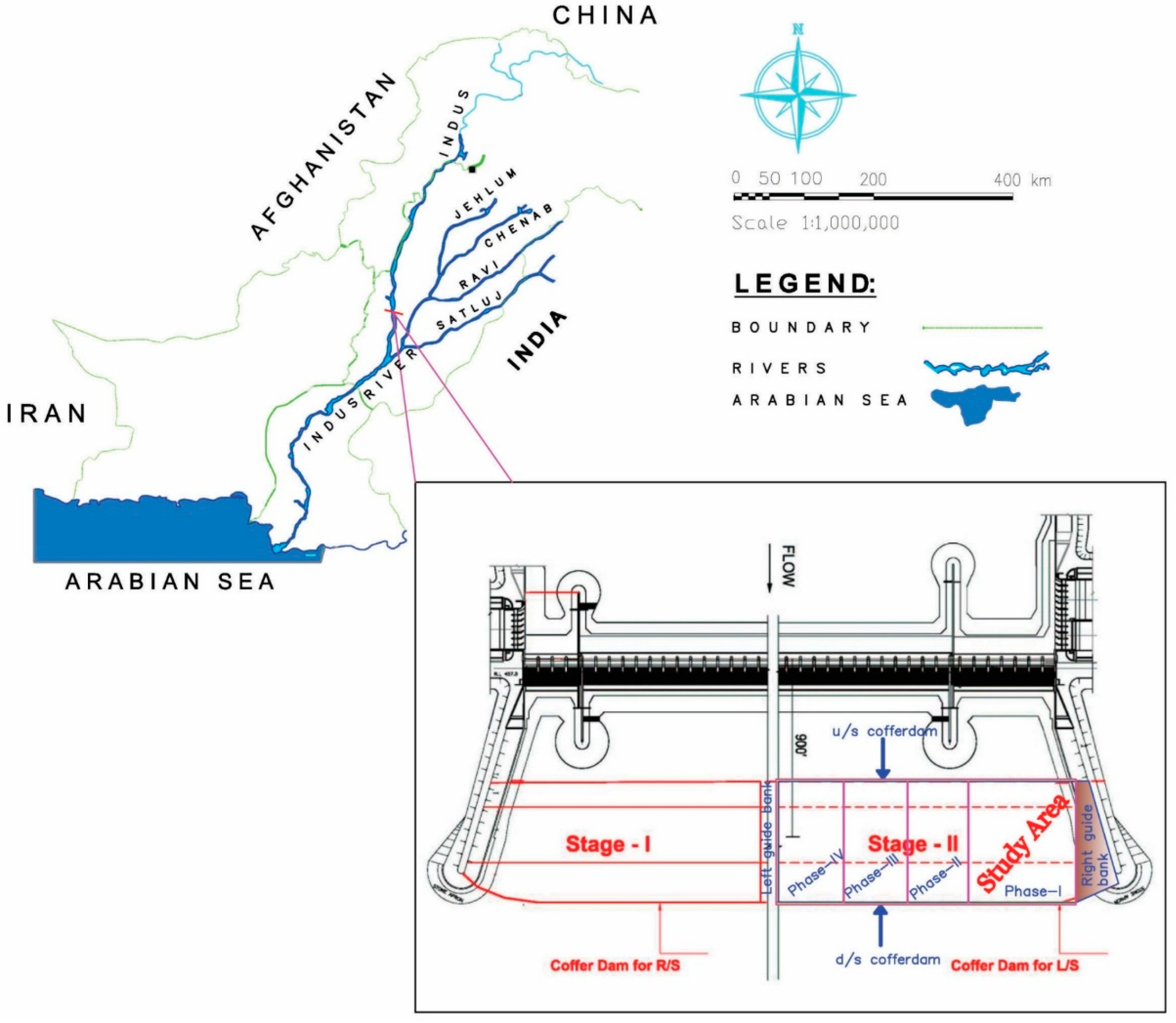
The Taunsa Barrage/Dam is located at 70°50′ E and 30°42′ N across the Indus River, which is the largest river of the Indus Valley in Pakistan. The valley is a flat alluvial fan formed by the Indus River and its tributaries. There are five main tributaries of the Indus River (Figure 1) irrigating the fertile lands of the Punjab and Sindh provinces of Pakistan. All rivers of the irrigation system of the country are interconnected through a series of link canals that facilitate interbasin water transfers. Water for irrigation is diverted from the rivers through a series of barrages (dams/diversion weirs) releasing water into main canals and subsequently to a vast irrigation network of distributaries and minor channels. The development of the irrigation system started in the middle of the 19th century when many of the existing barrages were constructed [1]. There is a major initiative from the government of Pakistan to rehabilitate the century-old infrastructure. One of these was the Taunsa Barrage, constructed in 1958 and presently feeding four main canals—two on the right and two on the left bank—irrigating a total area of 2.35 million acres [2].
Construction and rehabilitation programs of hydraulic river structures invariably involve structural activities in the riverbed, and efficient dewatering of construction sites always plays a crucial role in undisturbed structural works. The alluvial sediments, distributed in the Indus River Delta, form an unconfined aquifer of more than 300 m thickness [3,4]. Owing to this excessive aquifer thickness, along with high river water level and a deep bedrock burial depth, it is impossible to install an underground diaphragm wall down to the bedrock to provide dry conditions for construction in the riverbed. Therefore, for the projects involving structural activities in the riverbed, dewatering is widely used to reduce the groundwater level around the foundation pits; if improperly handled, however, this may cause land subsidence, geological disasters, and even major security incidents [5,6,7].
Two measures may be considered to control the groundwater flow into the foundation pits; the first measure includes the installation/construction of an underground diaphragm wall to cut off the natural groundwater flow into the foundation, and the second measure is to install pumping wells to lower the groundwater table in the foundation pits [8]. The application of diaphragm walls is limited because of high project costs and engineering difficulties. However, several researchers have adopted this measure in the projects with shallow groundwater level for controlling the water influx into the foundation pit [9,10,11,12]. The second measure of installing pumping wells has been widely used to lower the groundwater table in open pits [13,14,15], and this measure has often been used in conjunction with a diaphragm wall. Therefore, appropriate selection of relative depth of both diaphragm wall and wells plays an effective role in controlling the land subsidence outside the foundation pit.
Three-dimensional numerical simulation methods in designing the foundation pit dewatering systems have extensively been used by several researchers in recent years to provide dry conditions for construction. Luo et al. [6] used a three-dimensional finite element simulation method for foundation pit dewatering to control the groundwater level around the foundation pit, and determined that the model-simulated optimal design and the real case were consistent with each other. Alonso et al. [16] used a three-dimensional finite element approach for simulating dewatering of a construction site and found that the model accurately reproduced the observed conditions. Chen and Lei [17] applied a three-dimensional numerical simulation model for the design of a foundation pit dewatering system and concluded that the utilized method not only provided a strong basis for the optimum design of the foundation pit dewatering but also a scientific basis for decision-making related to underground construction projects.
In further studies, it is documented that an optimal design of a dewatering system may be achieved by the incorporation of groundwater flow modeling, inverse simulation studies, and optimization to minimize the total abstraction volume or execution cost, while satisfying the design criteria [18,19,20]. Zhou et al. [21] used a three-dimensional finite-difference method for simulating pit dewatering, through the inversion of hydraulic conductivity parameters, based on field pumping tests, and concluded that the predicted hydraulic head value of the three-dimensional finite-difference model is consistent with the monitored value. Ye et al. [22] developed an intelligent risk-assessment system for deep excavation dewatering, based on the coupled three-dimensional groundwater flow theory to evaluate the safety of excavation dewatering and have concluded that an increase in the insertion depth of the underground diaphragm wall will increase the water level drawdown gradually while the predicted output volume of water will decrease. Wang et al. [23] applied a three-dimensional finite-difference forward analysis approach to verify the feasibility of a dewatering scheme for a large deep foundation pit. In further studies, researchers used different techniques for dewatering of foundation pits in various regions of the world [24,25,26,27,28,29,30,31].
The characteristics of seepage in small-scale deep foundation pits of buildings or other small structures have been extensively investigated in previous studies. However, the seepage characteristics of large-scale deep foundation pits in thick aquifers (more than 300 m depth) with high water levels across a flowing river have not been studied. Therefore, this study fills this research gap. This study aims to design an optimal dewatering system for a large deep foundation pit by adopting the three-dimensional finite-difference numerical simulation approach. Under this context, the Taunsa Barrage of Pakistan was considered as a case study. Moreover, the hydraulic barrier function of an underground diaphragm wall was evaluated for selecting its optimal depth.
2. Mathematical Model
2.1. Governing Equation
The governing equation of anisotropic porous medium for three-dimensional transient groundwater flow is as follows [32]
2.1.1. Initial Condition
The initial condition of the governing equation is
2.1.2. Boundary Condition
The Dirichlet boundary condition is expressed as [32]
where, Kxx, Kyy, Kzz are the hydraulic conductivity parameters along the x, y, and z axis, respectively, and are assumed to be parallel to the traditional x-y coordinate system (LT−1); h is the piezometric head at (x, y, z) (L); W is the volumetric influx and/or efflux per unit volume of water (T−1); t is the time (T); Ss denotes the specific storage (L−1); Ω represents the computational domain; Γ1, Γ2, and Γ3 are the first, second, and phreatic surface boundaries, respectively; H0 (x, y, z, t0) represents the initial head at points (x, y, z); H1 (x, y, z, t) is the known water head at the boundary; q(x, y, z, t) represents the recharge capacity per unit area for the second type boundary condition; and nx, ny, and nz are the components of the unit normal vector on boundary Γ2 along the x, y, and z directions, respectively.
When the governing equation is combined with the initial and boundary conditions, it represents 3-D transient groundwater flow in a heterogeneous and anisotropic aquifer, given that the principal axes of hydraulic conductivity are aligned with the traditional coordinate system. Analytical solutions of such a combination of the partial differential equation are rarely available, except for very simple systems. Hence, a finite-difference numerical simulation with MODFLOW, in which the flow domain is divided into element blocks, is used to obtain an approximate solution.
2.2. Finite-Difference Solution of the Groundwater Flow Model
The solution of a finite-difference groundwater flow model follows the application of the continuity equation, that is, the summation of all inflows and outflows from each cell is equal to the change in storage, provided that the groundwater density of the considered cell is constant [33]. The balance of groundwater flow in a cell is given as follows:
where ∑Qi is the total net inflow into the cell (L3T−1); Ss denotes the aquifer specific storage; ΔV denotes the cell volume (L3); and Δh represents the piezometric head change over time Δt (T).
To account for external sources and stresses (pumping, recharge, evaporation, drainage, and river infiltration) that may affect a single cell, the combined flow equation is generally represented as:
where Qsi,j,k is the net flow into cell i, j, k from all external sources/stresses (L3T−1); hi,j,k is the piezometric head at node i, j, k; Pi,j,k is the coefficient of the head from the external stresses (L2T−1); and Qi,j,k is the flow directly injected into the cell (L3T−1).
By applying Equation (6) to cell i, j, k, also considering the six adjacent cells and their external flow rates, the resultant continuity equation may be expressed as:
where the subscript notation “1/2” denotes the volumetric flow between nodes; for example, Qi,j−1/2,k represents the volumetric flow between nodes i, j, k and i, j−1, k (L3T−1); Δrj, Δci, and Δvk are the cell dimensions along the row, column, and vertical directions (L), respectively; and ∆hi,j,k/∆t is a finite-difference approximation for the piezometric head derivation, with respect to time (LT−1), which may be expressed by the finite-difference form, as shown below:
where and are the piezometric heads at cell i, j, k at time levels m and m − 1 (L); and tm and tm−1 are times at time levels m and m − 1 (T).
According to Darcy’s Law, the finite-difference approximation of cells i, j, k may be expressed by [34].
where CR, CC, and CV represent the hydraulic conductivity between nodes i, j, k and a neighboring node (L2T−1), which may be defined as the ratio between the product of flow cross-sectional area and the coefficient of hydraulic conductivity to the length of the flow. The subscript “1/2” denotes the hydraulic conductivity between the nodes; for example, CRi,j−1/2,k describes the hydraulic conductivity between nodes i, j, k and i, j − 1, k.
Equation (10) is the finite-difference form of the continuity equation of the 3-D transient flow, which may be solved iteratively. In this equation, at the starting/initial time level (m − 1), the coefficients of the various head terms are all known. However, at the end of the time step and at time tm, the seven heads are unknown, as they are part of the head distribution that is to be predicted. Such an equation cannot be solved independently as it represents a single equation with seven unknowns. However, this kind of equation can be written for each active cell in the mesh. A system of “n” equations with “n” unknowns is formed, as only one unknown head exists for each cell. Such a system may be solved simultaneously.
3. Case Study
The Taunsa Barrage was constructed in 1958, but soon after its construction, it ran into multiple problems (e.g., the breakdown of the subsurface flow monitoring system, excessive retrogression, hydraulic jump and energy dissipation problems, excessive sedimentation, drainage problems, etc.). Therefore, its rehabilitation and modernization were planned to address the aforementioned problems.
The construction work was planned in two stages, and stage-II work was further divided into four phases to keep the barrage in operation during the entire construction period. During stage-II work, a total of 200 wells were installed and operated round the clock to achieve complete dewatering of the foundation pit. This study is limited to stage-II, phase 1 work, in which 70 wells were installed. The location of the Taunsa Barrage across the Indus River and layout of the dewatering area is presented in Figure 1.
Aquifer Hydrogeological Conditions
The main type of aquifer in the foundation pit is the unconfined aquifer of fine to medium sand of large thickness [4]. Undisturbed soil samples of riverbed material were collected and tested for the evaluation of hydraulic conductivity and profile layering. The hydraulic conductivity parameters of all the strata were obtained using a constant head permeability test [35] and by an analytical equation established by Carman [36], as follows:
where k represents the intrinsic permeability (L2), ϕ is the porosity, de is the effective particle diameter equal to d10 size (on passing basis) in particle gradation curve, K represents the hydraulic conductivity (L/T), and µ is dynamic viscosity (for water µ = 0.01 g/cm-s).
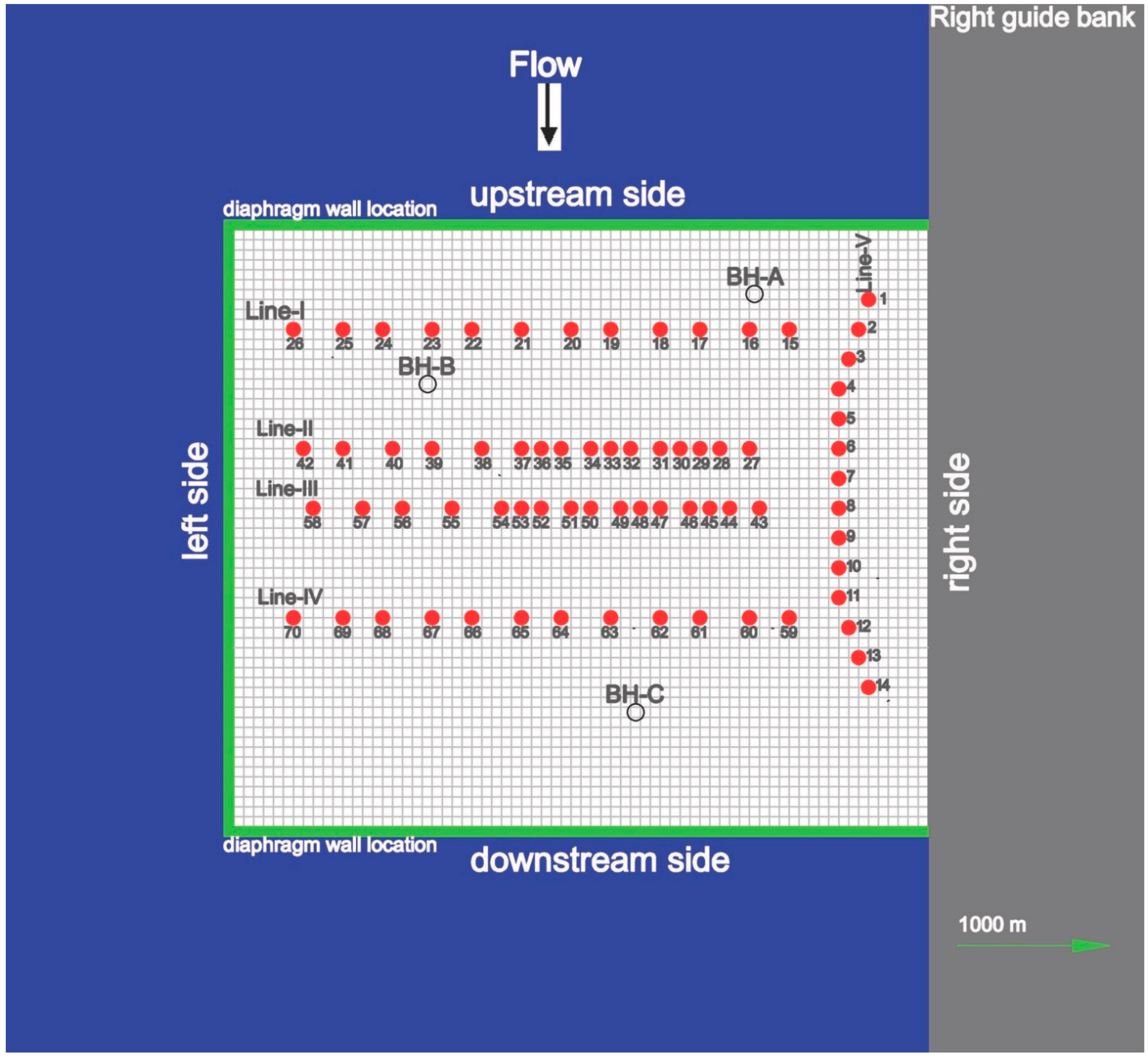
Three borehole locations, BH-A, BH-B, and BH-C (Figure 2), were selected for estimation of the hydraulic conductivity of subsoil strata, and it was found that this varies depthwise, owing to sedimentation of various-sized particles (fine to medium sand). Hydraulic conductivity of the subsurface strata, estimated by using the Kozeny–Carman equation, varies from 8.22 m/d to 11.69 m/d, while in the case of the constant head hydraulic conductivity test, it varies from 11.88 m/d to 14.46 m/d. Hydraulic conductivities at all three borehole locations, KA, KB, and KC, are listed in Table 1.
4. Numerical Model
A three-dimensional software program processing MODFLOW2000 (USGS) was adopted to simulate the dewatering system using the finite-difference method to solve the governing equation. This model was selected because it is easy to set up, free to use, and GUIs are inexpensive to run the model, though it cannot simulate the complex geological features compared to other models (e.g., FEFLOW). Also, in previous studies, several researchers [17,37,38] have employed the MODFLOW model for the design and optimization of foundation pit dewatering projects and concluded that it can simulate the dewatering systems efficiently.
4.1. Spatial Discretization and Boundary Conditions
The model covers a rectangular area of 195,040 m2 including 106 rows and 115 columns with a denser grid size of 4 × 4 m (Figure 2). Three sides of the foundation pit (upstream, left, and downstream sides) were surrounded by the river water storage throughout the construction period, and these sides were treated as constant head boundaries as the variation in the river water level was less than 1 m during the construction period. Therefore, an average river water level of 129.84 m was selected for the simulation.
On the right-hand side of the foundation pit, there is a guide bank which is almost 3 m thick from the riverbed level. Therefore, the first layer of the model on the right-hand side was treated as a no-flow boundary, while in the remaining layers, a constant head boundary equal to 125.92 m was assigned 1000 m away from the system, to minimize the effect of the radius of influence. The plan view of the dewatering area, with the location of the underground diaphragm wall and the layout of the pumping wells, is presented in Figure 2.
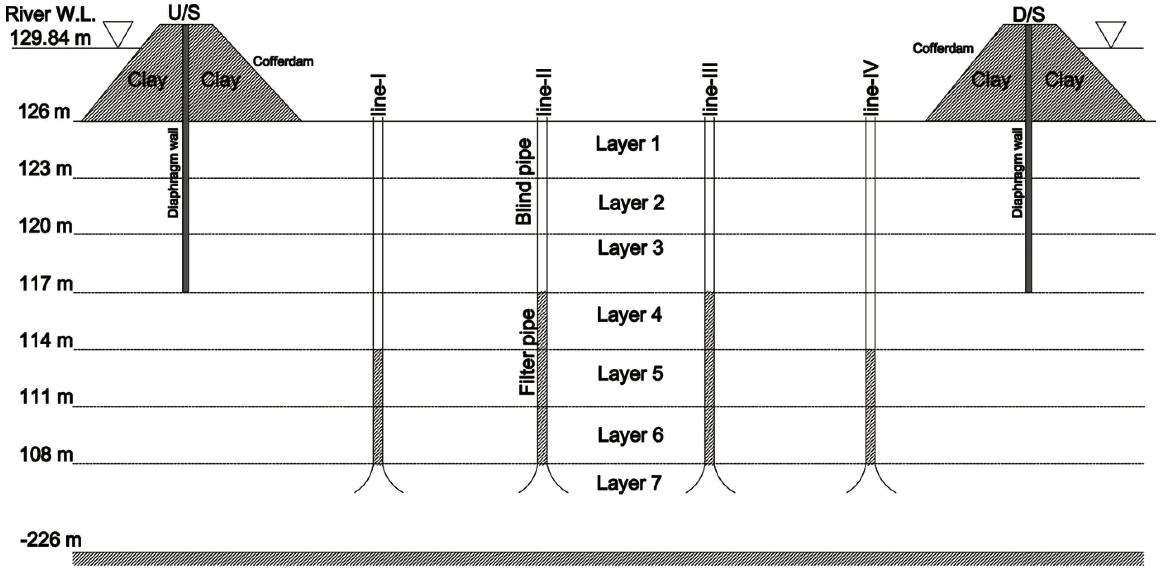
In the vertical direction, 18 m aquifer thickness below the riverbed was considered on the basis of strata distribution and was divided into six layers, each of which was 3 m thick, and an additional seventh layer was added at the same bottom plate level as that of the bedrock of the actual aquifer, which was about 300 m thick below the riverbed level [3,4], and was defined as the impermeable boundary. The filters of the pumping wells were set between 108 m and 117 m for line-II, line-III, and line-V wells, while for line-I and line-IV wells, the filter pipe length was between 108 m and 114 m. The depth of the underground diaphragm wall was selected 9 m below the riverbed level for calibration purpose, while for the optimal selection of its depth, different schemes were developed, which are discussed in Section 5. Figure 3 shows the cross-sectional view of the foundation pit, cofferdam location, underground diaphragm wall location, locations of pumping well lines, and the thickness of layers. The conductivity through the joints of the metallic diaphragm wall was considered as 1 × 10⁻¹⁰ m/s [39,40,41], and inserted down to the level of 117 m (layers 1–3). The hydraulic conductivity parameters of all the strata in the calculation range are listed in Table 1.
4.2. Model Identification and Calibration
As per model requirements, time variant and invariant data were used for the model formulation. Time variant data includes the details of pumping wells, which were specified in the model for the whole dewatering period based on the observed strata distribution and actual on-site pumping (well locations, pumping rate, and pumping duration) carried out during the construction period. The length of each stress period was 1 day. The pumping capacities of all the installed wells were assigned to the model based on daily pumping status and according to their contribution in specific layers (Figure 3). The capacity of each well is shown in Table 2. Time invariant parameters include aquifer data (i.e., horizontal and vertical distribution of subsurface strata, aquifer thickness, porosity, specific yield, specific storage, layer properties (confined/unconfined), etc.). The calculated hydraulic conductivity values were first assigned and then revised by fitting the calculated hydraulic heads to the observed heads. The model-calculated hydraulic conductivity parameters of the riverbed strata are presented in Table 3.
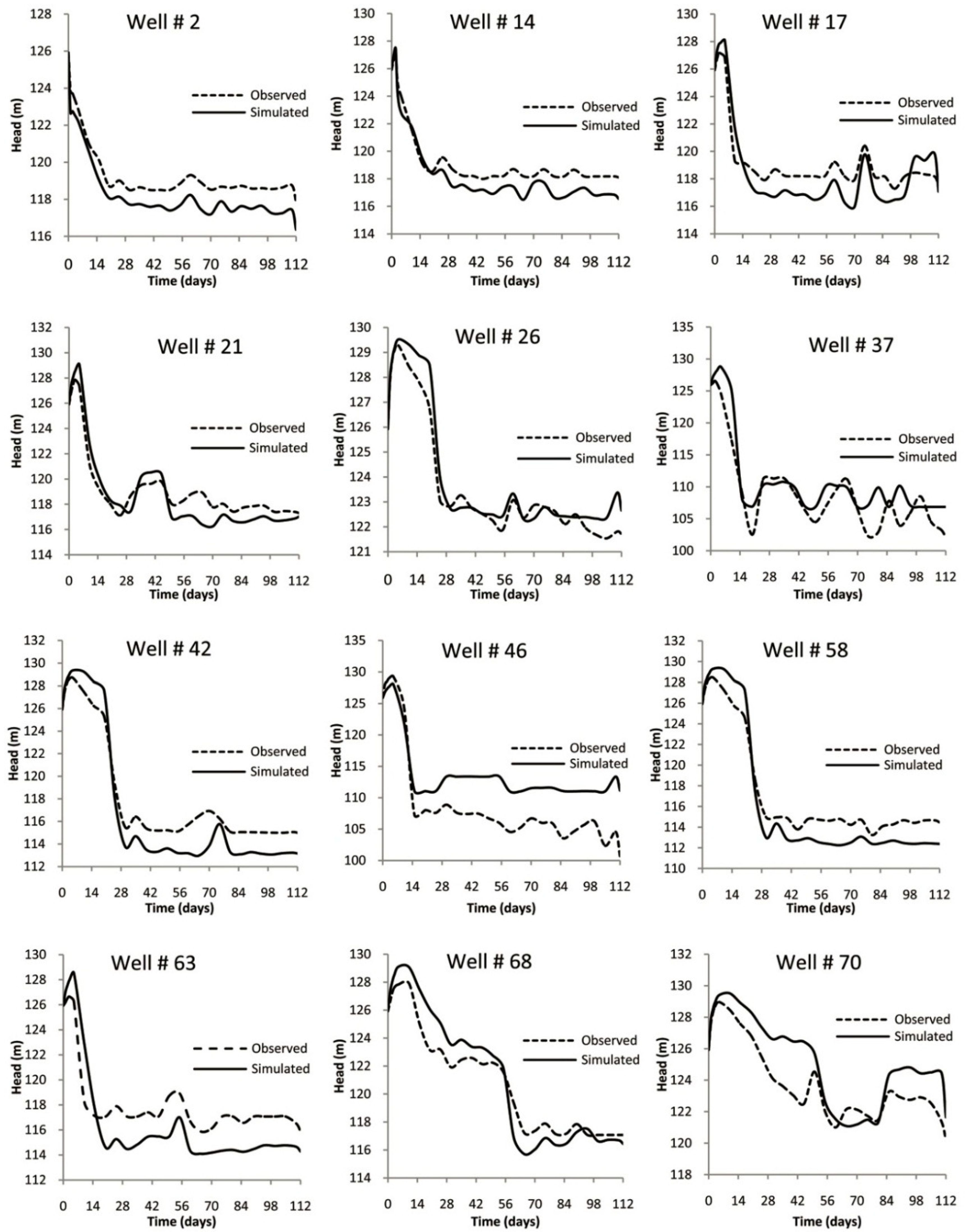
A total of 70 wells were installed for complete dewatering of the construction area, out of which 12 wells were selected for model calibration. As shown in Figure 2, wells installed in line-I (W-15 to W-26), line-IV (W-59 to W-70), and line-V (W-1 to W-14) control the underground seepage influx from the upstream, downstream, and the right-hand side of the foundation pit, respectively, whereas wells W-26, W-42, W-58, and W-70 control the inflow from the left-hand side of river water storage.
The model-simulated water levels were plotted and compared with the field-observed water levels for the whole dewatering period, which was 112 days. The model was calibrated with the field-observed conditions by adjusting the hydrological parameters. Figure 4 shows the comparison between the observed and computed heads for 12 wells. As shown in Figure 4, a steady water level was not achieved in well W-70, as it was influenced by the inflows from two sides of the river boundary (d/s side and left side), and also as a result of the fluctuations of its daily operational status. The simulation results indicate that the calculated water levels were comparable with the observed data. After 20–25 days of pumping, a pseudosteady condition was attained, and the water level in the foundation pit fell to 117.92 m, which was below the targeted value.
4.3. Error Analysis
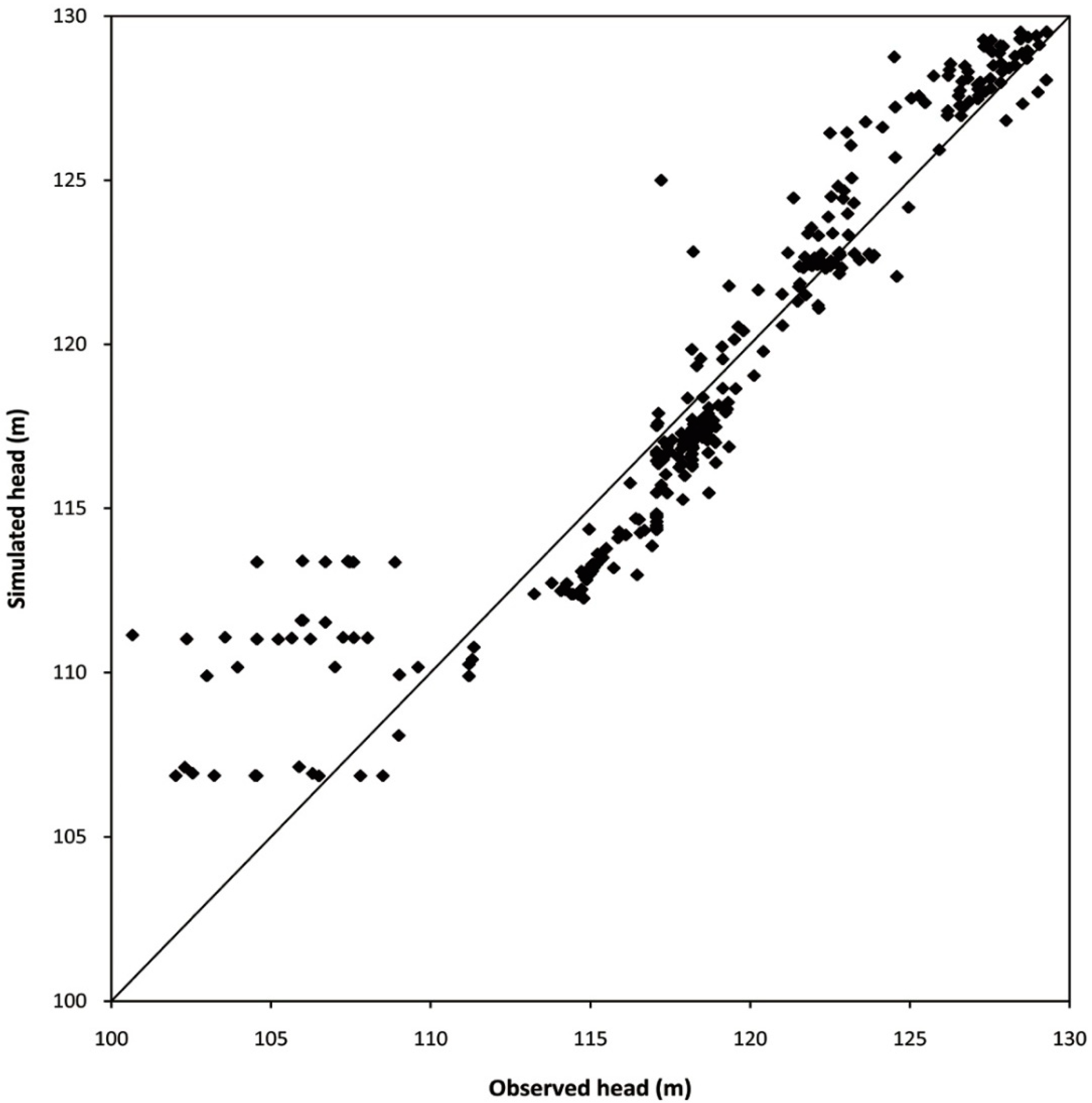
After model calibration, the error was analyzed and a mean root-mean-square error (RMSE) of 1.46 m was found in the model-fitted heads to observations, against an average head drop of about 10.5 meters (Figure 5). In previous studies, several researchers [7,21,23,30] have found error ranges from 7.6 to 30.8 percent in the calibration of three-dimensional groundwater numerical models. In the present study, an error of 11.7% (RMSE/∆h) was found when the model-simulated water levels were equal to or less than the observed ones, whereas an average error of 13.9 percent (RMSE/∆h) was observed. These errors may be associated with the variations in the hydraulic conductivity, which was assumed constant throughout the simulation period. Therefore, these errors may be accepted considering the complexity of the system.
5. Dewatering System Optimization
Different schemes and scenarios, discussed in the subsequent sections, were developed to determine the optimal depth of the diaphragm wall and to estimate the impact of hydraulic conductivity on the dewatering system performance, and are discussed in the subsequent sections.
5.1. Selection of Diaphragm Wall Depth
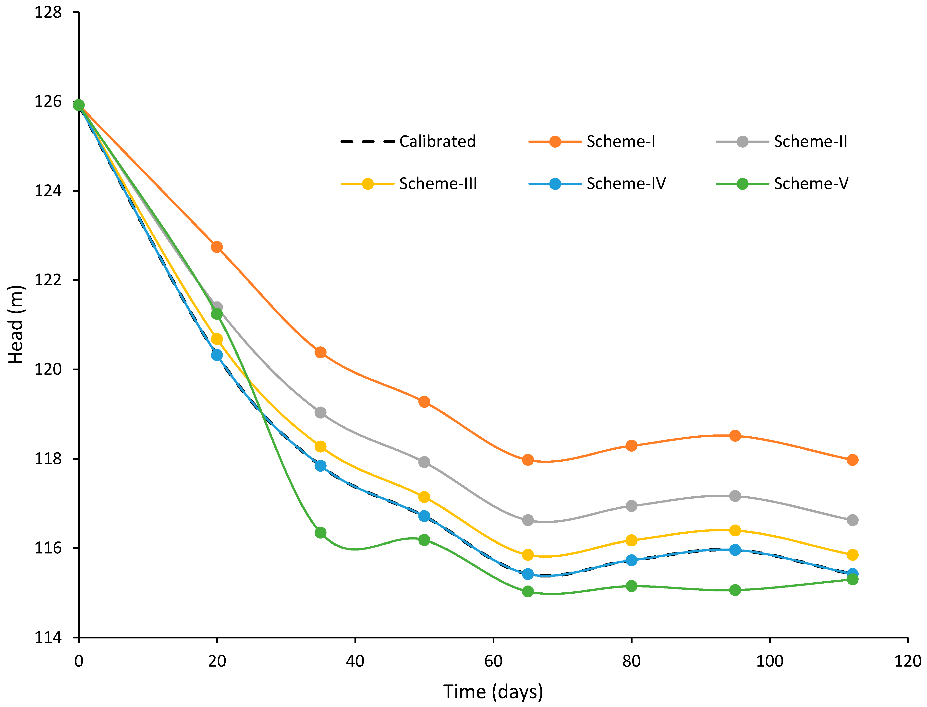
In order to select the optimal insertion depth of the underground diaphragm wall, different schemes have been developed by adjusting its bottom level, for analyzing its impact on the dewatering system. The simulation results of these schemes are presented in Table 4 and Figure 6 and are briefly discussed below.
5.1.1. Scheme-I
In this scheme, the depth of the underground diaphragm wall was not adjusted, and its bottom level was same as that of the riverbed level. The bottom of the filter pipe of all the pumping wells was 18 m below the level of the underground diaphragm wall. The simulation results of scheme-I, presented in Table 4 and Figure 6, showed that with these settings, an average water level of 120.13 m may be attained, which cannot satisfy the dewatering requirements, as the targeted water level was 119.78 m. Therefore, these arrangements for a dewatering system are not acceptable, as they are unable to achieve the required water level to provide dry conditions for undisturbed construction work, and may also cause serious stability and environmental issues [5,6,7].
5.1.2. Scheme-II
In this scheme, the depth of the underground diaphragm wall was increased to 3 m below the riverbed level and bottom of the filter pipe of pumping wells was kept 15 m below the bottom level of the diaphragm wall. The simulated water level was 1.18 m below the water level compared to the previous scheme, as shown in Table 4. With these settings of the underground diaphragm wall, the attained water level was 118.95 m, which may satisfy the dewatering requirements. However, the settings of the level of the diaphragm wall, in this case, may result in serious stability problems, and the filter pipe of pumping wells may also be exposed, which might cause excessive drawdown outside the foundation pit, and at the same time, induce other environmental and geological issues. Therefore, these settings of the bottom level of the underground diaphragm wall cannot be adopted.
5.1.3. Scheme-III
Like scheme-II, a third scheme was developed, but in this case, the depth of the underground diaphragm wall was increased to 6 m below the riverbed level. As shown in Table 4, the attained water level with these conditions was 118.28 m, which was 0.67 m below the water level achieved in scheme-II and 1.50 m below the target value. The drawdown outside the foundation pit was also not more than 1 m. Hence, with this level of underground diaphragm wall, the dewatering requirements may be satisfied successfully, and environmental and geological issues would be minimal. However, in this case, the simulated and observed results are not comparable, as the selected depth of the underground diaphragm wall was 9 m below the riverbed level during the construction project.
5.1.4. Scheme-IV
In scheme-IV, the depth of the underground diaphragm wall was extended to 9 m below the riverbed level. As shown in Table 4, the water level in this scheme was lowered to 117.92 m, which was 1.86 m below the required water level. At this level of the underground diaphragm wall, the observed and simulated water levels were comparable (Figure 4). The insertion of the diaphragm wall up to this level results in a 2.21 m lowered water level, compared to that if no diaphragm wall is installed. Therefore, the insertion of the diaphragm wall reduces the dewatering effort significantly.
5.1.5. Scheme-V
To evaluate the impact of the depth of the diaphragm wall, an additional scheme was developed. In scheme-V, the depth of the underground diaphragm wall was increased to 18 m below the riverbed level; the bottom of the filter pipe was at the same level as that of the diaphragm wall level. In this case, when the depth of the underground diaphragm wall was increased from 9 m to 18 m below the riverbed level, it only resulted in a 0.39 m drawdown, whereas a drawdown value of 2.21 m was obtained when the bottom level of the diaphragm wall adjusted from 0 to 9 m below the riverbed level. Therefore, any further increase in the depth of the underground diaphragm wall from 9 m will yield small variations in the simulated water levels.
5.2. Hydraulic Conductivity Variation
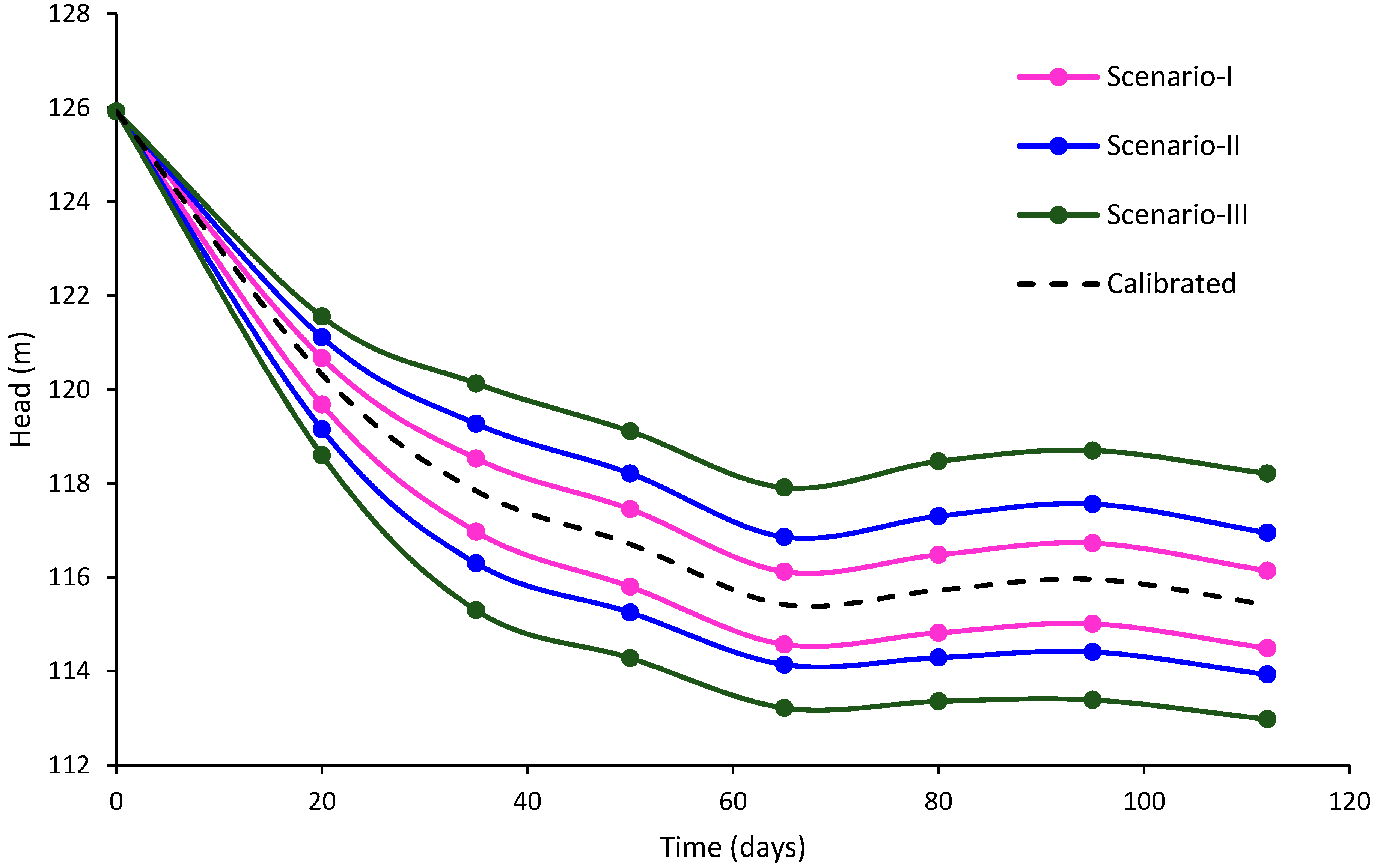
After calibration, the model was tested by varying the values of hydraulic conductivity (both Kh and Kv) to assess its impact on the dewatering system and to evaluate model applicability with different subsurface strata types. Three scenarios were developed by varying the values of K, and the simulation results are presented in Table 5 and Figure 7.
5.2.1. Scenario-I
In scenario-I, the model was simulated with a 10% increased and decreased value of hydraulic conductivity of subsurface strata from those of the calibrated values of K. The other parameters of the model were kept the same as those of the calibrated model. The simulation results, presented in Table 5 and Figure 7, showed that when the value of hydraulic conductivity was increased by 10%, the attained average water level was 118.50, which was 0.59 m higher than that of the calibrated value of 117.92 m. Similarly, when the value of K was decreased by 10%, the simulated average water level was 117.16 m, which was 0.76 m lower than the calibrated value of the water level.
5.2.2. Scenario-II
In this scenario, the value of hydraulic conductivity varied by 20% from the model-calibrated K value. When the value of hydraulic conductivity of subsoil strata was increased by 20%, the resulted average simulated water level was 119.15 m, which was 1.23 m higher than that of the calibrated value, while a decrease in the K value resulted in a 1.24 m lower water level, as compared to the model-calibrated water level.
5.2.3. Scenario-III
Similar to previous scenarios, a third scenario was developed by a 30% variation in the hydraulic permeability parameters from the calibrated K. In this case, an increase in the value of hydraulic conductivity resulted in a 2.09 m higher water table, as compared to calibrated results. Conversely, when the K values were lowered, the simulated water level was about 115.88 m, which was about 2.04 m lower than that of the calibrated water level, as shown in Table 5.
6. Discussion
The proposed method of dewatering system design in this study gives an insight into the coupling effect among the underground diaphragm wall, seepage influx into the foundation pit, and the hydraulic properties of subsoil strata. A three-dimensional numerical simulation model, MODFLOW, was used to design the dewatering system at a large deep foundation pit at the Taunsa Barrage, to demonstrate its applicability. The hydraulic conductivity of the subsurface strata obtained by laboratory tests was used as the initial conditions for the model, which was then revised during model calibration [23]. The model-calibrated results were comparable with field-observed water level in the foundation pit and found consistent with previous studies by several researchers [17,23,38,42,43] in which they have used three-dimensional numerical simulation methods for dewatering of foundation pits in different regions of the world. Once the model was successfully calibrated, different schemes and scenarios were developed for the selection of the optimal depth of the underground diaphragm wall and to evaluate the impact of hydraulic conductivity parameters on the dewatering system, respectively.
Five schemes for the selection of optimal depth of diaphragm wall were discussed in this article. In scheme-I, the simulated water level was unable to satisfy the dewatering requirements, and at the same time, it may also cause serious foundation stability and environmental and geological problems [5,7]. Schemes II–V met the dewatering requirements, as the simulated water level in these schemes was below the targeted level to provide dry conditions for undisturbed construction work. However, scheme-II may cause stability and environmental issues, whereas an optimal design of the dewatering system may be developed by scheme-IV. During the construction, selected depth of the selected underground diaphragm wall was 9 m below the riverbed level, which was addressed in scheme-IV. Installation of the underground diaphragm wall drastically reduced the dewatering effort and provided stability to the foundation pit. The difference in the drawdown was decreased by increasing the depth of the underground diaphragm wall. Therefore, an optimal selection of the depth of the underground diaphragm wall is obligatory prior to construction work, as it involves high economic cost.
The results of the three-dimensional numerical simulation model revealed that the number of pumping wells affects the water level in the foundation pit. The greater the number of wells, the stronger the pumping capacity, but this will increase construction costs. Conversely, the smaller the number of wells, the more the pumping capacity decreases, but there are cost savings. Thus, numerical simulation of the dewatering system prior to construction should be performed to analyze the performance of a dewatering system under different geological and hydrological conditions.
7. Conclusions
This study analyzed the performance of the dewatering system in a large deep foundation pit by using finite-difference numerical simulations. In most of the dewatering projects, the major unknown parameter is the hydraulic conductivity, thus a three-dimensional finite-difference numerical model was employed to revise the hydraulic conductivity parameters obtained from laboratory tests. The adopted hydraulic conductivity parameter for the calibration was slightly less than the median hydraulic conductivity obtained by using the Kozeny–Carman equation and constant head permeability test methods.
The results of the three-dimensional numerical simulation model revealed that when the depth of the underground diaphragm wall is not adjusted (i.e., its bottom level is considered the same as the riverbed level), it cannot meet the dewatering requirements and may induce foundation stability and environmental problems. Different schemes were developed for the selection of optimal depth of the underground diaphragm wall by varying its bottom level below the riverbed and the results revealed that the installation of the underground diaphragm wall can effectively increase the drawdown in the foundation pit to meet the dewatering requirements. Optimal depth of the underground diaphragm wall was attained at 9 m below the riverbed level and it was noted that any further increase in the depth of the underground diaphragm wall from 9 m resulted in insignificant variations in the simulated water levels. The model was tested to assess the impact of hydraulic conductivity on the dewatering system performance by varying the calibrated value of hydraulic conductivity, and it is concluded that the pumping rate of the dewatering system is directly proportional to the coefficient of hydraulic conductivity of subsurface strata, and therefore needs to be determined reasonably accurately prior to any dewatering system design.
There are some limitations of this study that need to be addressed further. Firstly, no economic analysis has been done in this study to calculate the total economic value that may be saved by the optimal selection of the depth of the underground diaphragm wall. Secondly, the selection of the number of wells for the optimal design of the dewatering system needs to be addressed, as during this dewatering project, the attained water levels were 2 to 3 m lower than the targeted water levels.
Author Contributions
Conceptualization, I.A. and X.D.; Methodology, I.A. and M.T.; Software, I.A. and M.Z.; Validation, M.T., M.Z. and M.N.A.; Formal Analysis, I.A. and M.T.; Investigation, I.A.; Resources, X.D.; Data Curation, I.A.; Writing-Original Draft Preparation, I.A.; Writing-Review & Editing, M.N.A; Visualization, M.T.; Supervision, X.D.; Project Administration, X.D.; Funding Acquisition, X.D.
Funding
This study was funded by the State Key Program of National Natural Science of China (51239004), the National Natural Science Foundation of China (51309105, 40701024), and the Power Construction Corporation of China (DJ-ZDZX-2016-02).
Acknowledgments
This study was supported by the State Key Program of National Natural Science of China (51239004), the National Natural Science Foundation of China (51309105, 40701024), and the Power Construction Corporation of China (DJ-ZDZX-2016-02). Ijaz Ahmad and Muhammad Tayyab contributed equally in this research.
Conflicts of Interest
The authors declare no conflict of interest.
References
Gulick, L.H. Irrigation Systems of the Former Sind Province, West Pakistan. Geogr. Rev.1963, 53, 79. [Google Scholar] [CrossRef]
Zaidi, S.M.A.; Amin, M.; Ahmadani, M.A. Performance evaluation of Taunsa barrage emergency rehabilitation and modernization project. In Proceedings of the 71st Annual Session Proceedings Pakistan Engineering Congress, Karachi, Pakistan, 26–30 July 2011; pp. 650–682. [Google Scholar]
Basharat, M.; Rizvi, S.A. Groundwater extraction and waste water disposal regulation—Is lahore aquifer at stake with as usual approach. In Proceedings of the Pakistan Engineering Congress, Karachi, Pakistan, 26–30 July 2011; pp. 135–152. [Google Scholar]
Basharat, M. Spatial and temporal appraisal of groundwater depth and quality in LBDC Command-Issues and Options. Pak. J. Engg. Appl. Sci2012, 11, 14–29. [Google Scholar]
Hsi, J.P.; Carter, J.P.; Small, J.C. Surface subsidence and drawdown of the water table due to pumping. Development1994, 44, 381–396. [Google Scholar] [CrossRef]
Luo, Z.; Zhang, Y.; Wu, Y. Finite element numerical simulation of three-dimensional seepage control for deep foundation pit dewatering. J. Hydrodyn. Ser. B2008, 20, 596–602. [Google Scholar] [CrossRef]
Wang, J.; Feng, B.; Liu, Y.; Wu, L.; Zhu, Y.; Zhang, X.; Tang, Y.; Yang, P. Controlling subsidence caused by de-watering in a deep foundation pit. Bull. Eng. Geol. Environ.2012, 71, 545–555. [Google Scholar] [CrossRef]
Younger, P.L.; Robins, N.S. Challenges in the characterization and prediction of the hydrogeology and geochemistry of mined ground. Geol. Soc. Lond. Spec. Publ.2002, 198, 1–16. [Google Scholar] [CrossRef]
Jiang, S.; Kong, X.; Ye, H.; Zhou, N. Groundwater dewatering optimization in the Shengli no. 1 open-pit coalmine, Inner Mongolia, China. Environ. Earth Sci.2013, 69, 187–196. [Google Scholar] [CrossRef]
Wang, J.; Hu, L.; Wu, L.; Tang, Y.; Zhu, Y.; Yang, P. Hydraulic barrier function of the underground continuous concrete wall in the pit of subway station and its optimization. Environ. Geol.2009, 57, 447–453. [Google Scholar] [CrossRef]
Xu, Y.S.; Shen, S.L.; Ma, L.; Sun, W.J.; Yin, Z.Y. Evaluation of the blocking effect of retaining walls on groundwater seepage in aquifers with different insertion depths. Eng. Geol.2014, 183, 254–264. [Google Scholar] [CrossRef]
Wu, Y.-X.; Shen, S.-L.; Wu, H.-N.; Xu, Y.-S.; Yin, Z.-Y.; Sun, W.-J. Environmental protection using dewatering technology in a deep confined aquifer beneath a shallow aquifer. Eng. Geol.2015, 196, 59–70. [Google Scholar] [CrossRef]
Mahmoud, H.; Elghany, A.; Ahmed, A. Optimization for number of vertical drainage wells in highly heterogenious aquifers. Int. J. Multidiscip. Res. Rev.2015, 2, 569–582. [Google Scholar]
Wang, J.; Huang, T.; Sui, D. A case study on stratified settlement and rebound characteristics due to dewatering in shanghai subway station. Sci. World J.2013, 2013. [Google Scholar] [CrossRef]
Xu, B.; Yan, C.; Sun, Q.; Liu, Y.; Hou, J.; Liu, S.; Che, C. Field pumping experiments and numerical simulations of shield tunnel dewatering under the Yangtze River. Environ. Earth Sci.2016, 75, 715. [Google Scholar] [CrossRef]
Alonso, C.; Ferrer, A.; Soria, V. Finite element simulation of construction site dewatering. In Proceedings of the International Conference on Engineering and Mathematics ENMA 2008, Bilbao, Spain, 7–9 July 2008. [Google Scholar]
Chen, G.X.; Lei, W. Application 3D numerical simulation on foundation pit dewatering design of nanchang international financial center. Adv. Mater. Res.2010, 108, 1482–1485. [Google Scholar] [CrossRef]
Demirbaş, K.; Altan-Sakarya, A.B.; Önder, H. Optimal dewatering of an excavation site. In Proceedings of the Institution of Civil Engineers-Water Management; Thomas Telford Ltd.: London, UK, 2012; Volume 165, pp. 327–337. [Google Scholar]
Roy, D.; Robinson, K.E. Surface settlements at a soft soil site due to bedrock dewatering. Eng. Geol.2009, 107, 109–117. [Google Scholar] [CrossRef]
Tokgoz, M.; Yilmaz, K.K.; Yazicigil, H. Optimal aquifer dewatering schemes for excavation of collector line. J. Water Resour. Plan. Manag.2002, 128, 248–261. [Google Scholar] [CrossRef]
Zhou, N.; Vermeer, P.A.; Lou, R.; Tang, Y.; Jiang, S. Numerical simulation of deep foundation pit dewatering and optimization of controlling land subsidence. Eng. Geol.2010, 114, 251–260. [Google Scholar] [CrossRef]
Ye, X.W.; Ran, L.; Yi, T.H.; Dong, X.B. Intelligent risk assessment for dewatering of metro-tunnel deep excavations. Math. Probl. Eng.2012, 2012, 618979. [Google Scholar] [CrossRef]
Wang, J.; Feng, B.; Yu, H.; Guo, T.; Yang, G.; Tang, J. Numerical study of dewatering in a large deep foundation pit. Environ. Earth Sci.2013, 69, 863–872. [Google Scholar] [CrossRef]
Geravandi, E.; Kamanbedast, A.A.; Masjedi, A.R.; Heidarnejad, M.; Bordbar, A. Laboratory Investigation of The Impact of Armor Dike Simple and L-Shaped in Upstream and Downstream Intake of the Hydraulic Flow of the Kheirabad River to Help Physical Model. Fresenius Environ. Bull.2018, 27, 263–276. [Google Scholar]
Yihdego, Y.; Danis, C.; Paffard, A.; Yihdego, Y.; Danis, C.; Paffard, A. Groundwater Engineering in an Environmentally Sensitive Urban Area: Assessment, Landuse Change/Infrastructure Impacts and Mitigation Measures. Hydrology2017, 4, 37. [Google Scholar] [CrossRef]
Gao, D.; Liu, Y.; Wang, T.; Wang, D.; Gao, D.; Liu, Y.; Wang, T.; Wang, D. Experimental Investigation of the Impact of Coal Fines Migration on Coal Core Water Flooding. Sustainability2018, 10, 4102. [Google Scholar] [CrossRef]
Ma, X.; Fan, Y.; Dong, X.; Chen, R.; Li, H.; Sun, D.; Yao, S.; Ma, X.; Fan, Y.; Dong, X.; et al. Impact of Clay Minerals on the Dewatering of Coal Slurry: An Experimental and Molecular-Simulation Study. Minerals2018, 8, 400. [Google Scholar] [CrossRef]
Vukelić, Ž.; Dervarič, E.; Šporin, J.; Vižintin, G.; Vukelić, Ž.; Dervarič, E.; Šporin, J.; Vižintin, G. The Development of Dewatering Predictions of the Velenje Coalmine. Energies2016, 9, 702. [Google Scholar] [CrossRef]
Guo, X.; Sun, X.; Ma, J. Numerical Simulation of Three-dimensional Soil Water Content Distribution in Water Storage Pit Irrigation. Fresenius Environ. Bull.2018, 27, 7390–7400. [Google Scholar]
Sege, J.; Wang, C.; Li, Y.; Chang, C.-F.; Chen, J.; Chen, Z.; Osorio-Murillo, C.A.; Zhu, H.; Rubin, Y.; Li, X. Modeling water table drawdown and recovery during tunnel excavation in fractured rock. In AGU Fall Meeting Abstracts; American Geophysical Union: San Francisco, CA, USA, 2015. [Google Scholar]
You, Y.; Yan, C.; Xu, B.; Liu, S.; Che, C. Optimization of dewatering schemes for a deep foundation pit near the Yangtze River, China. J. Rock Mech. Geotechnol. Eng.2018, 10, 555–566. [Google Scholar] [CrossRef]
Wu, J.; Xue, Y. Groundwater Dynamics; China Water and Power Press: Beijing, China, 2009.
McDonald, M.G.; Harbaugh, A.W. A Modular Three-Dimensional Finite-Difference Ground-Water Flow Model; US Geological Survey: Reston, VA, USA, 1988.
Harbaugh, A.W.; Banta, E.R.; Hill, M.C.; Mcdonald, M.G.; Groat, C.G. MODFLOW-2000, The U.S. Geological Survey Modular Groundwater Model User Guide to Modularization Concepts and the Groundwater Flow Process; U.S. Geological Survey, Open-File Report 00-92; U.S. Department of the Interior: Washington, DC, USA, 2000.
Head, K.H.; Epps, R. Manual of Soil Laboratory Testing; Pentech Press London: London, UK, 1986; Volume 3. [Google Scholar]
Mohan, S.; Sreejith, P.K.; Pramada, S.K. Optimization of open-pit mine depressurization system using simulated annealing technique. J. Hydraul. Eng.2007, 133, 825–830. [Google Scholar] [CrossRef]
Zaidel, J.; Markham, B.; Bleiker, D. Simulating seepage into mine shafts and tunnels with MODFLOW. Ground Water2010, 48, 390–400. [Google Scholar] [CrossRef]
Shoji, Y.; Kumeda, M.; Tomita, Y. Experiments on Seepage through Interlocking Joints of Sheet Pile, Report of the Port and Harbour Institute; Nagase: Yokosuka, Japan, 1982; Volume 21. [Google Scholar]
Fell, R.; MacGregor, P.; Stapledon, D. Geotechnical Engineering of Embankment Dams; Balkema: Park City, UT, USA, 1992; ISBN 9054101288. [Google Scholar]
Sellmeijer, J.B.; Cools, J.; Decker, J.; Post, W.J. Hydraulic resistance of steel sheet pile joints. J. Geotechnol. Eng.1995, 121, 105–110. [Google Scholar] [CrossRef]
Omer, J.R. Integrating finite element and load-transfer analyses in modelling the effects of dewatering on pile settlement behaviour. Can. Geotechnol. J.2012, 49, 512–521. [Google Scholar] [CrossRef]
Wang, J.; Feng, B.; Guo, T.; Wu, L.; Lou, R.; Zhou, Z. Using partial penetrating wells and curtains to lower the water level of confined aquifer of gravel. Eng. Geol.2013, 161, 16–25. [Google Scholar] [CrossRef]
Figure 1.
Location of Taunsa Barrage and layout of dewatering area.
Figure 1.
Location of Taunsa Barrage and layout of dewatering area.
Figure 2.
Plan view of the construction area.
Figure 2.
Plan view of the construction area.
Figure 3.
Cross-sectional view of the construction area.
Figure 3.
Cross-sectional view of the construction area.
Figure 4.
Fitting curves in the revised parameter model.
Figure 4.
Fitting curves in the revised parameter model.
Figure 5.
Error analysis in the revised parameter model.
Figure 5.
Error analysis in the revised parameter model.
Figure 6.
Fitting curves based on different depths of underground diaphragm wall.
Figure 6.
Fitting curves based on different depths of underground diaphragm wall.
Figure 7.
Fitting curves based on hydraulic conductivity variation.
Figure 7.
Fitting curves based on hydraulic conductivity variation.
Ahmad, I.; Tayyab, M.; Zaman, M.; Anjum, M.N.; Dong, X.
Finite-Difference Numerical Simulation of Dewatering System in a Large Deep Foundation Pit at Taunsa Barrage, Pakistan. Sustainability2019, 11, 694.
https://doi.org/10.3390/su11030694
AMA Style
Ahmad I, Tayyab M, Zaman M, Anjum MN, Dong X.
Finite-Difference Numerical Simulation of Dewatering System in a Large Deep Foundation Pit at Taunsa Barrage, Pakistan. Sustainability. 2019; 11(3):694.
https://doi.org/10.3390/su11030694
Chicago/Turabian Style
Ahmad, Ijaz, Muhammad Tayyab, Muhammad Zaman, Muhammad Naveed Anjum, and Xiaohua Dong.
2019. "Finite-Difference Numerical Simulation of Dewatering System in a Large Deep Foundation Pit at Taunsa Barrage, Pakistan" Sustainability 11, no. 3: 694.
https://doi.org/10.3390/su11030694
APA Style
Ahmad, I., Tayyab, M., Zaman, M., Anjum, M. N., & Dong, X.
(2019). Finite-Difference Numerical Simulation of Dewatering System in a Large Deep Foundation Pit at Taunsa Barrage, Pakistan. Sustainability, 11(3), 694.
https://doi.org/10.3390/su11030694
Note that from the first issue of 2016, this journal uses article numbers instead of page numbers. See further details here.
Article Metrics
No
No
Article Access Statistics
For more information on the journal statistics, click here.
Multiple requests from the same IP address are counted as one view.
Ahmad, I.; Tayyab, M.; Zaman, M.; Anjum, M.N.; Dong, X.
Finite-Difference Numerical Simulation of Dewatering System in a Large Deep Foundation Pit at Taunsa Barrage, Pakistan. Sustainability2019, 11, 694.
https://doi.org/10.3390/su11030694
AMA Style
Ahmad I, Tayyab M, Zaman M, Anjum MN, Dong X.
Finite-Difference Numerical Simulation of Dewatering System in a Large Deep Foundation Pit at Taunsa Barrage, Pakistan. Sustainability. 2019; 11(3):694.
https://doi.org/10.3390/su11030694
Chicago/Turabian Style
Ahmad, Ijaz, Muhammad Tayyab, Muhammad Zaman, Muhammad Naveed Anjum, and Xiaohua Dong.
2019. "Finite-Difference Numerical Simulation of Dewatering System in a Large Deep Foundation Pit at Taunsa Barrage, Pakistan" Sustainability 11, no. 3: 694.
https://doi.org/10.3390/su11030694
APA Style
Ahmad, I., Tayyab, M., Zaman, M., Anjum, M. N., & Dong, X.
(2019). Finite-Difference Numerical Simulation of Dewatering System in a Large Deep Foundation Pit at Taunsa Barrage, Pakistan. Sustainability, 11(3), 694.
https://doi.org/10.3390/su11030694
Note that from the first issue of 2016, this journal uses article numbers instead of page numbers. See further details here.

 ,
, 


