Short-Term Wind Speed Forecasting Based on Hybrid Variational Mode Decomposition and Least Squares Support Vector Machine Optimized by Bat Algorithm Model

Abstract
1. Introduction
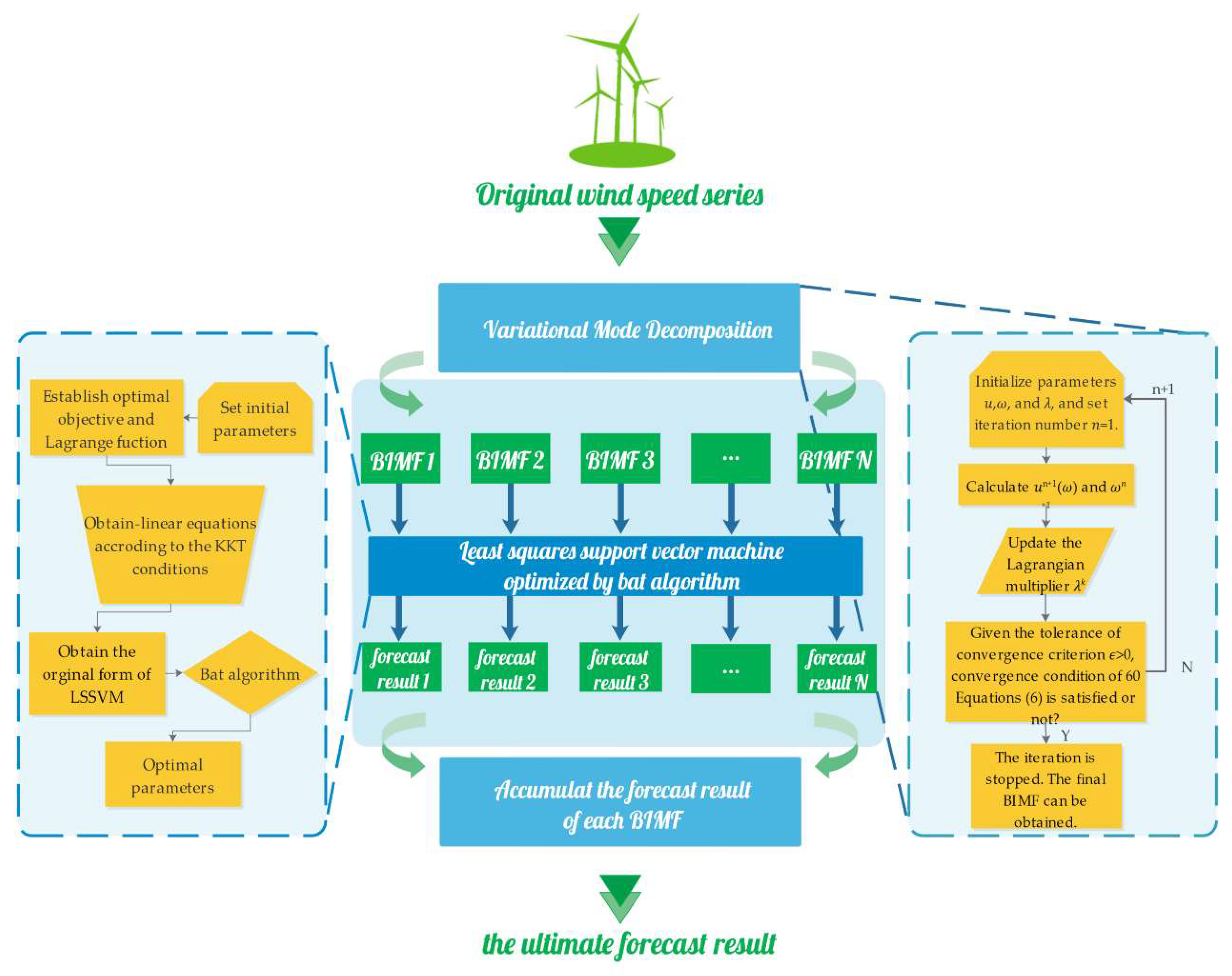
2. Methods
2.1. Variational Mode Decomposition
2.2. Ensemble Empirical Mode Decomposition
2.3. Wavelet Decomposition
2.4. Least Squares Support Vector Machine
2.5. The Bat Algorithm (BA)
| Algorithm 1. Pseudo code of the Bat Algorithm. |
| (1) Initialize the position of bat population xi = (1,2, …, n) and vi |
| (2) Initialize pulse frequency fi at xi, pulse rates ri and the loudness Ai |
| (3) While (t < maximum number of iterations) |
| (4) Generate new solutions by adjusting frequency |
| (5) Update the velocities and solutions |
| (6) If (rand > ri) |
| (7) Select a solution among the best solutions |
| (8) Generate a local solution around the selected best solution |
| (9) End if |
| (10) Generate a new solution by flying randomly |
| (11) If (rand < Ai & f(xi) < f()) |
| (12) Accept the new solutions |
| (13) Increase ri and reduce Ai |
| (14) End if |
| (15) Rank the bats and find the current best |
| (16) End while |
3. Wind Speed Forecasting Models
4. Experimental Results and Comparative Analysis
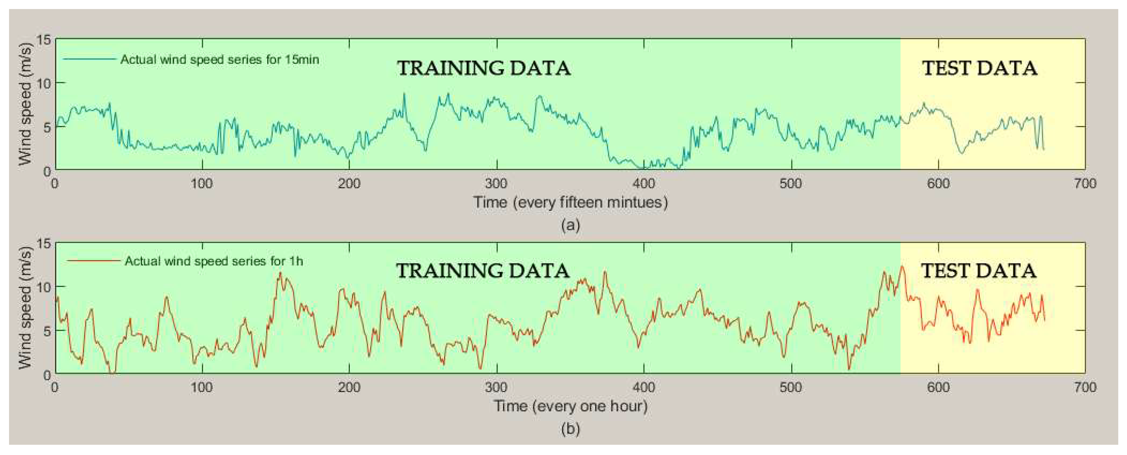
4.1. Study Area and Data Set
4.2. Performance Criteria of Prediction Accuracy
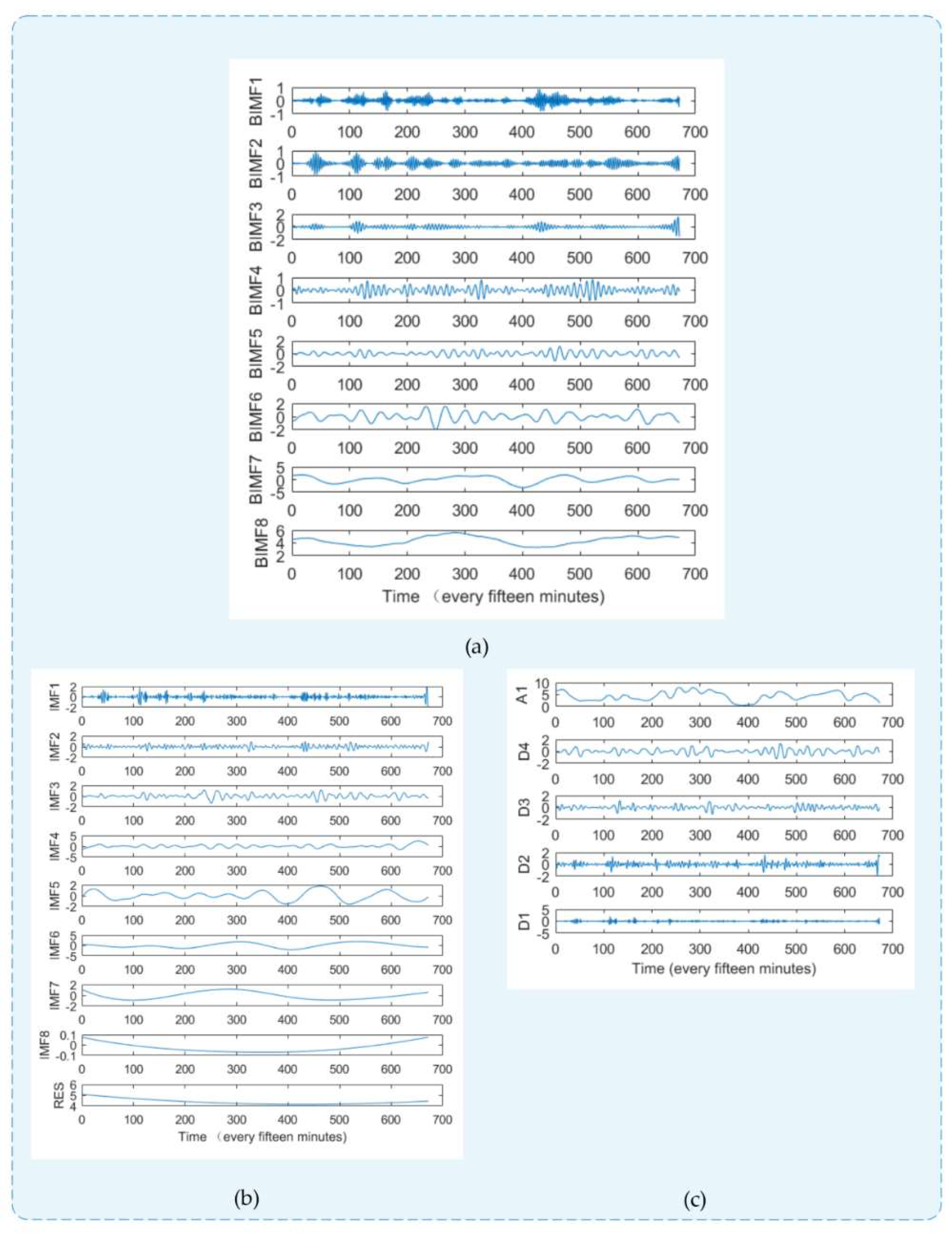
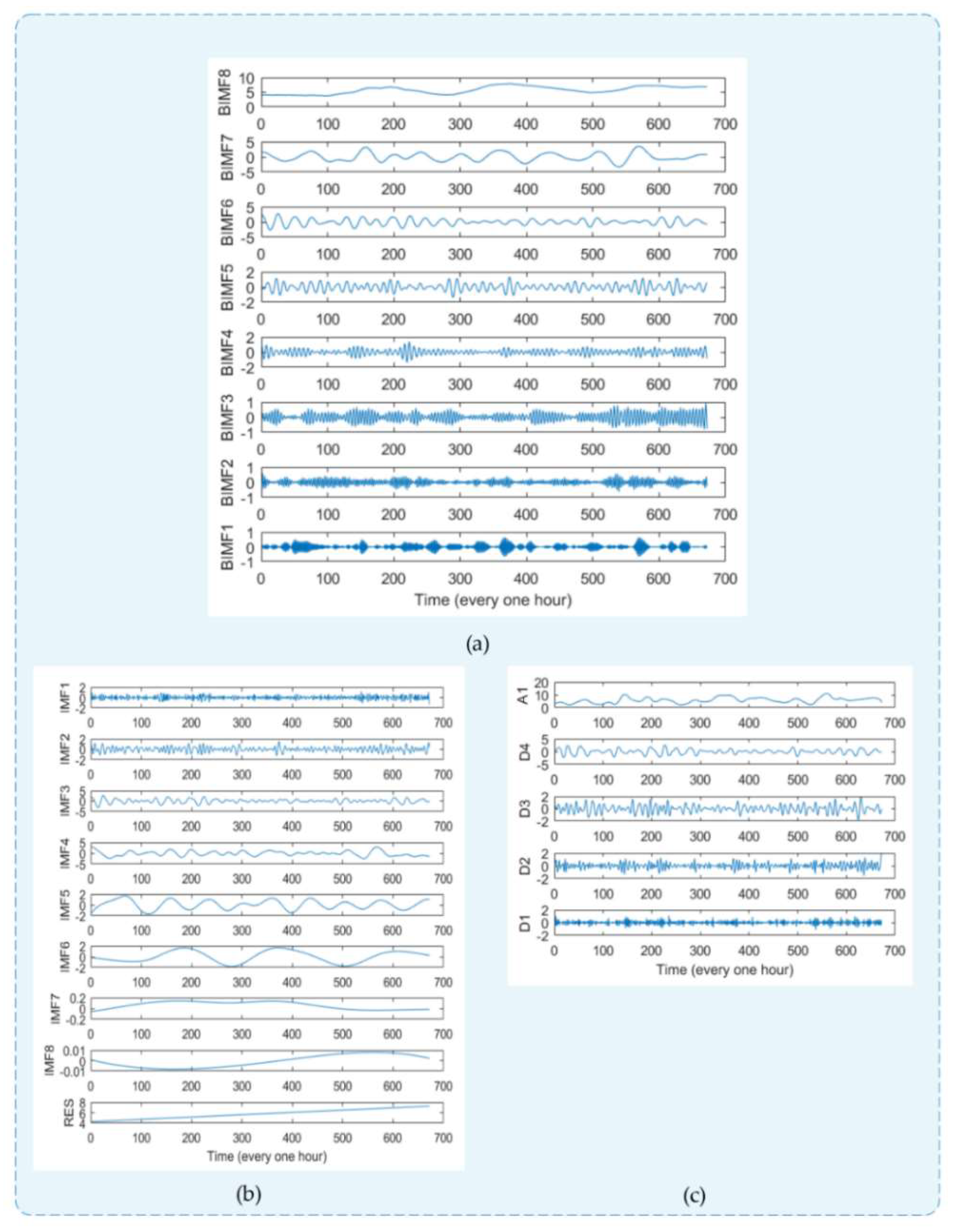
4.3. Original Wind Speed Series Decomposition Results
4.4. Parameter Settings
4.5. Comparative Analysis of Different Models
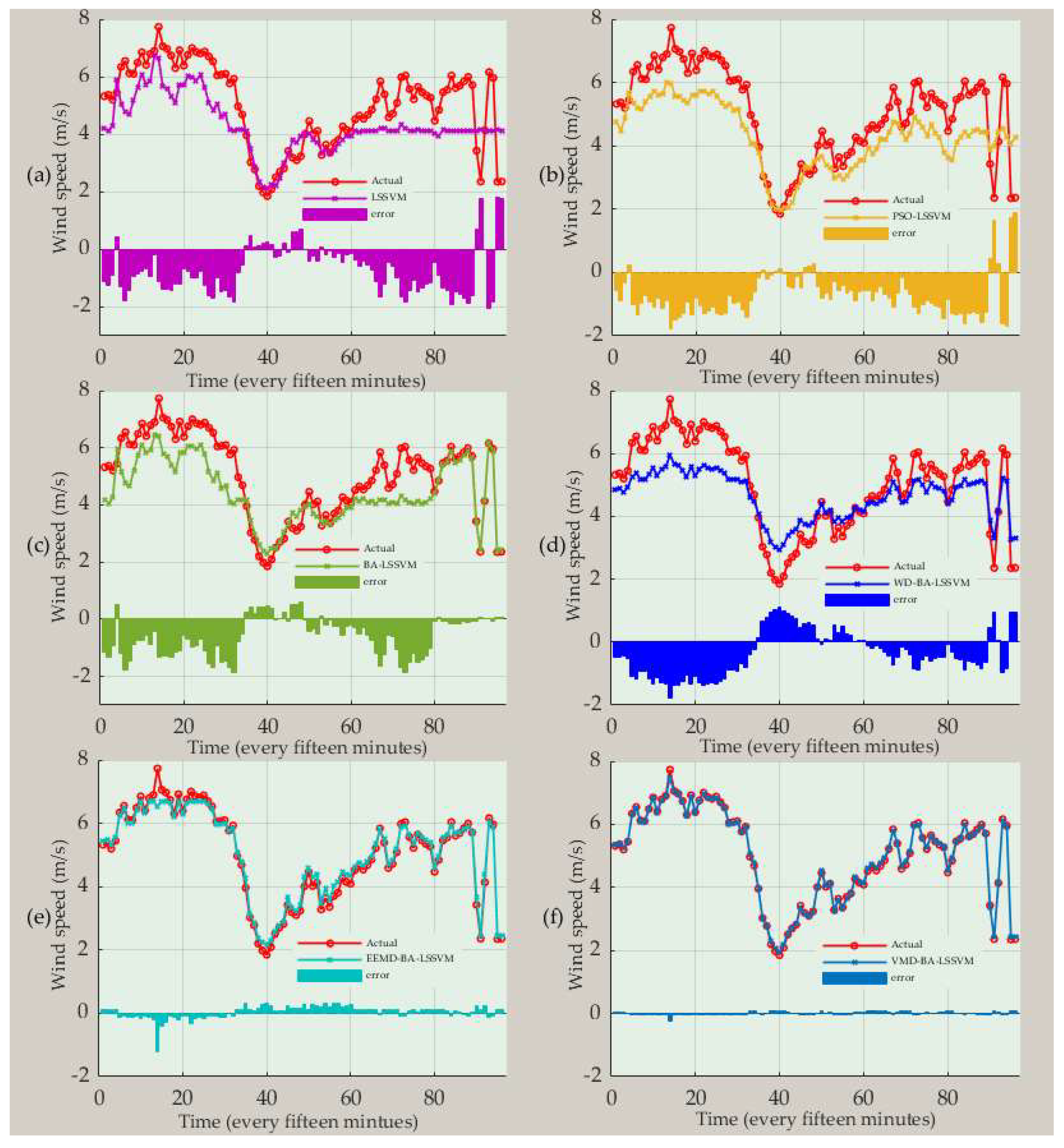
4.5.1. Case 1: Ultra Short-Term (15 min) Wind Speed Forecasting
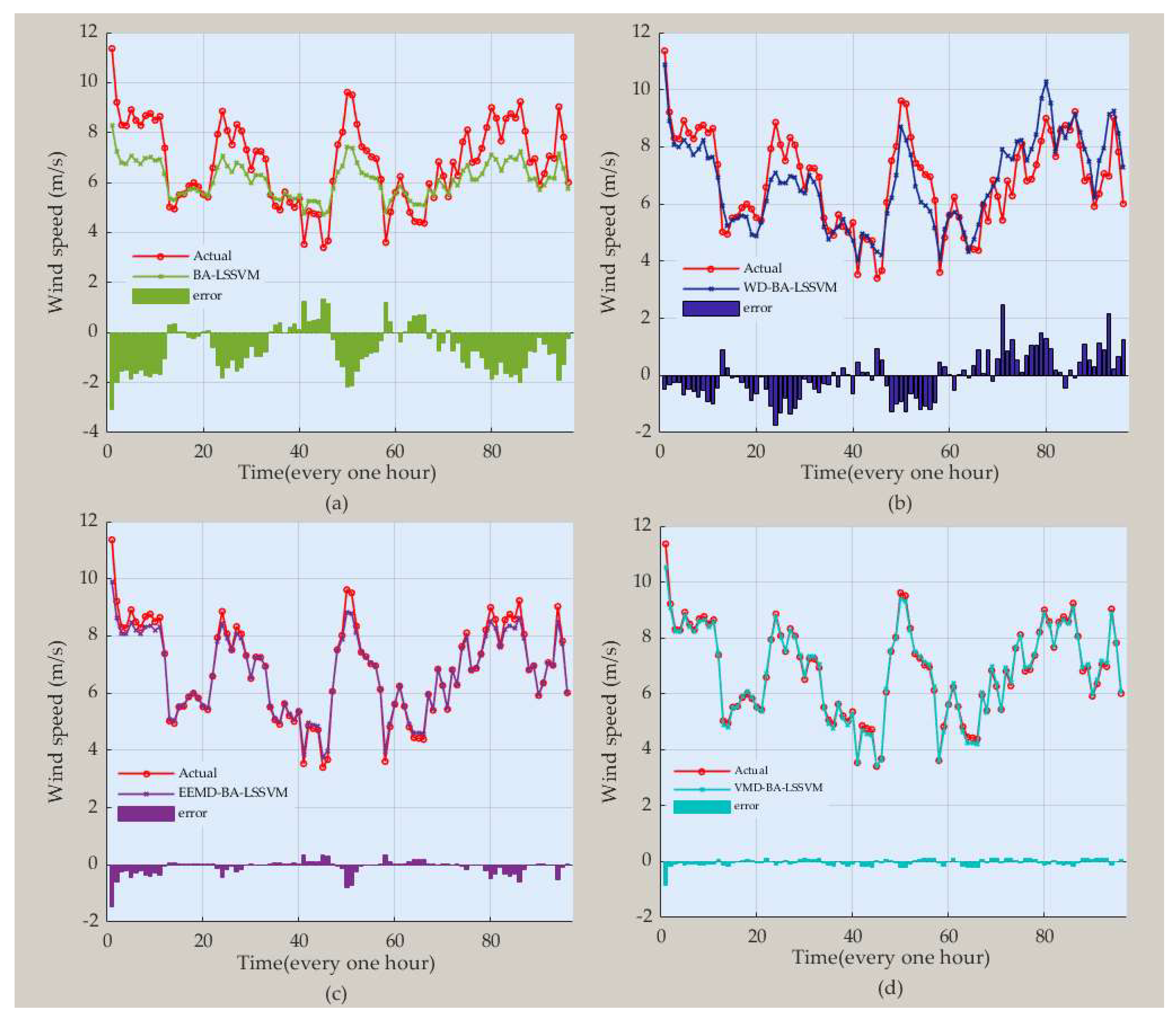
4.5.2. Case 2: Short-Term (1 h) Wind Speed Forecasting
5. Conclusions
Author Contributions
Acknowledgments
Conflicts of Interest
References
- Wu, Q.; Peng, C. Wind power generation forecasting using least squares support vector machine combined with ensemble empirical mode decomposition, principal component analysis and a bat algorithm. Energies 2016, 9, 261. [Google Scholar] [CrossRef]
- Kusiak, A.; Zhang, Z.J.; Verma, A. Prediction, operations, and condition monitoring in wind energy. Energy 2013, 60, 1–12. [Google Scholar] [CrossRef]
- Ackermann, T.; Söder, L. Wind energy technology and current status: A review. Renew. Sustain. Energy Rev. 2000, 4, 315–374. [Google Scholar] [CrossRef]
- Jung, J.; Broadwater, R.P. Current status and future advances for wind speed and power forecasting. Renew. Sustain. Energy Rev. 2014, 31, 762–777. [Google Scholar] [CrossRef]
- Barbounis, T.G.; Theocharis, J.B. A locally recurrent fuzzy neural network with application to the wind speed prediction using spatial correlation. Neurocomputing 2007, 70, 1525–1542. [Google Scholar] [CrossRef]
- Cassola, F.; Burlando, M. Wind speed and wind energy forecast through kalman filtering of numerical weather prediction model output. Appl. Energy 2012, 99, 154–166. [Google Scholar] [CrossRef]
- Erdem, E.; Shi, J. Arma based approaches for forecasting the tuple of wind speed and direction. Appl. Energy 2011, 88, 1405–1414. [Google Scholar] [CrossRef]
- Weron, R. Electricity price forecasting: A review of the state-of-the-art with a look into the future. Int. J. Forecast. 2014, 30, 1030–1081. [Google Scholar] [CrossRef]
- Maatallah, O.A.; Achuthan, A.; Janoyan, K.; Marzocca, P. Recursive wind speed forecasting based on hammerstein auto-regressive model. Appl. Energy 2015, 145, 191–197. [Google Scholar] [CrossRef]
- Liu, H.; Erdem, E.; Shi, J. Comprehensive evaluation of arma–garch(-m) approaches for modeling the mean and volatility of wind speed. Appl. Energy 2011, 88, 724–732. [Google Scholar] [CrossRef]
- Liu, H.; Tian, H.Q.; Chen, C.; Li, Y.F. A hybrid statistical method to predict wind speed and wind power. Renew. Energy 2010, 35, 1857–1861. [Google Scholar] [CrossRef]
- Liebl, D. Modeling and forecasting electricity spot prices: A functional data perspective. Ann. Appl. Stat. 2013, 7, 1562–1592. [Google Scholar] [CrossRef]
- Kani, S.A.P.; Riahy, G.H. A new ANN-based methodology for very short-term wind speed prediction using markov chain approach. In Proceedings of the IEEE Canada Electric Power Conference (EPEC 2008), Vancouver, BC, Canada, 6–7 October 2008; pp. 1–6. [Google Scholar]
- Wang, J.; Qin, S.; Zhou, Q.; Jiang, H. Medium-term wind speeds forecasting utilizing hybrid models for three different sites in xinjiang, china. Renew. Energy 2015, 76, 91–101. [Google Scholar] [CrossRef]
- Wei, S.; Liu, M. Wind speed forecasting using FEEMD echo state networks with RELM in Hebei, China. Energy Convers. Manag. 2016, 114, 197–208. [Google Scholar]
- Zhou, J.; Jing, S.; Gong, L. Fine tuning support vector machines for short-term wind speed forecasting. Energy Convers. Manag. 2011, 52, 1990–1998. [Google Scholar] [CrossRef]
- Yeh, W.C. New parameter-free simplified swarm optimization for artificial neural network training and its application in the prediction of time series. IEEE Trans. Neural Netw. Learn. Syst. 2013, 24, 661–665. [Google Scholar]
- Santamaria-Bonfil, G.; Reyes-Ballesteros, A.; Gershenson, C. Wind speed forecasting for wind farms: A method based on support vector regression. Renew. Energy 2016, 85, 790–809. [Google Scholar] [CrossRef]
- Gendeel, M.; Zhang, Y.X.; Han, A.Q. Performance comparison of ANNs model with VMD for short-term wind speed forecasting. IET Renew. Power Gener. 2018, 12, 1424–1430. [Google Scholar] [CrossRef]
- Zhang, W.; Qu, Z.; Zhang, K.; Mao, W.; Ma, Y.; Fan, X. A combined model based on ceemdan and modified flower pollination algorithm for wind speed forecasting. Energy Convers. Manag. 2017, 136, 439–451. [Google Scholar] [CrossRef]
- Amjady, N.; Keynia, F. Day ahead price forecasting of electricity markets by a mixed data model and hybrid forecast method. Int. J. Electr. Power Energy Syst. 2008, 30, 533–546. [Google Scholar] [CrossRef]
- Wang, J.Z.; Wang, Y.; Jiang, P. The study and application of a novel hybrid forecasting model—A case study of wind speed forecasting in china. Appl. Energy 2015, 143, 472–488. [Google Scholar] [CrossRef]
- Liu, T.X.; Liu, S.Z.; Heng, J.N.; Gao, Y.Y. A new hybrid approach for wind speed forecasting applying support vector machine with ensemble empirical mode decomposition and cuckoo search algorithm. Appl. Sci. l 2018, 8, 22. [Google Scholar] [CrossRef]
- Zahraee, S.M.; Assadi, M.K.; Saidur, R. Application of artificial intelligence methods for hybrid energy system optimization. Renew. Sustain. Energy Rev. 2016, 66, 617–630. [Google Scholar] [CrossRef]
- Liu, D.; Niu, D.; Wang, H.; Fan, L. Short-term wind speed forecasting using wavelet transform and support vector machines optimized by genetic algorithm. Renew. Energy 2014, 62, 592–597. [Google Scholar] [CrossRef]
- Wang, S.; Zhang, N.; Wu, L.; Wang, Y. Wind speed forecasting based on the hybrid ensemble empirical mode decomposition and ga-bp neural network method. Renew. Energy 2016, 94, 629–636. [Google Scholar] [CrossRef]
- Zhou, J.; Sun, N.; Jia, B.; Peng, T.; Sciubba, E. A novel decomposition-optimization model for short-term wind speed forecasting. Energies 2018, 11, 1752. [Google Scholar] [CrossRef]
- Liu, D.; Li, H.; Ma, Z. One hour ahead prediction of wind speed based on data mining. In Proceedings of the International Conference on Advanced Computer Control, Shenyang, China, 27–29 March 2010; pp. 199–203. [Google Scholar]
- Wang, D.Y.; Luo, H.Y.; Grunder, O.; Lin, Y.B.; Guo, H.X. Multi-step ahead electricity price forecasting using a hybrid model based on two-layer decomposition technique and bp neural network optimized by firefly algorithm. Appl. Energy 2017, 190, 390–407. [Google Scholar] [CrossRef]
- Zosso, D.; Dragomiretskiy, K. Variational mode decomposition. IEEE Trans. Signal Process. 2014, 62, 531–544. [Google Scholar]
- Wang, Y.; Markert, R.; Xiang, J.; Zheng, W. Research on variational mode decomposition and its application in detecting rub-impact fault of the rotor system. Mech. Syst. Signal Process. 2015, 60–61, 243–251. [Google Scholar] [CrossRef]
- Huang, N.E.; Shen, Z.; Long, S.R.; Wu, M.C.; Shih, H.H.; Zheng, Q.; Yen, N.-C.; Tung, C.C.; Liu, H.H. The empirical mode decomposition and the hilbert spectrum for nonlinear and non-stationary time series analysis. Proc. R. Soc. Lond. Ser. A Math. Phys. Eng. Sci. 1998, 454, 903–995. [Google Scholar] [CrossRef]
- Mallat, S.G. A theory for multiresolution signal decomposition: The wavelet representation. IEEE Trans. Pattern Anal. Mach. Intell. 1989, 11, 674–693. [Google Scholar] [CrossRef]
- Suykens, J.A.K.; Vandewalle, J. Recurrent least squares support vector machines. IEEE Trans. Circuits Syst. I Fundam. Theory Appl. 2008, 47, 1109–1114. [Google Scholar] [CrossRef]
- Cheng, L.I. A new metaheuristic bat-inspired algorithm. Comput. Knowl. Technol. 2010, 284, 65–74. [Google Scholar]


| Variable | Meaning | Variable | Meaning |
|---|---|---|---|
| real-valued signal | center pulsation | ||
| band-limited intrinsic mode function | Lagrangian multipliers |
| Variable | Meaning | Variable | Meaning |
|---|---|---|---|
| raw signal | residue | ||
| intrinsic mode function | random white Gaussian noise series |
| Variable | Meaning | Variable | Meaning |
|---|---|---|---|
| raw signal | approximate sequence | ||
| detail sequence |
| Variable | Meaning | Variable | Meaning |
|---|---|---|---|
| prediction value | Error | ||
| Input | Lagrange multipliers | ||
| Output | complex degree | ||
| regularization parameter | parameter of the kernel function |
| Case | Data Set | Statistics | ||||
|---|---|---|---|---|---|---|
| Minimum (m/s) | Maximum (m/s) | Mean (m/s) | Median (m/s) | Standard Deviation (m/s) | ||
| 15 min | Training data | 0.11 | 8.8 | 4.278 | 4.35 | 1.978 |
| Test data | 1.85 | 7.73 | 5.016 | 5.335 | 1.455 | |
| 1 h | Training data | 0 | 12.31 | 5.594 | 5.476 | 2.5 |
| Test data | 3.4 | 11.36 | 6.81 | 6.902 | 1.617 |
| Parameters | Values | Parameters | Values |
|---|---|---|---|
| Initial population size | 10 | Minimum frequency | 0 |
| Initial loudness | 0.25 | Maximum frequency | 5 |
| Pulse rate | 0.5 | Max-iteration number | 50 |
| VMD | EEMD | WD | ||||||
|---|---|---|---|---|---|---|---|---|
| Components | Components | Components | ||||||
| BIMF1 | 0.1898 | 14.8432 | IMF1 | 0.098 | 9.5004 | A1 | 0.1696 | 10.1624 |
| BIMF2 | 12.3084 | 1.0987 | IMF2 | 0.2118 | 0.0239 | D1 | 0.0014 | 8.1789 |
| BIMF3 | 1.3475 | 0.4603 | IMF3 | 0.2942 | 0.0532 | D2 | 13.6794 | 10.1307 |
| BIMF4 | 5.6934 | 2.2004 | IMF4 | 24.51 | 2.4311 | D3 | 4.5363 | 0.4641 |
| BIMF5 | 8.4486 | 4.7532 | IMF5 | 1983.8 | 0.1635 | D4 | 0.0092 | 11.1173 |
| BIMF6 | 0.811 | 6.835 | IMF6 | 28.3727 | 0.303 | |||
| BIMF7 | 9.1664 | 0.8689 | IMF7 | 80.9834 | 0.3148 | |||
| BIMF8 | 8.8698 | 9.4069 | IMF8 | 3.87 | 0.5182 | |||
| RES | 0.728 | 0.0892 | ||||||
| Case 1 | Error | Model | |||||
| LSSVM | PSO-LSSVM | BA-LSSVM | WD-BA-LSSVM | EEMD-BA-LSSVM | VMD-BA-LSSVM | ||
| Fifteen Minutes | MAPE | 20.99% | 19.69% | 15.44% | 14.93% | 3.42% | 1.03% |
| MAE | 0.92 | 0.8708 | 0.6873 | 0.6972 | 0.1538 | 0.0427 | |
| RMSE | 1.0866 | 0.9858 | 0.8764 | 0.8094 | 0.2035 | 0.0543 |
| Case 2 | Error | Model | |||
| BA-LSSVM | WD-BA-LSSVM | EEMD-BA-LSSVM | VMD-BA-LSSVM | ||
| One hour | MAPE | 14.42% | 9.50% | 2.23% | 1.56% |
| MAE | 0.9283 | 0.6463 | 0.1585 | 0.1015 | |
| RMSE | 1.1309 | 0.8026 | 0.2715 | 0.1367 | |
© 2019 by the authors. Licensee MDPI, Basel, Switzerland. This article is an open access article distributed under the terms and conditions of the Creative Commons Attribution (CC BY) license (http://creativecommons.org/licenses/by/4.0/).
Share and Cite
Wu, Q.; Lin, H. Short-Term Wind Speed Forecasting Based on Hybrid Variational Mode Decomposition and Least Squares Support Vector Machine Optimized by Bat Algorithm Model. Sustainability 2019, 11, 652. https://doi.org/10.3390/su11030652
Wu Q, Lin H. Short-Term Wind Speed Forecasting Based on Hybrid Variational Mode Decomposition and Least Squares Support Vector Machine Optimized by Bat Algorithm Model. Sustainability. 2019; 11(3):652. https://doi.org/10.3390/su11030652
Chicago/Turabian StyleWu, Qunli, and Huaxing Lin. 2019. "Short-Term Wind Speed Forecasting Based on Hybrid Variational Mode Decomposition and Least Squares Support Vector Machine Optimized by Bat Algorithm Model" Sustainability 11, no. 3: 652. https://doi.org/10.3390/su11030652
APA StyleWu, Q., & Lin, H. (2019). Short-Term Wind Speed Forecasting Based on Hybrid Variational Mode Decomposition and Least Squares Support Vector Machine Optimized by Bat Algorithm Model. Sustainability, 11(3), 652. https://doi.org/10.3390/su11030652