The Impact of Land Use/Land Cover Change (LULCC) on Water Resources in a Tropical Catchment in Tanzania under Different Climate Change Scenarios

Abstract

Many parts of sub-Saharan Africa (SSA) are prone to land use and land cover change (LULCC). In many cases, natural systems are converted into agricultural land to feed the growing population. However, despite climate change being a major focus nowadays, the impacts of these conversions on water resources, which are essential for agricultural production, is still often neglected, jeopardizing the sustainability of the socio-ecological system. This study investigates historic land use/land cover (LULC) patterns as well as potential future LULCC and its effect on water quantities in a complex tropical catchment in Tanzania. It then compares the results using two climate change scenarios. The Land Change Modeler (LCM) is used to analyze and to project LULC patterns until 2030 and the Soil and Water Assessment Tool (SWAT) is utilized to simulate the water balance under various LULC conditions. Results show decreasing low flows by 6–8% for the LULC scenarios, whereas high flows increase by up to 84% for the combined LULC and climate change scenarios. The effect of climate change is stronger compared to the effect of LULCC, but also contains higher uncertainties. The effects of LULCC are more distinct, although crop specific effects show diverging effects on water balance components. This study develops a methodology for quantifying the impact of land use and climate change and therefore contributes to the sustainable management of the investigated catchment, as it shows the impact of environmental change on hydrological extremes (low flow and floods) and determines hot spots, which are critical for environmental development.

1. Introduction

Recent developments in sub-Saharan Africa (SSA) show an increasing trend of conversion of natural land cover into arable land [1,2,3,4,5,6,7,8,9,10,11]. Drivers of change are manifold and can be directly linked to human activities such as population growth, economic development, and globalization [11,12]. Natural processes like floods, landslides, droughts and climate change affect land use and land cover change (LULCC) [9], although they are induced by anthropogenic activities to a certain degree. These conversions into arable land have an adverse impact on several ecosystem services as a trade-off for increased agricultural outputs such as food and timber production [9,13]. Several water-related targets of the Sustainable Development Goals (SDGs) are at risk due to land conversions into arable land, especially with regard to SDG 6 (Clean Water and Sanitation) and SDG 15 (Life on Land) [13,14].

Several studies investigated the impact of LULCC and climate change on water resources separately [3,15] or simultaneously [16,17]. The results of the studies differ due to several reasons e.g., the type of LULCC, the regional focus, or the time period and model chosen to simulate climate change. However, many studies indicate an increased exposure to hydro-climatic extremes in Eastern Africa [18,19,20,21]. This study exemplarily analyzes LULCC compared to climate change in the Kilombero Catchment in Tanzania and how these affect water resources. The catchment itself is subject to aforementioned LULCC [1,13] and pressure on land resources in the valley is fostered by government plans to implement the Southern Agricultural Growth Corridor of Tanzania (SAGCOT) [22], which is accompanied by a growing population and migration of pastoralists into the valley [23]. SAGCOT follows a green growth approach covering three development clusters in Kilombero, Ihemi, and Mbarali, comprising one third of the mainland of Tanzania [1,24,25]. On the one hand the key clusters are characterized by great agricultural potential and on the other hand they contain extensive forests, protected areas, and their infrastructure is poorly developed [1]. One of the key features of the SAGCOT initiative for the Kilombero cluster is the establishment of a sustainable agricultural intensification with irrigation schemes for rice and sugarcane as well as integrated crop-livestock-aquaculture systems in the catchment’s wetland [24]. These changes in LULC in combination with the effects of climate change complicate water resource management of the catchment. Yet, projections concerning water quantities are crucial to sustaining the socio-ecological system and long-term perspectives are especially essential for a responsible treatment of water resources under changing climatic conditions.

The dominant LULCC in the catchment is from grassland to cropland, which mainly occurs in its floodplain area [1,26]. The most important crop for this conversion is rain-fed rice, that is grown in the lowland areas [13,27]. However, deforestation is becoming more important with the increasing population and the growing demand for timber, fuelwood and charcoal production [28]. Other drivers of change are economic development, foreign agricultural investments, agro-technological advancements, favorable biophysical factors, policies, the aforementioned population growth, and increased migration of pastoralists into the valley [23,28]. These LULCC will affect ecosystem services and water resources in the catchment and scientific guidance is needed in order to enable a sustainable development of the catchment [1,13]. Inhabitants of the catchment already report changing water dynamics, such as lower water levels and consequently depleted fish stocks [28]. Paddy rice plays a specific role in this study due to its large-scale suitability in the catchment according to the SAGCOT plans [22] and additionally due to its high water demand and the resulting implications on water resources [29]. The following goals of the study arose from this context:

(i)

Develop scenarios for the LULC distribution for the Kilombero Catchment until 2030;

(ii)

Analyze the impact of the different LULC scenarios on water resources at various temporal and spatial scales;

(iii)

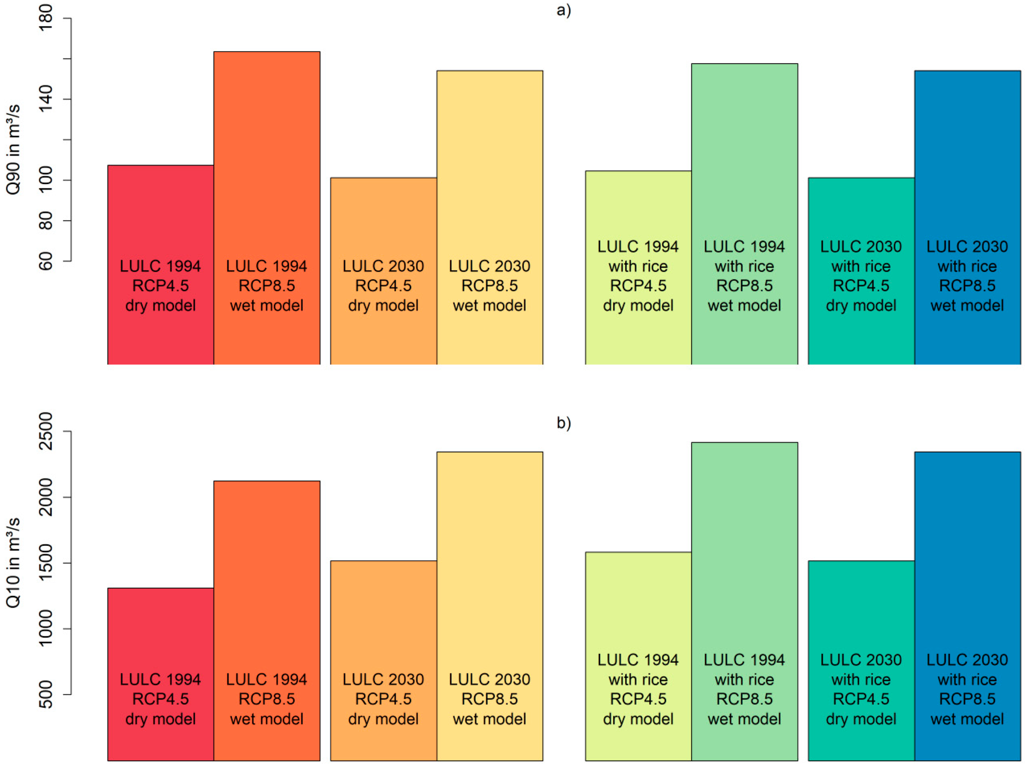
Investigate the impact of LULCC on low flow and high flow regimes;

(iv)

Assess the combined impact of LULCC and climate change on water resources.

In order to reach these goals, observed patterns of change were correlated with various spatial features of the catchment using the digital elevation model (DEM), and were projected until 2030 by using the Land Change Modeler (LCM) [30,31,32]. Furthermore, the SWAT model was utilized to simulate the impact of the different LULC setups on water resources. Subsequently, the selected Global Climate Model-Regional Climate Model (GCM-RCM) developed for a previous study [33] was integrated to estimate the combined effect of LULCC and climate change. Results show huge deviations in water balance components on a subcatchment scale and that especially high flow patterns vary among the different LULC scenarios.

An overview of abbreviations that are used within this study and their meanings is given in

Table 1. List of abbreviations used in this study and their meanings.

Abbreviation	Meaning	Abbreviation	Meaning
CLMcom	Climate Limited-area Modeling Community	Q10	Flow exceeded in 10% of the specified period
CORDEX	Coordinated Regional Downscaling Experiment	Q90	Flow exceeded in 90% of the specified period
DEM	Digital elevation model	RCM	Regional climate models
EPIC	Erosion-Productivity Impact Calculator	RCP	Representative Concentration Pathways
GCM	Global Climate Model	RF	Random Forest
HRU	Hydrologic response unit	RBWB	Rufiji Basin Water Board
HWSD	Harmonized World Soil Database	SAGCOT	Southern Agricultural Growth Corridor of Tanzania
KGE	Kling-Gupta efficiency	SCS	Soil conservation service
LCM	Land Change Modeler	SDGs	Sustainable Development Goals
LULC	Land use/land cover	SMHI	Swedish Meteorological and Hydrological Institute
LULCC	Land use/land cover change	SRTM	Shuttle Radar Topography Mission
MLP	Multi-Layer Perceptron	SSA	Sub-Saharan Africa
MSS	Multispectral scanner	SWAT	Soil and Water Assessment Tool
NGO	Non-Governmental Organisation	TMA	Tanzania Meteorological Agency
NSE	Nash-Sutcliffe-Efficiency	UDSM	University of Dar es Salaam
PPP	Public-private partnership

.

2. Materials and Methods

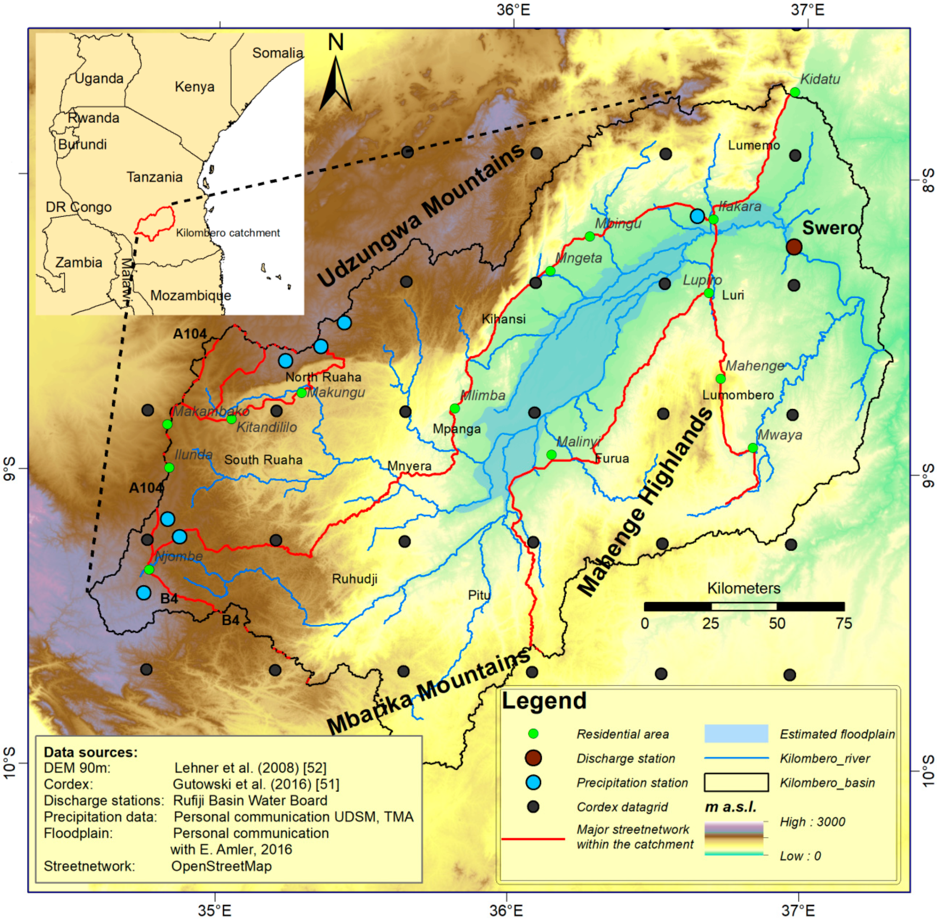
2.1. Study Site

The study site is located in the Morogoro region in south central Tanzania (Figure 1). It is enclosed by the Udzungwa Mountains in the north and west, whereas the Mbarika Mountains and the Mahenge Highlands demarcate the southern boundary of the catchment. The catchment is drained by the eponymous Kilombero River and comprises a total of 40,240 km² up to the confluence of the Kilombero River and the Luwego River [2]. From here downstream, the river is called Rufiji River and refers to the Rufiji Basin, which is the most important river basin of Tanzania [34]. The Rufiji Basin consists of three major tributaries and their respective catchments, which are the Great Ruaha, the Luwego, and the Kilombero. The Kilombero itself covers only 23% of the Rufiji Basin´s area, but it contributes 62% of total discharge and is therefore of particular importance with regard to water resources [35]. The Kilombero River itself has several perennial and seasonal tributaries, which mainly contribute inflow from the upland areas. However, this system is at risk, due to LULCC and water abstractions that affect the inflow of several tributaries and the maintenance of the environmental flows [34,36]. The Kilombero river forms a complex braided and meandering river network in the central floodplain, which covers 7967 km² and constitutes one of the most important African lowland fresh water wetlands [35,37]. Since 2002 the floodplain has been designated as a Ramsar site and over 70% of the floodplain area is protected [38].

The climate is a sub-humid tropical climate with a distinctive seasonality, which is characterized by a dry and a rainy season. The rainy season itself can be differentiated into the short rainy season from October until December/January (locally called “Masika”) and the long rainy season from March until May (“Vuli”) [39,40]. Nevertheless, this bimodal pattern only applies for the northern parts of Tanzania, whereas the south-western parts of Tanzania are characterized by a unimodal rainfall distribution and therefore one rainy season (“Msimu”) [41]. However, there are huge interannual, intraannual, and also spatial variabilities in the distribution of precipitation for the Kilombero Catchment recorded [2,33,42]. This high variability can be attributed to the manifold factors influencing the local climate, such as remote forcings (e.g., Walker Circulation, Indian Ocean Dipole), regional circulations (e.g., Tropical Easterly Jet), but also local geographic factors (e.g., windward and leeward effects) [43]. Annual mean areal precipitation is between 1200 and 1400 mm, whereas the mountainous parts receive up to 2100 mm and the valley 1100 mm, respectively [35,42]. The mean annual temperature has an antagonistic pattern and varies between 24 °C in the valley and around 17 °C in the uplands of the catchment [35].

Soils in the floodplain are largely heavy black cotton soils, with a good water content at field capacity, but also some patches of sandy soils [23]. According to the Harmonized World Soil Database (HWSD) most parts of the catchment are covered by acrisols, with some areas dominated by cambisols in the western part and nitisols in the Udzungwa mountains [44].

The land cover of the upper catchment embraces a mixture of natural vegetation like tropical rainforests, bush lands, and wooded grasslands with some patches of agricultural fields [45]. The valley is surrounded by a miombo woodland belt with mainly Brachystegia spp., whereas the floodplain itself is dominated by agricultural use and tall grasses such as Penisetum purpureum, Panicum maximum, Hyparrhenia spp., and Phragmites mauritianus with some isolated trees of Ficus spp. and Kigelia africana [38,46]. The most important crops grown in the valley are sugarcane (Saccharum officinarum), maize (Zea mays), paddy rice (Oryza sativa), and cassava (Manihot esculata) [23]. Rice production is dominated by small-scale farmers and rain-fed agriculture, although some small irrigations schemes do exist in the valley. Sugarcane is mainly grown as irrigated agriculture by a large-scale contractor (Kilombero Sugar Company) in the northeastern part of the catchment.

Recent developments show an increasing trend of conversion of wetland, forested areas, and grassland into arable land in the Kilombero Valley [1,2]. The Kilombero area has to cope with many immigrants, including a high number of pastoralists, causing a population growth rate for the Kilombero area of 3.4% according to the national population census from 2012, which exceeded the national average of 2.8% [47]. The SAGCOT growth corridor plans, including infrastructure developments like bridge construction and expansion of paved roads [22,24], as well as the planning of the Stiegler´s Gorge hydropower dam in the Selous Game Reserve downstream, might have a huge impact on the development of the catchment [34].

2.2. Input Data

The SWAT model for this study is based on the details already given by Näschen et al. [2]. The issue of data scarcity in the study region is solved by using freely available geodata in combination with data gathered from local partners in Tanzania (

Table 2. Overview of the applied datasets, their resolution, sources, and the required parameters in this study.

Data Set	Resolution/Scale	Source	Required Parameters
Digital elevation model (DEM)	90 m	Shuttle Radar Topography Mission (SRTM) [52]	Topographical data
Soil map	1 km	FAO [44]	Soil classes and physical properties
Land use map	60 m (1970s), 30 m (1994, 2004, 2014)	Landsat Pre-Collection Level-1 [53], Landsat TM, ETM+, OLI Surface Reflectance Level-2 Science Products [54,55], SRTM [52]	Land use/cover classes
Precipitation	Daily	Personal communication: Rufiji Basin Water Board (RBWB), University of Dar es Salaam (UDSM), Tanzania Meteorological Agency (TMA)	Measured precipitation
Climate	Daily/0.44° (1951–2060)	CORDEX Africa [51]	Temperature, humidity, solar radiation, wind speed, precipitation
Discharge	Daily (1958–1970)	RBWB [48]	Discharge

, [48]). The most crucial but also most limiting data is discharge data, which has the longest time series at a downstream station (“Swero”) near the outlet of the catchment but stretches in good quality only from 1958 to 1970. The station is currently being renewed and new stations are being set up in the catchment, nonetheless there is no time series and no rating curve for the new stations available up to today. Therefore, the historical discharge data was used to set up the hydrological model [2]. In addition, LULC maps were produced from Landsat imagery for four different time steps. Due to extensive cloud cover, all available Landsat TM, ETM+, and OLI Surface Reflectance scenes within three-year periods around the years 1994, 2004, and 2014 were considered, and multi-temporal metrics [49] were calculated using different vegetation indices. Together with topographic indices based on the Shuttle Radar Topography Mission (SRTM) DEM, these were classified in a supervised Random Forest (RF) approach [2,50]. The RF classifier was calibrated and validated using information from field visits, flight campaigns and Google Earth in a random sampling scheme. For the 1970s LULC map, due to the lack of suitable images, Landsat pre-Collection Level 1 images from the whole decade were cloud-masked, corrected for corrupted image lines, normalized to one master image, mosaicked, and classified. The spatial resolution of the early Landsat images (1970s) from the multispectral scanner (MSS) instrument is 60 m. The resulting maps were resampled to a 30 m pixel size in order to be complementary to the other Landsat products. Figure 2 shows the LULC maps as reclassified into SWAT LULC classes. The left configurations (a–d) include a barren class and an undifferentiated cropland class, whereas the right configurations (e–h) differentiate between cropland and rice as a specific plant (named “cropland-rice”). SWAT classes besides barren, cropland, and cropland-rice comprise forest evergreen, forest mixed, grassland, savanna, wetland, open water, and built-up.

Seven precipitation stations were used as input in combination with Coordinated Regional Downscaling Experiment (CORDEX) Africa data [51] for the other climate parameters (Table 2). For future climate scenarios GCM-RCM (Global Climate Models-Regional Climate Models) model combinations from CORDEX Africa were bias-corrected for temperature and precipitation. A more detailed description on the procedure can be found in Näschen et al. 2019 [33]. Two of these GCM-RCM scenario data sets were chosen for this study in order to represent a span of wet and dry scenarios covering increasing and decreasing annual precipitation amounts (

Table 3. Overview of the Regional Climate Models (RCMs), their driving Global Climate Models (GCMs), and the assigned naming for the model combination within this study.

GCM	RCM	Institution	URL	In This Study Referred to as
CNRM-CM5	CCLM4-8-17_v1	Climate Limited-area Modeling Community (CLMcom)	https://esg-dn1.nsc.liu.se/	Dry model
MIROC5	RCA4_v1	Rossby Centre, Swedish Meteorological and Hydrological Institute (SMHI)	https://esg-dn1.nsc.liu.se/	Wet model

,

Table 4. Historical annual average precipitation according to the bias-corrected RCM simulations (1951–2005) and the absolute and relative changes of precipitation, actual evapotranspiration and overall water yield in SWAT simulations (2010–2060) according to the projections based on RCP4.5 and RCP8.5 scenarios. Numbers in parentheses represent the changes in percentage (modified based on reference [33]).

Climate Model	Historical Precipitation (after Bias Correction) in mm	RCP Precipitation Changes in mm (%)	RCP Actual Evapotranspiration Changes in mm (%)	RCP Overall Water Yield Changes in mm (%)
“Dry Model” (RCP4.5)	1311	−109 (−8.3)	−10 (−1.4)	−103 (−19.8)
“Wet Model” (RCP4.5)	1345	218 (16.2)	14 (1.5)	163 (42.1)
“Dry Model” (RCP8.5)	1311	−76 (−5.8)	11 (1.5)	−85 (−16.3)
“Wet Model” (RCP8.5)	1345	302 (22.5)	25 (2.7)	239 (61.6)

). Soil data was gathered from the Harmonized World Soil Database (HWSD) and the SRTM 90 m digital elevation model (DEM) was used for the SWAT model. A complete overview on all of the data sources utilized in this study is given in Table 2.

2.3. Modeling Approach

2.3.1. The SWAT Model

In this study the SWAT model [56] was applied to simulate the hydrological processes on the catchment scale. SWAT is a semi-distributed and physically-based model which operates on a daily time-scale. The physically-based approach of SWAT with the incorporation of the Erosion-Productivity Impact Calculator (EPIC) model [57] allows to account for plant growth variations and is necessary to adequately simulate the impacts of land use changes on hydrological processes.

In a first step the SWAT model discretizes the catchment into subcatchments based on a threshold that defines the minimum drainage area to form a stream. Furthermore, these subcatchments are discretized into hydrologic response units (HRU), which are unique combinations of soil, slope, and land use within each of the subcatchments. These HRUs are the most important spatial unit for the calculation of hydrological processes within SWAT.

In general, the model differentiates between a land phase and a routing phase. The land phase considers most of the hydrological processes of the hydrological cycle, whereas the routing phase integrates the routing of water among the subcatchments and in-stream processes of water, sediments, nutrients, and organic chemicals. In the land phase the water balance equation is solved on HRU level and all HRU calculations are treated as the result of a subcatchment without considering routing among the single HRUs. Climate data input is given on the subcatchment scale, with the option to account for altitudinal effects on temperature or precipitation with so called elevation bands. These elevation bands modify temperature and precipitation to represent orographic effects in case of large altitudinal differences within the subcatchments [58]. Precipitation can be intercepted by vegetation, enter the reach directly or hit the ground, where it might move as surface runoff, evaporate, or infiltrate into the soil based on the given physical conditions represented by the Soil Conservation Service (SCS) curve number and the climatic conditions [59,60]. Once water infiltrates into the soil, it is stored as soil moisture and can move among up to ten soil layers using a storage routing technique, which is based on the field capacity of the soil layers and the saturated hydraulic conductivity. Lateral flows in the soil are simulated with a kinematic storage model, which mainly depends on the slope of the area [61]. Groundwater is divided into two aquifers in SWAT: A shallow unconfined aquifer and a deeper confined aquifer. If water percolates from the soil through the unsaturated zone, it enters the shallow aquifer. From there, water might contribute as baseflow to the reach, move upwards as capillary rise due to LULC dependent water demand, or percolate deeper into the confined aquifer, where it is assumed to contribute to the regional water balance and is treated as being lost for the local catchment. However, both aquifers might contribute to the streamflow through different parameters [62]. A detailed model description is given by Arnold et al. [56], Neitsch et al. [58], and Arnold et al. [63].

2.3.2. Model Setup, Evaluation and Extreme Value Analysis (SWAT Model)

The SWAT model setup was done with ArcSWAT 2012 (revision664), whereas calibration and validation were performed with SWAT-CUP (version 5.1.6.2) and the SUFI-2 algorithm [64] using the Kling-Gupta efficiency (KGE) as an objective function. The catchment was divided into 95 subcatchments and 1087 HRUs. Additionally elevation bands were integrated to adequately account for varying precipitation patterns due to high relief energy within the subcatchments [2,58]. The coefficient of determination (R²) (Equation (1)), the Nash-Sutcliffe-Efficiency (NSE) (Equation (2)), and the aforementioned KGE (Equation (3)) were some of the utilized evaluation criteria. A more detailed overview on the SWAT model setup and additional evaluation criteria is given by Näschen et al. [2].

$$R^2=\frac{{\left[{{\displaystyle \sum }}_{i=1}^n\left(O_i-\overline{O}\right)\left(S_i-\overline{S}\right)\right]}^2}{{{\displaystyle \sum }}_{i=1}^n{\left(O_i-\overline{O}\right)}^2{{\displaystyle \sum }}_{i=1}^n{\left(S_i-\overline{S}\right)}^2}$$

(1)

$$NSE=1-\frac{{{\displaystyle \sum }}_{i=1}^n{\left(O_i-S_i\right)}^2}{{{\displaystyle \sum }}_{i=1}^N{\left(O_i-\overline{O}\right)}^2}$$

(2)

$$KGE=1-\sqrt{{\left(r-1\right)}^2+{\left(\sigma -1\right)}^2+{\left(\beta -1\right)}^2}$$

(3)

where n is the number of observations, $O_i$ and $S_i$ are the observed and simulated discharge values, respectively, and $\overline{O}$ and $\overline{S}$ are the mean of observed and simulated discharge values. r is the coefficient of correlation between observed and simulated data, $\sigma$ is the ratio of the standard deviation of simulated and observed data, and β is the ratio of the means of simulated and observed data.

The results of the SWAT model were utilized to analyze changes in low flows and high flows for the different LULC setups separately and in combination with selected RCM-GCMs (Table 3). The extRemes 2.0 package [65] was utilized to calculate return levels from 2-year up to 100-year return levels using the generalized extreme value distributions (GEV) (Equations (4) and (5)) and the generalized maximum likelihood estimation (GMLE) method:

$$F(x)=exp[-{\{1+\gamma (\frac{x-\mu }{\alpha }\left)\right\}}^{-1/\mu }]$$

(4)

where $\gamma$ is the shape parameter, $\mu$ the location parameter, and $\alpha$ the scale parameter of the probability distribution function with $\alpha >0$ and ($1+\gamma \left(x-\mu \right)/\alpha$) $>0$. If $\gamma \to 0$, the function belongs to the Gumbel family and is as follows:

$$F\left(x\right)=\exp \left[-\exp \left\{-\left(\frac{x-\mu }{\alpha }\right)\right\}\right].$$

(5)

Additionally, the Q10 index was applied, because it is less sensitive to outliers compared to the generalized extreme value analysis. The Q10 is defined as the daily discharge that is exceeded in 10% of all the simulations here. Moreover, the Q90 [66,67] index was used to analyze low flows. In contrast to the Q10 index, the Q90 index is defined as daily discharge that is exceeded in 90% of all the simulations here. The Hydrostats package [68] in the statistical software R was applied for these analyses.

2.3.3. Land Use and Land Cover Change (LULCC) Scenarios

One of the main objectives of this article is to analyze the impact of LULCC on water resources until 2030. Therefore, scenarios of LULC for 2030 were developed using a mixed method approach containing land use change modeling, expert interviews, and a participatory mapping exercise in the framework of a workshop with local experts (Figure 3). The main goal of developing the 2030 scenarios was to identify implications of potential future LULC distributions on water resources in order to determine hot spots of change regarding water resources. In a first step, the historical LULC distributions from the 1970s until 2014 were derived from Landsat images (see Section 2.2). The Land Change Modeler LCM [31,32,69,70], within the Terrset Software Version 18.31 utilizing the IDRISI GIS System [32], was used to analyze the changes of LULC classes among the available historical products from the 1970s until 2014 (“Analysis of Change”, Figure 3).

The next step consisted of a mixture of quantitative and qualitative methods to estimate potential drivers of change. The quantitative part analyzed the changes of all LULC classes between two time steps and finally identified potential explanatory factors for change. This was achieved by utilizing the evidence likelihood transformation integrated in the LCM to identify explanatory factors based on observed changes among the maps of 2004 and 2014. These time steps were identified as most suitable baseline for project changes for the period until 2030, because changes from the 1970s until 2004 are rather negligible (Figure 2). This procedure was done separately for the LULC maps covering cropland only, as well as for the maps that distinguish between cropland and cropland-rice (Figure 2c,d,g,h). The scenario with specific attention to rice was established due to the importance of rice crops for the catchment [35,38] and to assess the differences among cropland and cropland-rice scenarios with regard to their impact on water resources. Differences in cropland and cropland-rice within SWAT involve, among other factors, the plant’s radiation-use efficiency, the growth rate, and the maximum leaf area index [63].

Simultaneously, a qualitative component was performed to complement the quantitative results. Several experts in the region were interviewed and a workshop was held to perform a participatory mapping exercise. In this exercise experts from various disciplines were asked about recent hot spots of land use change and possible hot spots of land use change within the next 10–20 years. The information was used to identify explanatory factors as well as to evaluate, revise, and contextualize the final maps for 2030 (see also Section 4.1).

As spatial explanatory factors of change slope, elevation above sea level, distance to roads, rivers and settlements as well as the distance to former disturbances, so LULC conversions into cropland or rice were included in the modeling process. The processes involving distance to disturbances or settlements are driven by population growth in the valley and population growth is therefore integrated indirectly through these processes as a driver variable. Explanatory factors were also discussed within the workshop with local stakeholders from various fields (hydrology, ecology, social sciences, agronomy, district officers, NGO, and PPP representatives). On the baseline of these expert opinions and the observed patterns of historic LULCC (see Figure 2), it was assumed that conversion of a LULC class into cropland or rice is more likely close to roads, settlements, former conversions into agricultural land use or in flat areas, and lowlands that are especially suitable for rice production. Subsequently, the Multi-Layer Perceptron (MLP) neural network [32] was utilized to create the transition potentials in a transition model that simulates potential future LULC distributions using the built-in Markov Chain Model [32,71]. Based on observed change patterns and expert judgment, the resulting maps estimate the spread of either cropland or cropland-rice until 2030 and are used as input for the SWAT model to analyze the impact on water resources.

For the purpose of training and evaluation, the MLP was given a set of pixels that were included in the transition model. In this specific case, a set of 10,000 pixels from the LULC setup of 2004 was taken. These pixels were chosen randomly fulfilling the following requirements: One half of the pixels changed from one of the other LULC classes into either cropland or cropland-rice in the LULC 2014 setup. The other half of the pixels consisted of pixels from all LULC classes from 2004 that were suitable to change either into cropland or cropland-rice (e.g., flat terrain or proximity to settlements or roads), but did not experience such change until 2014.

In a next step, these 10,000 pixels were randomly distributed into a training and a validation pixel group containing each half of the pixels. The training pixels were utilized to train the MLP and calculate the LULCC from 2004 to 2014, while the validation group was used to measure the accuracy of this training model to correctly predict persistence of LULC classes or their transition into cropland or cropland-rice from 2004 to 2014. Measure value for the performance of the transition model is the skill statistic with expected accuracy and skill measure (Equations (6) and (7)):

$$E\left(A\right)=\frac{1}{\left(T+P\right)}$$

(6)

where E(A) is the expected accuracy, T is the number of transitions in the submodel, and P the number of persistent classes.

$$S=\frac{\left(A-E\left(A\right)\right)}{\left(1-E\left(A\right)\right)}$$

(7)

where S is the skill measure ranging from −1 to 1, with values smaller 0 indicating a model worse than random chance and with value +1 indicating a perfect fit, while A is the measured accuracy, which accounts for the percentage of correct predictions [30].

The transition potentials for the single LULC classes gathered from this training and validation were later on transferred into a transition matrix, which was used to simulate the LULC maps for 2030.

All LULC scenario analyses with the SWAT model were performed with identical climate data to decouple the climate influence on water resources from the influence of LULCC. The MIROC5-RCA4_v1 model (Table 3) from 1958–2005 was chosen as baseline climatic data for the LULC analysis. The combined effects of climate change and LULC impacts on water resources are investigated in chapter 3.4 with two GCM-RCM combinations that show either dry (CNRM-CM5-CCLM4-8-17_v1, Table 3 and Table 4) or wet (MIROC5-RCA4_v1, Table 3 and Table 4) climatic conditions for the period of 2010–2060 [33]. The “dry model” is run with the RCP 4.5 scenario and the “wet model” with the RCP 8.5 scenario to account for uncertainties in climatic conditions by choosing the driest and wettest model already tested and bias-corrected for the region in a previous study [33].

For the analyses on subcatchment scale (Figures 10 and 12) the LULC setup of 1994 was used for the comparison instead of the setup of 1970. This was done because the setup of 2030 was projected based on changes to the setup from 2004 to 2014. Baseline data for the generation of these setups are Landsat 5, 7 and 8 images. Their band definitions are similar with only negligible differences [72] and they all have the same resolution of 30 m. The 1970s setup is less suitable for comparison on subcatchment scale, since it was generated with pre-collection Level 1 60 m resolution data and conventional mosaicking [2]. The map from the 1970s is based on a decadal best pixel composite of images from different seasons and is therefore less consistent than the later maps, which are based on multi-seasonal multi-temporal metrics.

3. Results

3.1. Model Performances

A detailed overview of the model performance for the SWAT model is given by Näschen et al. [2]. However, essential statistics on the model performance are presented in

Table 5. Summary of the quantitative model performance analysis for the calibration and validation period. R² is the coefficient of determination (Equation (1)), NSE is the Nash–Sutcliffe efficiency (Equation (2)) and KGE is the Kling-Gupta efficiency (Equation (3)). A value of 1 indicates a perfect fit.

Simulation Period (Daily)	R2	NSE	KGE
Calibration (1958–1965)	0.86	0.85	0.93
Validation (1966–1970)	0.80	0.80	0.89

and

Table 6. Skill measure (Equation (7)) for both setups that modeled the transition of other LULC classes into cropland or into cropland-rice as a specific crop. Baseline data were observed transitions from 2004–2014, which were translated and extrapolated into LULC maps for the year 2030.

Transition	Skill Measure
to cropland	0.69
to cropland-rice	0.77

, referring to the equations stated in Section 2.3.2.

The LCM performance is measured by the skill measure (Equation (7)) and was satisfactory for both setups (Table 6).

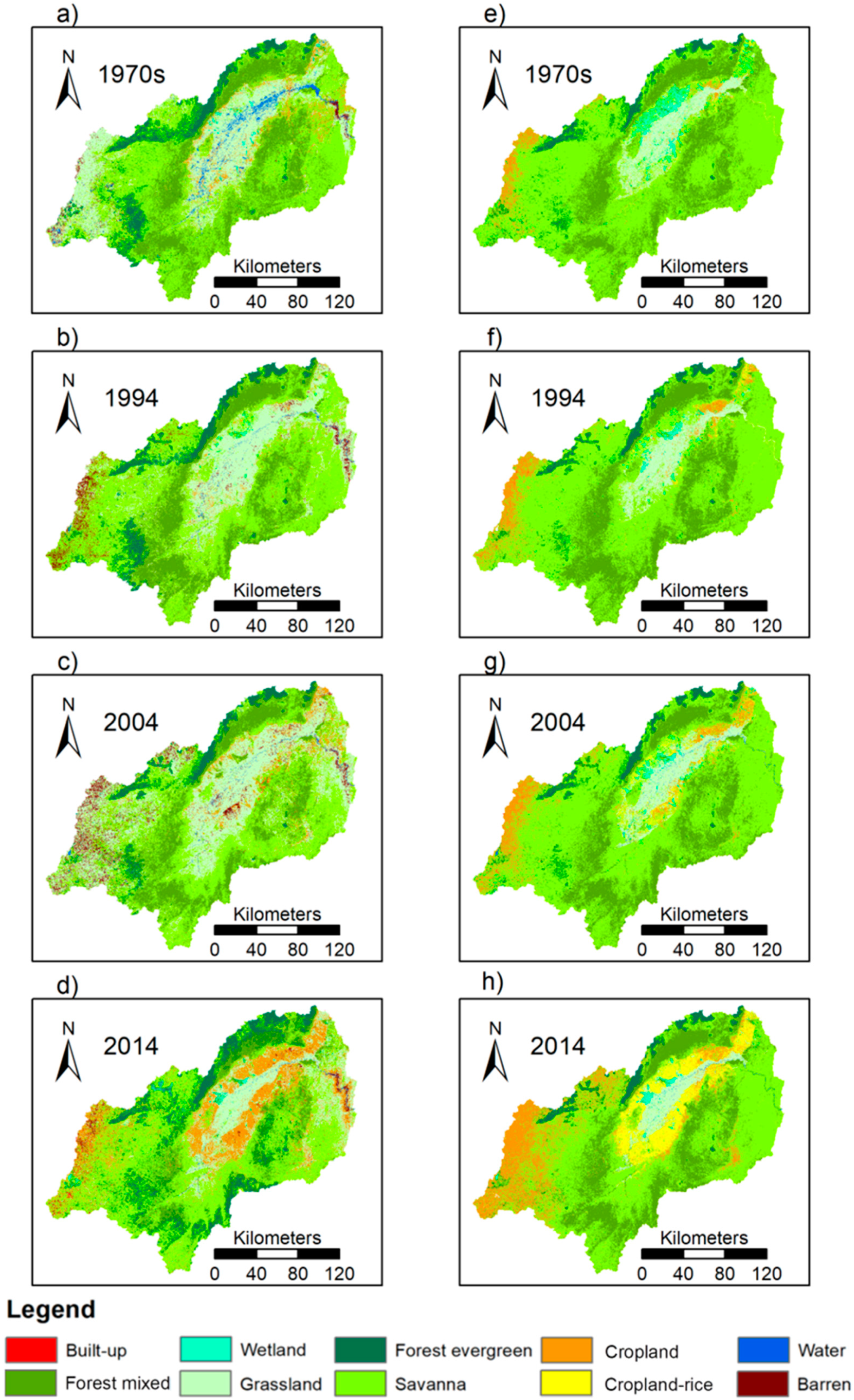
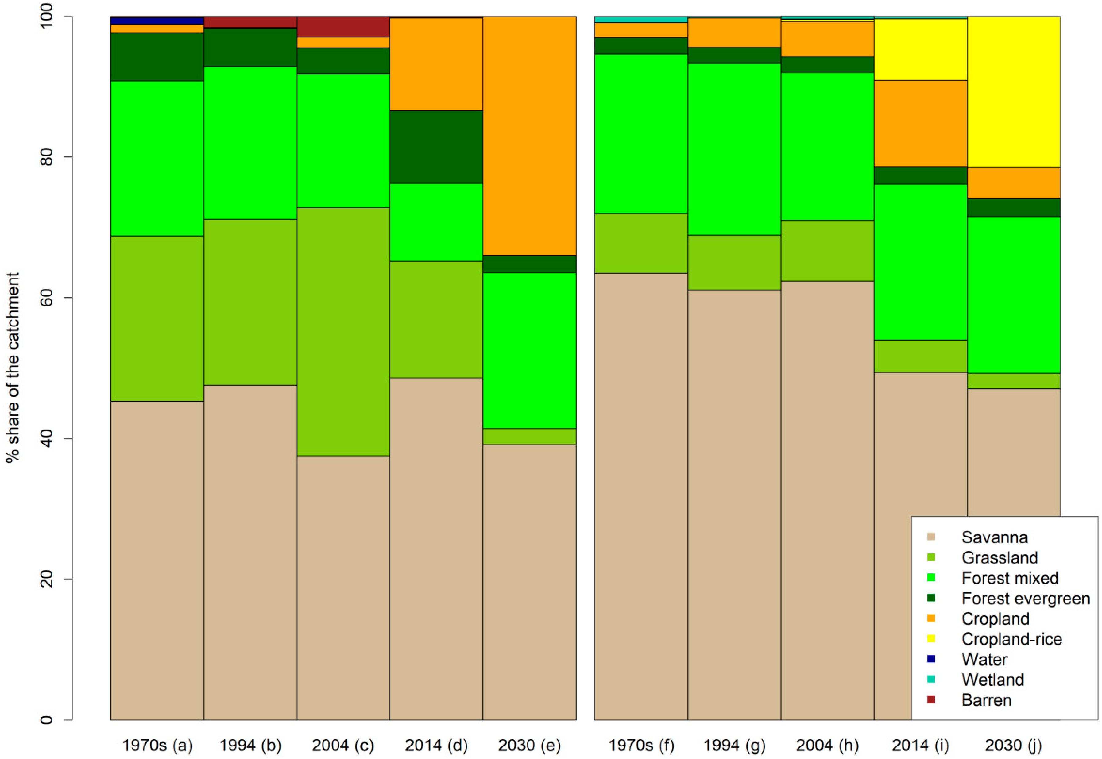
3.2. Land Use Land Cover Change Scenarios

Figure 4 shows the result of the LCM for the year 2030. The maps show increasing density of agricultural activities at the fringe of the floodplain and an agricultural encroachment towards the river, whereas the central part of the floodplain is not converted. Other hot spots of change are the western parts of the catchment and the central northern parts, especially in Figure 4c. Figure 4a,c also show agricultural activities in the eastern parts along the Kilombero River.

The percent share for all LULC types in the maps of Figure 2 and Figure 4 are displayed in Figure 5. The generic cropland setup distributions are shown on the left-hand side of Figure 5a–e and the maps with the differentiation of cropland and cropland-rice are displayed to the right-hand side of Figure 5f–j. The increasing share of cropland and cropland-rice classes from 2004 onwards for both setups is noteworthy. The share of forest classes is quite stable, although there are fluctuations in between forest mixed and forest evergreen. The decreasing trend of savanna in the cropland-rice setup from 2004 is remarkable and more pronounced than in the cropland setup. However, the cropland setup generally has a higher share of grassland and a strongly declining share of grassland from 2004 onwards. Other classes are much less represented or disappear in the final HRU setup like the built-up class. However, the distribution of the HRU setup reflects the original LULC distribution well. The disappearance of the built-up class in the HRU setups can be attributed to the low share of residential areas (<0.6%) in the baseline LULC setups from 1970 to 2014.

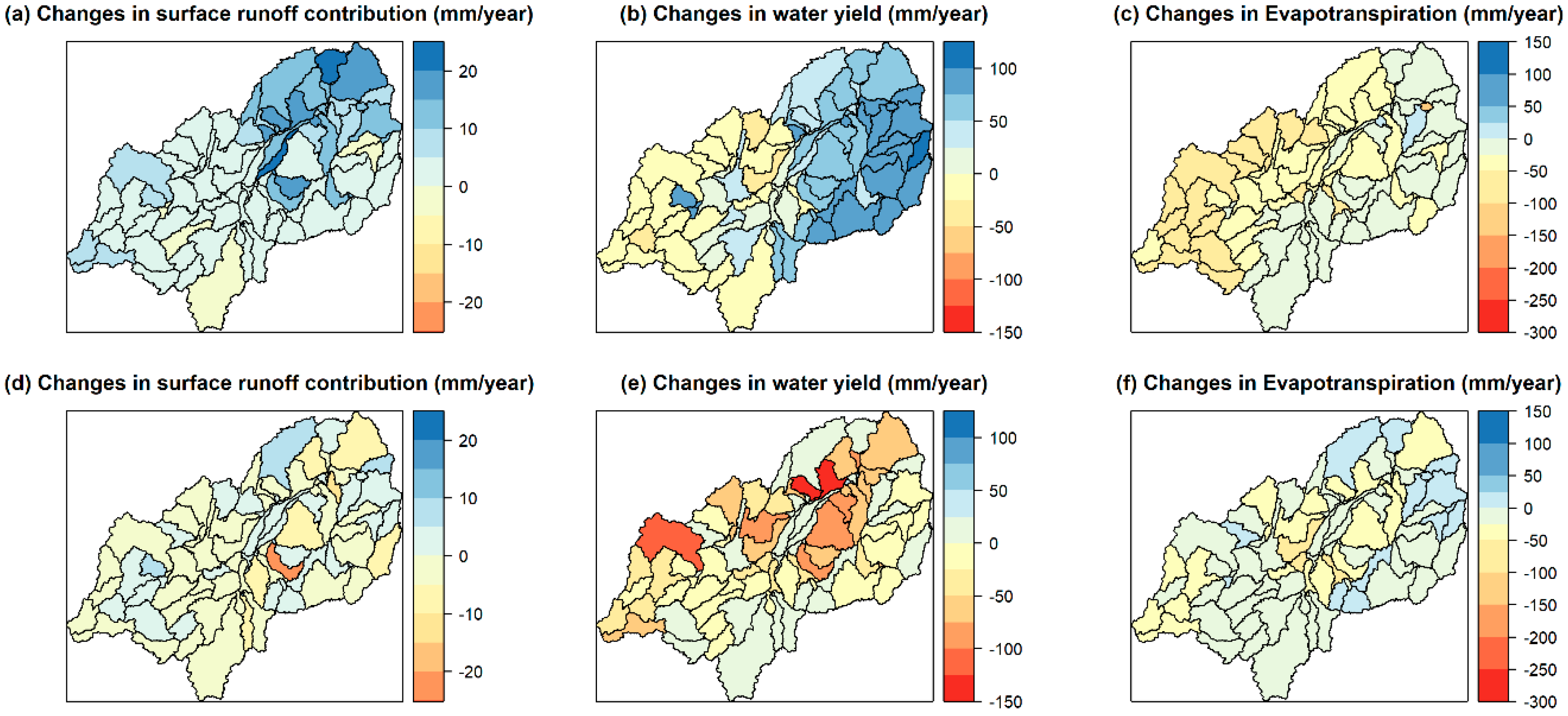
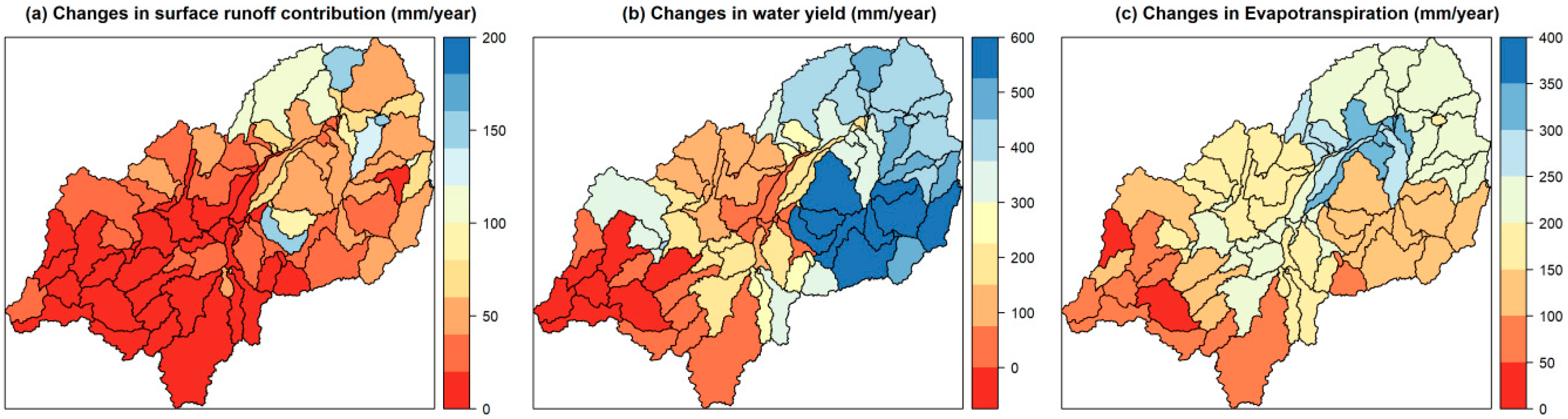
3.3. Impact of Land Use/Cover Changes on Water Resources

Figure 6a,b show that the overall annual discharge at the outlet is similar among all LULC setups. Nevertheless, a closer look at Figure 6c,d, which shows a zoom-in to the boxes, reveals differences between the two setups. On the one hand, the cropland setup (Figure 6c) shows an increasing trend for discharge from 1970 to 2030 with some fluctuations. These fluctuations are also reflected in fluctuations among the LULC classes in Figure 4. On the other hand, the setups that include rice (Figure 6d) show a constantly decreasing trend of discharge at the outlet with an increasing share of rice (Figure 5).

Figure 7 focuses on low flows (Figure 7a) and high flows (Figure 7b) for all setups. The general pattern for the low flows shows decreasing trends for the LULC setups including rice from the 1970s (Q90 of 119 m³/s) to 2030 (Q90 of 112 m³/s), which equals a drop of 6%. The cropland setups lack this trend, however the lowest Q90 value is again with the 2030 setup (114 m³/s). The values for Q10 show an analogous picture for the cropland-rice setup, with decreasing trends from the 1970s setup (1430 m³/s) to the 2030 setup (1320 m³/s). The absolute changes (110 m³/s) are more pronounced compared to the Q90 decrease, but the relative changes are comparable with 8%. The cropland setups show a different picture, with rather low absolute Q10 values from the 1970s (1118 m³/s) up to 2014 (1169 m³/s) and a sharp increase for the 2030 setup (1358 m³/s), which equals an increase of 21% compared to the 1970s setup.

Figure 8 shows the discharge amount for return levels for all setups based on the GEV-GMLE analysis of 48 annual maximum values from the period of 1958 to 2005. The distribution is similar to the Q10 values presented in Figure 7b. The discharge of 2-year and 5-year return levels for the cropland setups increase from the 1970s setup (3260 m³/s; 6310 m³/s) to the 2030 setup (3566 m³/s; 6595 m³/s), whereas the cropland-rice setups show an opposing trend (1970s: 3655 m³/s; 6663 m³/s; 2030: 3472 m³/s; 6437 m³/s). These trends are overcome by increasingly high return level values for both 2004 and 2014 setups. Furthermore, the relation of increasing return levels for the comparison of the 1970s setup and the 2030 setup with cropland is inverted from the 25-year return level onwards.

Figure 9 illustrates changes among LULC setups for selected water balance components, namely surface runoff, overall water yield and evapotranspiration on a monthly timescale for the whole simulation period from 1958–2005. All changes represent differences among the presented LULC setup and the basic setup from the 1970s. Hereby, all cropland setups (Figure 9a–d) are compared to the cropland 1970s setup and all cropland and cropland-rice setups (Figure 9e–h) are compared to the cropland and cropland-rice setup from the 1970s. Overall, the monthly changes are rather small, although water yield increases in the 2030 setup (Figure 9d) by an average of 22.3 mm per year in April, which equals 28.2% of the overall water yield for that month. Furthermore, evapotranspiration decreases nearly the whole year round (except for May and June) in that setup by up to 8.2 mm in average for the month of December, which equals 8.5% of the average evapotranspiration in that month. A different picture is shown for the rice scenarios (Figure 9e–h), where overall water yield decreases in the 2014 (Figure 9g) and 2030 (Figure 9h) setup for April and May. However, the average decrease ranges from 5.4 mm (5.1%; May, 2014 setup) to 8.1 mm (7.6%; May, 2030 setup) and is therefore less pronounced compared to the increases in the 2030 cropland setup.

Variations of surface runoff, overall water yield, and evapotranspiration on subcatchment scale are shown in Figure 10. Figure 10a–c compares the annual water balance components’ averages from the 2030 setup with the 1994 setup with cropland and Figure 10d–f compares the same with the cropland-rice setups, respectively. An increase of surface runoff and overall water yield is apparent (Figure 10a,b). The northeastern parts, and also the floodplain show increasing surface runoff values of 10 to 20 mm and increase in total water yield of more than 50 mm. Hence, evapotranspiration is decreasing in nearly all subcatchments, especially in the mountainous northwestern parts. The differences in the rice setups (Figure 10d–f) from 1994 to 2030 show a different pattern. Changes in surface runoff are less pronounced and most subcatchments show a slightly decreasing trend. Overall water yield is decreasing in many subcatchments by 50 mm and more, especially in the fringe of the floodplain, but also in some of the northwestern mountainous subcatchments. Furthermore, evapotranspiration is decreasing in many subcatchments, especially on the fringe of the floodplain and the western parts. However, slightly increasing trends of evapotranspiration are apparent e.g., in the northeastern subcatchments.

3.4. Combined Effect of Land Use/Cover and Climate Change on Water Resources

The combined effect of LULCC and climate change on water resources is illustrated for a combination of distinctive wet and dry model combinations in Figure 11 and Figure 12 in order to demonstrate the uncertainty and the span of possible future conditions according to the model combinations and their impact on water resources. Figure 11 displays the Q90 (Figure 11a) and Q10 (Figure 11b) modeling results for both LULC setups of 1994 and 2030, all driven by the climatic forcing of the “dry model” and the “wet model”. Apparently, the span for Q10 and Q90 of the “dry model” and the “wet model” is more pronounced in comparison to the differences among the LULC setups. The range of Q90 straddles from 101 m³/s (2030, rice, “dry model”) to 162 m³/s (1994, cropland, “wet model”). For Q10 the results span from 1310 m³/s (1994, cropland, “dry model”) to 2416 m³/s (1994, cropland-rice, “wet model”). These discrepancies represent a relative growth of 61% for Q90 and 84% for Q10, indicating a huge uncertainty for the future low flows and high flows with regard to a changing climate and LULCC. Furthermore, it is important to mention that all combined LULC and climate change scenarios for Q10 Figure 11b) show increasing values for Q10 compared to the LULC scenarios (Figure 7b), whereas Q90 values (Figure 7a) are lower for the dry climate scenario and higher for the wet climate scenario (Figure 11a).

Figure 12 illustrates a spatially more explicit dimension for the subcatchment scale by visualizing the deviations in surface runoff (Figure 12a), overall water yield (Figure 12b) and evapotranspiration (Figure 12c) between the cropland model setup of 1994 driven by the “dry model” and the cropland setup of 2030 driven by the “wet model”. The surface runoff component increases by more than 100 mm for some of the subcatchments in the annual average for the whole catchment and particularly for some of the subcatchments in the (north-) eastern part of the catchment. Unlike the western parts, which are mostly within the range of 0–20 mm increase. The pattern of the overall water yield is alike; however, it has another scale straddling from slightly decreasing trends in the western subcatchments to increasing values of nearly 600 mm in the eastern subcatchments. Water yield deviations increase towards the eastern parts, except for the floodplain, where this pattern is not as distinctive as for the surrounding mountainous areas. Evapotranspiration (Figure 12c) increases as well in the range of 100–200 mm for nearly all subcatchments and particularly for the northeastern floodplain and its fringe.

4. Discussion

4.1. Land Use Change Scenarios

This study focuses on changes from all LULC classes except built-up areas to either cropland or cropland-rice, although local studies in the catchment indicate the problem of deforestation as well [28]. However, deforestation is not as pronounced for the entire catchment (Figure 4) [1] and therefore only changes into agricultural LULC classes were explicitly modeled. Nevertheless, difficulties in the classification scheme among the different forest classes and open forest areas or savanna were apparent [2]. Natural classes in particular were prone to errors due to gradual differences in reflectance characteristics, although post-classification comparisons were mostly consistent and conform to historical maps. Yet, conversion into cropland was the focal LULCC and less prone to errors due to strong spectral changes [2]. Skill measures (Table 6) for both transitions to cropland or rice were satisfactory, nevertheless the exact distribution of LULC pixels in the 2030 scenarios should be interpreted carefully for several reasons. Firstly, the computed rate of change from 2004 to 2014 was transferred linearly until 2030. Secondly, this analyzed pattern is based on explanatory spatial factors like the altitude above sea level. Therefore, a saturation effect might occur due to limited space, e.g., in the wetland fringes surrounding the floodplain. The wetland fringes are nearly completely used as agricultural land in the setups of 2014 and 2030 (Figure 4). A growing demand for agricultural land in this area is a source of uncertainty, because the interaction with the enclosing landscape, and therefore agriculturally less suitable areas like upland forests or flood-prone areas, is a different process compared to the observed LULCC in the wetland fringes. Thirdly, alterations in demographic growth including natural birth rates and immigration are not included in this linear approach. However, the impacts of demographic growth on LULCC are indirectly integrated due to the transfer of observed changes from 2004 to 2014 to the year 2030. The demographic growth accelerated in the 90s and after 2000 due to the migration of mainly pastoralists into the valley [23] and correlates with the growing share of cropland in the valley, which was increasingly converted from grassland and savanna into cropland to feed the growing population. We use these conversions into cropland as a proxy for demographic growth, due to the stagnating trends in rice yields in the area [73,74], although conversions into cropland might also be affected by investors from outside the valley and other factors. Lastly, the influence of politics and the economy is not included, but might change the LULC drastically by setting incentives for agricultural activities e.g., the SAGCOT initiative [22], changing the allocation or status of conservation areas or by developing the infrastructure. Furthermore, the spatial structure of the SWAT model and its HRU approach, which summarizes results for HRUs and neglects interactions among neighboring grid-cells within a subcatchment [75], has structural limitations compared to a fully distributed grid-based solution. However, SWAT is a well proven tool to determine impacts on water resources due to LULCC [76,77,78]. Analysis of impacts on water resources on grid-cell scale is not the goal of this study, but rather to identify general trends of LULCC and their impact on specific areas prone to these LULCC in order to assist the local water resource management authorities to enable a sustainable use of the available water resources. Hence, a business as usual scenario until 2030 was developed using the LCM and all analyses with regard to water resources were performed from catchment to the subcatchment scale.

The general distribution and spread of the modeled cropland/rice production area is reasonable. The hot spot of change for both scenarios is the fringe of the wetland. However, the center of the wetland is not transformed to agricultural fields on both setups, which is also reasonable due to the extended flooding and the threat to lose the harvest [79]. Other areas of agricultural expansion are the western parts and the central northern parts, near the cities of Makambako and Njombe, and the main roads A104 and B4 (Figure 1). Although some rice is grown in the Njombe region, it is mainly an important production region for maize, Irish potato, tea, and flowers and therefore it is rather unlikely to dispense the income within these agriculturally suitable value chains for less suitable large scale rice production in this region. The southern part, which expanded from 2014 to the 2030 setups, was already confirmed by local experts in a participatory mapping exercise as a recent rice growing area in the framework of a stakeholder workshop in February 2019. The transformation of cropland to cropland-rice in the very northeastern parts is unlikely due to the existing and growing sugarcane fields of the Kilombero Sugar Company.

4.2. Land Use/Cover and Climate Change Impact Assessment on Water Resources

The impact of LULCC on average stream discharge seems to be negligible at the first glance (Figure 5). This is also in line with a former study on historical LULCC on cropland [2], and was also observed in another catchment in Tanzania [80] as well as in small catchments in West Africa with conversion of savanna into rice [81]. One important factor for the low impact at the main outlet is also the stable share and distribution of forest classes in the upland of the catchment (Figure 2, Figure 4 and Figure 5 and reference [2]). Yet, LULCC are still seen as the main driver for decreasing streamflow in Eastern and Southern Africa [82]. These minor changes in streamflow at the main outlet due to LULCC detected in this study can be attributed to concealing effects for large catchments [83] like the Kilombero Catchment. Therefore, it is important to analyze the water balance on several spatio-temporal scales like the subcatchment scale or monthly averages and also analyze changes in low- or high-flow patterns.

The Q90 as representative index for the low flows decreases for both scenarios—the cropland and the cropland-rice scenarios—by 6% or 8%, respectively, from 1970s to 2030. An environmental flow assessment found several parts of the catchment to be differently vulnerable to decreases in mean annual flows [36]. The upstream margin of the floodplain with a monthly recommended flow of 82.3% of the mean annual flow was defined as highly vulnerable concerning environmental flows [36]. Therefore, these decreasing trends of 6% and 8% of the Q90 at the outlet should be considered carefully for further analyses. Stakeholder interviews and discussions with local farmers revealed, that perennial tributaries of the Kilombero in the northeastern part of the catchment turned into seasonal tributaries in the last decades. This change is attributed to deforestation activities and expansion of cropland, and therefore needs to be taken seriously to maintain the socio-ecological system that depends on continuous availability of water resources and the transported sediments and attached nutrients [28,35].

High flows are more distinct in the rice scenarios (Figure 6), although they decrease with an increasing share of rice (Figure 7b), especially in the months of April and May (Figure 9g,h). The general differences among the cropland and cropland-rice scenarios arise from their different shares of all LULC classes (Figure 5). The rice setups have a lower share of forest classes for example and therefore a comparison that aims to determine the impact of a growing agricultural share should be done separately within the cropland-rice or cropland setups. Though, the decreasing high flows within the rice scenarios (Figure 6) can be attributed to the high water requirements of the rice plants [29].

The cropland scenario for 2030 (Figure 7b) displays a strong increase in the discharge amount of Q10, which is distributed to the months of March to May (Figure 9d). This might lead to aggravated flooding events, which could either endanger the farmer’s harvest [73,74] their lives, critical infrastructure and their livelihood [84]. Especially newly promoted, high yielding, but low growing improved varieties such as like SARO5 (TXD 306) might be negatively affected by these changes. These strong increases of water yield are accompanied by slightly decreasing evapotranspiration throughout the year (Figure 9d). These patterns with regard to LULCC and Q10 are aggravated by the effects of climate change. The combined effect of climate change and LULCC inherits an increase of 84% between the two scenarios comparing the lowest (LULC 1994, RCP4.5, dry model) and the highest (LULC 2030, RCP8.5, wet model) value for Q10 shown in Figure 11b. The effect of climate change outperforms the impact of LULCC, yet the contribution of LULCC to changes in Q10 is still substantial (Figure 7b). It is necessary to add that changes in management practices are not included in these LULCC, but several practices, like the establishment of year-round irrigation schedules, will further affect water resources [85,86]. Furthermore, the uncertainty of the climate change signal, represented by the huge span in the GCM-RCM model runs [33] (Figure 11), is much higher than in LULCC scenarios. While climate change models show diverging trends of more dry or more wet conditions and changes in the seasonality, the impact of conversion from natural LULC into agricultural utilized fields is more explicit [3,4,81], although it still depends on the specific crops grown. Nevertheless, intensification of precipitation might foster groundwater recharge and therefore access to renewable water resources in the Kilombero Catchment as well as already described in other catchments in SSA [87]. This indicates a particular resilience to climate change and intensification of precipitation events. However, more observation-driven research is needed on the relation of surface water and groundwater resources on this topic [87]. Moreover, data availability on the hydrogeology of the Kilombero Catchment is still poor to be modeled precisely, although some data and a local conceptual model exists [88,89]. Furthermore, the groundwater routines of the SWAT model are not sufficient for adequately modeling groundwater processes, because distributed parameters like the hydraulic conductivity and storage coefficients are disregarded in the linear reservoir approximations [90].

Overall, analyses on subcatchment scale (Figure 10 and Figure 12) show that the conversion into cropland leads to increasing surface runoff and overall water yield (Figure 10a,b), whereas a more diverse picture is shown for the rice setups (Figure 10d,e), due to the differences in LULC in the setups (Figure 5) and the aforementioned water demand of rice plants [29]. Average annual evapotranspiration is decreasing in both agricultural setups in most of the subcatchments, especially where natural systems are converted into agricultural production zones, which is in line with other studies from the tropics [3,6,7]. Still, there are studies that report increasing evapotranspiration due to conversion of forests to cropland [91]. However, farming in the Kilombero Catchment is mainly done by low input rain-fed rice cultivation and only a few rice irrigation schemes do exist [92]. Therefore, the rice setups were established using the default management plan from SWAT. A high input management setup would change the plant growth and consequently the evaporation of the plants [81].

The scale dependency of hydrological processes and the spatio-temporal heterogeneity of water movement within the catchment are apparent by comparing the different characteristics of selected water balance components in the subcatchments (Figure 10 and Figure 12) and their monthly deviations for the entire catchment (Figure 9 and reference [2]). The deviations that include the effects of climate change (Figure 12) are substantial, even though they compare the extreme situations concerning LULCC and climate change scenarios.

The manifold scenarios, inherited uncertainties and their implications on water resource management reveal the difficulties for local authorities and the need for further research in the area. The population in the catchment districts Kilombero and Ulanga has been and is currently increasing [47] and road infrastructure as well as the Stiegler’s Gorge power station are being constructed. This will lead to further LULCC, and locally rapid deforestation has already been reported [28,93], consequently affecting the water balance [94]. Forest protection against unregulated degradation is still problematic in Tanzania. There is a need to understand the social-ecological system to strengthen strategies, that ensure socio-economic benefits of local people, while preventing ecosystem degradation to allow a sustainable utilization and protection of the resource base [5]. The local scale and the understanding of the local communities that depend on the wetland resources and their adjacent mountain forests and savannas could be the key for the development of management policies in the Kilombero Catchment [95]. These could be for example the promotion of environmentally friendly sources of livelihood such as beekeeping, a sustainable forestry system accompanied by education on the socio-ecological system and improvements in the agricultural practices [23]. Still, migration into the valley and population growth are critical factors for the pressure on the ecological system [23,95,96]. Further information on the flooding extent, timing and duration using a hydraulic model with regard to the LULCC and climate change scenarios should support to manage the floodplain under future conditions. Beyond that, there is still not sufficient data on water quality, especially with regard to the emerging use of fertilizers, herbicides, and pesticides [35,95].

5. Conclusions

The study shows different methods to develop LULC maps and how to utilize these methods for further LULC scenario development. Differences among these scenarios and their effects on water resources are shown. However, implications of LULCC and climate change impacts on various spatio-temporal scales are key aspects of this study. Results clearly show that it is not sufficient to analyze discharge only at the outlet in LULCC impact studies [97]. It was shown that further analyses on different spatial scales and changes in low flows and high flow behavior are essential to identify hot spots of change, obtain environmental flows and for flood protection. The scenario analysis shows a trend of decreasing low flows, especially until 2030 by 6% to 8%. These numbers should be taken seriously, as they represent only the catchment´s average, while several areas, e.g., the northwestern parts, show more pronounced declines in overall water yield and evapotranspiration. Since some rivers in the northwest that have already been subject to a shift from perennial to seasonal rivers management activities are crucial to maintaining and protecting the system. This study helps to identify areas that are essential for the maintenance of the social-ecological system with regard to water resources. However, these activities have to take part in collaboration with the involvement of local communities and might need the establishment of local management authorities to enable a sustainable management of the catchment [34]. Potential management activities could contain the protection of natural swamps within the valley or upland forests in combination with payment for ecosystem services to incentivize these protection zones for local communities. Other options include the exploration of more environmental friendly activities such as beekeeping or more sustainable forestry systems [23]. Additionally, information with regard to the endangered ecosystems and their importance for the farmer’s fields should be communicated e.g., through extension officers to create mutual acceptance for these protection zones.

Conversely, high flows are more pronounced for the overall catchment with an increase of Q10 by up to 21% in 2030 compared to the 1970s due to LULCC only. These increases are associated with the months of March to May (the rainy season) and are remarkable for the town of Ifakara—a highly populated area with many small scale farmers, that frequently uses high yielding, but low growing rice varieties. Hence, the livelihood of the population in that area is at risk due to these LULCC, which are particularly fostered by climate change. Therefore, the retention capacities of natural systems like forests or swamps are indispensable for the maintenance of the social-ecological system.

Further analysis with specific crop and rice management parameterizations are recommended for more accurate projections. These projections should be utilized to run a hydraulic model for the flood areas in order to assist sustainable management with regard to water resources. The results of this study indicate a strong impact of changing climate on the water cycle, whereas the conversion of predominantly savanna and grassland to agricultural areas is less dramatic, yet remains important at the subcatchment scale.

References

1. Leemhuis, C.; Thonfeld, F.; Näschen, K.; Steinbach, S.; Muro, J.; Strauch, A.; López, A.; Daconto, G.; Games, I.; Diekkrüger, B. Sustainability in the food-water-ecosystem nexus: The role of land use and land cover change for water resources and ecosystems in the Kilombero Wetland, Tanzania. Sustainabiliyr 2017, 9, 1513. [Google Scholar] [CrossRef] [Green Version]
2. Näschen, K.; Diekkrüger, B.; Leemhuis, C.; Steinbach, S.; Seregina, L.; Thonfeld, F.; van der Linden, R. Hydrological Modeling in Data-Scarce Catchments: The Kilombero Floodplain in Tanzania. Water 2018, 10, 599. [Google Scholar] [CrossRef] [Green Version]
3. Yira, Y.; Diekkrüger, B.; Steup, G.; Bossa, A.Y. Modeling land use change impacts on water resources in a tropical West African catchment (Dano, Burkina Faso). J. Hydrol. 2016, 537, 187–199. [Google Scholar] [CrossRef]
4. Op de Hipt, F. Modeling Climate and Land Use Change Impacts on Water Resources in the Dano Catchment. Ph.D. Thesis, University of Bonn, Bonn, Germany, 2018. [Google Scholar]
5. Rosa, I.M.D.; Rentsch, D.; Hopcraft, J.G.C. Evaluating forest protection strategies: A comparison of land-use systems to preventing forest loss in Tanzania. Sustainability 2018, 10, 4476. [Google Scholar] [CrossRef]
6. Gabiri, G.; Leemhuis, C.; Diekkrüger, B.; Näschen, K.; Steinbach, S.; Thonfeld, F. Modelling the impact of land use management on water resources in a tropical inland valley catchment of central Uganda, East Africa. Sci. Total Environ. 2019, 653, 1052–1066. [Google Scholar] [CrossRef]
7. Guzha, A.C.; Rufino, M.C.; Okoth, S.; Jacobs, S.; Nóbrega, R.L.B. Impacts of land use and land cover change on surface runoff, discharge and low flows: Evidence from East Africa. J. Hydrol. Reg. Stud. 2018, 15, 49–67. [Google Scholar] [CrossRef]
8. Mucova, S.A.R.; Filho, W.L.; Azeiteiro, U.M.; Pereira, M.J. Assessment of land use and land cover changes from 1979 to 2017 and biodiversity & land management approach in Quirimbas National Park, Northern Mozambique, Africa. Glob. Ecol. Conserv. 2018, 16, e00447. [Google Scholar]
9. Brink, A.B.; Eva, H.D. Monitoring 25 years of land cover change dynamics in Africa: A sample based remote sensing approach. Appl. Geogr. 2009, 29, 501–512. [Google Scholar] [CrossRef]
10. Brink, A.B.; Bodart, C.; Brodsky, L.; Defourney, P.; Ernst, C.; Donney, F.; Lupi, A.; Tuckova, K. Anthropogenic pressure in East Africa—Monitoring 20 years of land cover changes by means of medium resolution satellite data. Int. J. Appl. Earth Obs. Geoinf. 2014, 28, 60–69. [Google Scholar] [CrossRef]
11. Marchant, R.; Richer, S.; Boles, O.; Capitani, C.; Courtney-Mustaphi, C.J.; Lane, P.; Prendergast, M.E.; Stump, D.; De Cort, G.; Kaplan, J.O.; et al. Drivers and trajectories of land cover change in East Africa: Human and environmental interactions from 6000 years ago to present. Earth-Sci. Rev. 2018, 178, 322–378. [Google Scholar] [CrossRef]
12. Kleemann, J.; Baysal, G.; Bulley, H.N.N.; Fürst, C. Assessing driving forces of land use and land cover change by a mixed-method approach in north-eastern Ghana, West Africa. J. Environ. Manag. 2017, 196, 411–442. [Google Scholar] [CrossRef] [PubMed]
13. Meijer, J.; Shames, S.; Scherr, S.J.; Giesen, P. Spatial Scenario Modelling to Support Integrated Landscape Management in the Kilombero Valley Landscape in Tanzania; PBL Netherlands Environmental Assessment Agency: The Hague, The Netherlands, 2018. [Google Scholar]
14. Nhemachena, C.; Matchaya, G.; Nhemachena, C.; Karuaihe, S.; Muchara, B.; Nhlengethwa, S. Measuring Baseline Agriculture-Related Sustainable Development Goals Index for Southern Africa. Sustainability 2018, 10, 849. [Google Scholar] [CrossRef] [Green Version]
15. Faramarzi, M.; Abbaspour, K.C.; Ashraf Vaghefi, S.; Farzaneh, M.R.; Zehnder, A.J.B.; Srinivasan, R.; Yang, H. Modeling impacts of climate change on freshwater availability in Africa. J. Hydrol. 2013, 480, 85–101. [Google Scholar] [CrossRef]
16. Op de Hipt, F.; Diekkrüger, B.; Steup, G.; Yira, Y.; Hoffmann, T.; Rode, M.; Näschen, K. Modeling the impact of climate change on water resources and soil erosion in a tropical catchment in Burkina Faso, West Africa. Sci. Total Environ. 2019, 653, 431–445. [Google Scholar] [CrossRef]
17. Notter, B.; Hurni, H.; Wiesmann, U.; Ngana, J.O. Evaluating watershed service availability under future management and climate change scenarios in the Pangani Basin. Phys. Chem. Earth 2013, 61–62, 1–11. [Google Scholar] [CrossRef]
18. Funk, C.; Dettinger, M.D.; Michaelsen, J.C.; Verdin, J.P.; Brown, M.E.; Barlow, M.; Hoell, A. Warming of the Indian Ocean threatens eastern and southern African food security but could be mitigated by agricultural development. Proc. Natl. Acad. Sci. USA 2008, 105, 11081–11086. [Google Scholar] [CrossRef] [Green Version]
19. Williams, A.P.; Funk, C. A westward extension of the warm pool leads to a westward extension of the Walker circulation, drying eastern Africa. Clim. Dyn. 2011, 37, 2417–2435. [Google Scholar] [CrossRef] [Green Version]
20. Shongwe, M.E.; van Oldenborgh, G.J.; van den Hurk, B.; van Aalst, M.; Shongwe, M.E.; Oldenborgh, G.J.; van den Hurk, B.; van Aalst, M. Projected Changes in Mean and Extreme Precipitation in Africa under Global Warming. Part II: East Africa. J. Clim. 2011, 24, 3718–3733. [Google Scholar] [CrossRef] [Green Version]
21. Lyon, B.; DeWitt, D.G. A recent and abrupt decline in the East African long rains. Geophys. Res. Lett. 2012, 39, 1–5. [Google Scholar] [CrossRef] [Green Version]
22. Environmental Resources Management. Southern Agricultural Growth Corridor of Tanzania (SAGCOT): Environmental and Social Management Framework (ESMF); SAGCOT: Dar es Salaam, Tanzania, 2013. [Google Scholar]
23. Msofe, N.K.; Sheng, L.; Lyimo, J. Land use change trends and their driving forces in the Kilombero Valley Floodplain, Southeastern Tanzania. Sustainability 2019, 11, 505. [Google Scholar] [CrossRef] [Green Version]
24. Milder, J.C.; Hart, A.K.; Buck, L.E. Applying an Agriculture Green Growth Approach in the SAGCOT Clusters: Challenges and Opportunities in Kilombero, Ihemi and Mbarali; SAGCOT Centre Limited: Dar es Salaam, Tanzania, 2013. [Google Scholar]
25. Steffens, V.; Hartmann, G.; Dannenberg, P. Eine neue Generation von Wachstumskorridoren als Entwicklungsmotor in Afrika? Standort 2019, 43, 2–8. [Google Scholar] [CrossRef]
26. Muro, J.; Strauch, A.; Heinemann, S.; Steinbach, S.; Thonfeld, F.; Waske, B.; Diekkrüger, B. Land surface temperature trends as indicator of land use changes in wetlands. Int. J. Appl. Earth Obs. Geoinf. 2018, 70, 62–71. [Google Scholar] [CrossRef]
27. Kangalawe, R.Y.M.; Liwenga, E.T. Livelihoods in the wetlands of Kilombero Valley in Tanzania: Opportunities and challenges to integrated water resource management. Phys. Chem. Earth Parts A/B/C 2005, 30, 968–975. [Google Scholar] [CrossRef]
28. Johansson, E.L.; Abdi, A.M. Mapping and quantifying perceptions of environmental change in Kilombero Valley, Tanzania. Ambio 2019, 1–12. [Google Scholar] [CrossRef] [PubMed] [Green Version]
29. Duku, C.; Zwart, S.J.; Hein, L. Modelling the forest and woodland-irrigation nexus in tropical Africa: A case study in Benin. Agric. Ecosyst. Environ. 2016, 230, 105–115. [Google Scholar] [CrossRef]
30. Eastman, J.R. TerrSet Tutorial: Geospatial Monitoring and Modeling System; Clark University: Worcester, MA, USA, 2016. [Google Scholar]
31. Mas, J.-F.; Kolb, M.; Paegelow, M.; Camacho Olmedo, M.T.; Houet, T. Inductive pattern-based land use/cover change models: A comparison of four software packages. Environ. Model. Softw. 2014, 51, 94–111. [Google Scholar] [CrossRef] [Green Version]
32. Eastman, J.R. TerrSet Manual. Geospatial Monitoring and Modeling System; Clark University: Worcester, MA, USA, 2016. [Google Scholar]
33. Näschen, K.; Diekkrüger, B.; Leemhuis, C.; Seregina, L.S.; Linden, R. van der Impact of Climate Change on Water Resources in the Kilombero Catchment in Tanzania. Water 2019, 11, 859. [Google Scholar] [CrossRef] [Green Version]
34. Daconto, G.; Games, I.; Lukumbuzya, K.; Raijmakers, F. Integrated Management Plan for the Kilombero Valley Ramsar Site; Ministry of Natural Resources and Tourism: Dar es Salaam, Tanzania, 2018.
35. Wilson, E.; McInnes, R.; Mbaga, D.P.; Ouedaogo, P. Ramsar Advisory Mission Report: United Republic of Tanzania, Kilombero Valley; Ramsar Secretariat: Gland, Switzerland, 2017. [Google Scholar]
36. CDM Smith. Environmental Flows in Rufiji River Basin Assessed from the Perspective of Planned Development in Kilombero and Lower Rufiji Sub-Basins; Report to the United States Agency for International Development; US AID: Dar es Salaam, Tanzania, 2016.
37. Mombo, F.; Speelman, S.; Van Huylenbroeck, G.; Hella, J.; Moe, S. Ratification of the Ramsar convention and sustainable wetlands management: Situation analysis of the Kilombero Valley wetlands in Tanzania. J. Agric. Ext. Rural Dev. 2011, 3, 153–164. [Google Scholar]
38. Nindi, S.J.; Maliti, H.; Bakari, S.; Kija, H.; Machoke, M. Conflicts over Land and water resources in the Kilombero Valley Floodplain, Tanzania. Afr. Study Monogr. 2014, 50, 173–190. [Google Scholar]
39. Camberlin, P.; Philippon, N. The East African March–May Rainy Season: Associated Atmospheric Dynamics and Predictability over the 1968–97 Period. J. Clim. 2002, 15, 1002–1019. [Google Scholar] [CrossRef]
40. Zorita, E.; Tilya, F.F. Rainfall variability in Northern Tanzania in the March-May season (long rains) and its links to large-scale climate forcing. Clim. Res. 2002, 20, 31–40. [Google Scholar] [CrossRef]
41. Seregina, L.S.; Fink, A.H.; van der Linden, R.; Elagib, N.A.; Pinto, J.G. A new and flexible rainy season definition: Validation for the Greater Horn of Africa and application to rainfall trends. Int. J. Climatol. 2018, 39, 989–1012. [Google Scholar] [CrossRef]
42. Koutsouris, A.J.; Chen, D.; Lyon, S.W. Comparing global precipitation data sets in eastern Africa: A case study of Kilombero Valley, Tanzania. Int. J. Climatol. 2016, 36, 2000–2014. [Google Scholar] [CrossRef]
43. Nicholson, S.E. Climate and climatic variability of rainfall over eastern Africa. Rev. Geophys. 2017, 55, 590–635. [Google Scholar] [CrossRef] [Green Version]
44. Dewitte, O.; Jones, A.; Spaargaren, O.; Breuning-Madsen, H.; Brossard, M.; Dampha, A.; Deckers, J.; Gallali, T.; Hallett, S.; Jones, R.; et al. Harmonisation of the soil map of africa at the continental scale. Geoderma 2013, 211–212, 138–153. [Google Scholar] [CrossRef] [Green Version]
45. Zemandin, B.; Mtalo, F.; Mkhandi, S.; Kachroo, R.; McCartney, M. Evaporation Modelling in Data Scarce Tropical Region of the Eastern Arc Mountain Catchments of Tanzania. Nile Basin Water Sci. Eng. J. 2011, 4, 1–13. [Google Scholar]
46. Kato, F. Development of a major rice cultivation area in the Kilombero Valley, Tanzania. Afr. Study Monogr. 2007, 36, 3–18. [Google Scholar]
47. National Bureau of Statistics. 2012 Population and Housing Census Report; National Bureau of Statistics: Dar es Salaam, Tanzania, 2012. [Google Scholar]
48. RBWB. The Rufiji Basin Water Board (RBWB) Discharge Database; RBWB: Iringa, Tanzania, 2014. [Google Scholar]
49. Mack, B.; Leinenkugel, P.; Kuenzer, C.; Dech, S. A semi-automated approach for the generation of a new land use and land cover product for Germany based on Landsat time-series and Lucas in-situ data. Remote Sens. Lett. 2017, 8, 244–253. [Google Scholar] [CrossRef]
50. Breiman, L. Random forests. Mach. Learn. 2001, 45, 5–32. [Google Scholar] [CrossRef] [Green Version]
51. Gutowski, J.W.; Giorgi, F.; Timbal, B.; Frigon, A.; Jacob, D.; Kang, H.S.; Raghavan, K.; Lee, B.; Lennard, C.; Nikulin, G.; et al. WCRP Coordinated Regional Downscaling EXperiment (CORDEX): A diagnostic MIP for CMIP6. Geosci. Model Dev. 2016, 9, 4087–4095. [Google Scholar] [CrossRef] [Green Version]
52. Lehner, B.; Verdin, K.; Jarvis, A. New Global Hydrography Derived From Spaceborne Elevation Data. Eos Trans. Am. Geophys. Union 2008, 89, 93–104. [Google Scholar] [CrossRef]
53. United States Geological Survey (USGS). EarthExplorer. Available online: https://earthexplorer.usgs.gov/ (accessed on 8 December 2016).
54. USGS. Department of the Interior Product Guide–Landsat 4–7 Surface Reflectance (LEDAPS) Product Version 8.0. Available online: https://landsat.usgs.gov/sites/default/files/documents/ledaps_product_guide.pdf (accessed on 8 December 2016).
55. USGS. Department of the Interior Product Guide Landsat 8 Surface Reflectance Code (LASRC) Product Version 4.1. Available online: https://landsat.usgs.gov/sites/default/files/documents/lasrc_product_guide.pdf (accessed on 8 December 2016).
56. Arnold, J.G.; Srinivasan, R.; Muttiah, R.S.; Williams, J.R. Large area hydrologic modeling and assessment part I: Model development. J. Am. Water Resour. Assoc. 1998, 34, 73–89. [Google Scholar] [CrossRef]
57. Williams, J.R. The EPIC Model. In Computer Models of Watershed Hydrology; Water Resources Publications: Highlands Ranch, CO, USA, 1995; pp. 909–1000. [Google Scholar]
58. Neitsch, S.L.; Arnold, J.G.; Kiniry, J.R.; Williams, J.R. Soil & Water Assessment Tool Theoretical Documentation, version 2009; Neitsch, S.L., Arnold, J.G., Kiniry, J.R., Williams, J.R., Eds.; Grassland, Soil and Water Research Laboratory: Temple, TX, USA, 2011. [Google Scholar]
59. Soil Conservation Service (Ed.) Hydrology. In National Engineering Handbook; Soil Conservation Service: Lakewood, CO, USA, 1972. [Google Scholar]
60. Monteith, J.L.; Moss, C.J. Climate and the Efficiency of Crop Production in Britain. Philos. Trans. R. Soc. B Biol. Sci. 1977, 281, 277–294. [Google Scholar] [CrossRef]
61. Sloan, P.G.; Moore, I.D. Modeling subsurface stormflow on steeply sloping forested watersheds. Water Resour. Res. 1984, 20, 1815–1822. [Google Scholar] [CrossRef] [Green Version]
62. Liu, W.; Park, S.; Bailey, R.T.; Molina-Navarro, E.; Andersen, H.E.; Thodsen, H.; Nielsen, A.; Jeppesen, E.; Jensen, J.S.; Jensen, J.B.; et al. Comparing SWAT with SWAT-MODFLOW hydrological simulations when assessing the impacts of groundwater abstractions for irrigation and drinking water. Hydrol. Earth Syst. Sci. Discuss. 2019, 1–51. [Google Scholar] [CrossRef] [Green Version]
63. Arnold, J.G.; Kiniry, J.R.; Srinivasan, R.; Williams, J.R.; Haney, E.B.; Neitsch, S.L. Soil & Water Assessment Tool: Input/output Documentation; Texas Water Recources Institute: College Station, TX, USA, 2012. [Google Scholar]
64. Abbaspour, K.C. SWAT-CUP 2012. SWAT Calibration and Uncertainty Programs; Abbaspour, K.C., Ed.; Eawag: Dübendorf, Switzerland, 2013. [Google Scholar]
65. Gilleland, E.; Katz, R.W. extRemes 2.0: An Extreme Value Analysis Package in R. J. Stat. Softw. 2016, 72, 1–39. [Google Scholar] [CrossRef] [Green Version]
66. Smakhtin, V.U. Low flow hydrology: A review. J. Hydrol. 2001, 240, 147–186. [Google Scholar] [CrossRef]
67. van Vliet, M.T.H.; Franssen, W.H.P.; Yearsley, J.R.; Ludwig, F.; Haddeland, I.; Lettenmaier, D.P.; Kabat, P. Global river discharge and water temperature under climate change. Glob. Environ. Chang. 2013, 23, 450–464. [Google Scholar] [CrossRef]
68. Bond, N. Hydrostats: Hydrologic Indices for Daily Time Series Data, R package version 0.2.4. 16 October 2015.
69. Anand, J.; Gosain, A.K.; Khosa, R. Prediction of land use changes based on Land Change Modeler and attribution of changes in the water balance of Ganga basin to land use change using the SWAT model. Sci. Total Environ. 2018, 644, 503–519. [Google Scholar] [CrossRef]
70. Gashaw, T.; Tulu, T.; Argaw, M.; Worqlul, A.W. Modeling the hydrological impacts of land use/land cover changes in the Andassa watershed, Blue Nile Basin, Ethiopia. Sci. Total Environ. 2018, 619–620, 1394–1408. [Google Scholar] [CrossRef]
71. Adhikari, S.; Southworth, J.; Adhikari, S.; Southworth, J. Simulating Forest Cover Changes of Bannerghatta National Park Based on a CA-Markov Model: A Remote Sensing Approach. Remote Sens. 2012, 4, 3215–3243. [Google Scholar] [CrossRef] [Green Version]
72. Vogelmann, J.E.; Gallant, A.L.; Shi, H.; Zhu, Z. Perspectives on monitoring gradual change across the continuity of Landsat sensors using time-series data. Remote Sens. Environ. 2016, 185, 258–270. [Google Scholar] [CrossRef] [Green Version]
73. Duvail, S.; Hamerlynck, O. The Rufiji River flood: Plague or blessing? Int. J. Biometeorol. 2007, 52, 33–42. [Google Scholar] [CrossRef] [PubMed]
74. Kwesiga, J.; Grotelüschen, K.; Neuhoff, D.; Senthilkumar, K.; Döring, T.F.; Becker, M. Site and Management Effects on Grain Yield and Yield Variability of Rainfed Lowland Rice in the Kilombero Floodplain of Tanzania. Agronomy 2019, 9, 632. [Google Scholar] [CrossRef] [Green Version]
75. Rathjens, H.; Oppelt, N. SWATgrid: An interface for setting up SWAT in a grid-based discretization scheme. Comput. Geosci. 2012, 45, 161–167. [Google Scholar] [CrossRef]
76. Niraula, R.; Meixner, T.; Norman, L.M. Determining the importance of model calibration for forecasting absolute/relative changes in streamflow from LULC and climate changes. J. Hydrol. 2015, 522, 439–451. [Google Scholar] [CrossRef]
77. Cornelissen, T.; Diekkrüger, B.; Giertz, S. A comparison of hydrological models for assessing the impact of land use and climate change on discharge in a tropical catchment. J. Hydrol. 2013, 498, 221–236. [Google Scholar] [CrossRef]
78. Martinez-Martinez, E.; Nejadhashemi, A.P.; Woznicki, S.A.; Love, B.J. Modeling the hydrological significance of wetland restoration scenarios. J. Environ. Manag. 2014, 133, 121–134. [Google Scholar] [CrossRef]
79. Gabiri, G.; Burghof, S.; Diekkrüger, B.; Steinbach, S.; Näschen, K. Modeling Spatial Soil Water Dynamics in a Tropical Floodplain, East Africa. Water 2018, 10, 191. [Google Scholar] [CrossRef] [Green Version]
80. Wambura, F.J.; Dietrich, O.; Graef, F. Analysis of infield rainwater harvesting and land use change impacts on the hydrologic cycle in the Wami River basin. Agric. Water Manag. 2018, 203, 124–137. [Google Scholar] [CrossRef]
81. Danvi, A.; Giertz, S.; Zwart, S.J.; Diekkrüger, B. Rice intensification in a changing environment: Impact on water availability in inland valley landscapes in Benin. Water 2018, 10, 74. [Google Scholar] [CrossRef] [Green Version]
82. Schäfer, M.P.; Dietrich, O.; Mbilinyi, B. Streamflow and lake water level changes and their attributed causes in Eastern and Southern Africa: State of the art review. Int. J. Water Resour. Dev. 2016, 32, 853–880. [Google Scholar] [CrossRef]
83. Wagner, P.D.; Kumar, S.; Schneider, K. An assessment of land use change impacts on the water resources of the Mula and Mutha Rivers catchment upstream of Pune, India. Hydrol. Earth Syst. Sci. 2013, 17, 2233–2246. [Google Scholar] [CrossRef] [Green Version]
84. National Bureau of Statistics. The National Environment Statistics Report, 2017 (NESR, 2017)–Tanzania Mainland; National Bureau of Statistics: Dar es Salaam, Tanzania, 2017. [Google Scholar]
85. Reshmidevi, T.V.; Nagesh Kumar, D.; Mehrotra, R.; Sharma, A. Estimation of the climate change impact on a catchment water balance using an ensemble of GCMs. J. Hydrol. 2018, 556, 1192–1204. [Google Scholar] [CrossRef] [Green Version]
86. Reshmidevi, T.V.; Nagesh Kumar, D. Modelling the impact of extensive irrigation on the groundwater resources. Hydrol. Process. 2014, 28, 628–639. [Google Scholar] [CrossRef]
87. Cuthbert, M.O.; Taylor, R.G.; Favreau, G.; Todd, M.C.; Shamsudduha, M.; Villholth, K.G.; MacDonald, A.M.; Scanlon, B.R.; Kotchoni, D.O.V.; Vouillamoz, J.-M.; et al. Observed controls on resilience of groundwater to climate variability in sub-Saharan Africa. Nature 2019, 572, 230–234. [Google Scholar] [CrossRef]
88. Burghof, S.; Gabiri, G.; Stumpp, C.; Chesnaux, R.; Reichert, B. Development of a hydrogeological conceptual wetland model in the data-scarce north-eastern region of Kilombero Valley, Tanzania. Hydrogeol. J. 2017, 26, 267–284. [Google Scholar] [CrossRef]
89. Burghof, S. Hydrogeology and Water Quality of Wetlands in East Africa. Ph.D. Thesis, University of Bonn, Bonn, Germany, 2017. [Google Scholar]
90. Kim, N.W.; Chung, I.M.; Won, Y.S.; Arnold, J.G. Development and application of the integrated SWAT–MODFLOW model. J. Hydrol. 2008, 356, 1–16. [Google Scholar] [CrossRef]
91. Mango, L.M.; Melesse, A.M.; McClain, M.E.; Gann, D.; Setegn, S.G. Land use and climate change impacts on the hydrology of the upper Mara River Basin, Kenya: Results of a modeling study to support better resource management. Hydrol. Earth Syst. Sci. 2011, 15, 2245–2258. [Google Scholar] [CrossRef] [Green Version]
92. Kashenge, S.; Makoninde, E. Perception and Indicators of Climate Change, Its Impacts, Available Mitigation Strategies in Rice Growing Communities Adjoining Eastern Arc Mountains. Univers. J. Agric. Res. 2017, 5, 267–279. [Google Scholar]
93. Munishi-Kongo, S. Ground and Satellite-Based Assessment of Hydrological Responses To Land Cover Change in the Kilombero River Basin. Ph.D. Thesis, University of KwaZulu-Natal, Durban, South Africa, 2013. [Google Scholar]
94. Yang, W.; Long, D.; Bai, P. Impacts of future land cover and climate changes on runoff in the mostly afforested river basin in North China. J. Hydrol. 2019, 570, 201–219. [Google Scholar] [CrossRef]
95. Msofe, N.K. Socio-Ecological Drivers of Land Use Change and Wetland Conversion in Kilombero Valley Floodoplain, Tanzania. Am. J. Environ. Resour. Econ. 2019, 4, 1–11. [Google Scholar] [CrossRef] [Green Version]
96. Johansson, E.L.; Isgren, E. Local perceptions of land-use change: Using participatory art to reveal direct and indirect socioenvironmental effects of land acquisitions in Kilombero Valley, Tanzania. Ecol. Soc. 2017, 22, 1–12. [Google Scholar] [CrossRef] [Green Version]
97. Hrachowitz, M.; Savenije, H.H.G.; Blöschl, G.; McDonnell, J.J.; Sivapalan, M.; Pomeroy, J.W.; Arheimer, B.; Blume, T.; Clark, M.P.; Ehret, U.; et al. A decade of Predictions in Ungauged Basins (PUB)—A review. Hydrol. Sci. J. 2013, 58, 1198–1255. [Google Scholar] [CrossRef]
Figure 1. Overview map of the study area, including available precipitation and discharge stations (Swero). The estimated floodplain area is based on visual interpretation of Landsat images (modified after Näschen et al. 2018 [2]).
Sustainability 11 07083 g001
Figure 2. Land use and land cover classifications for four time steps ranging from the 1970s (a,e), 1994 (b,f), and 2004 (c,g) up to 2014 (d,h). Some differences among the LULC maps in the right and in the left column exist due to the classification process: Only the maps in the left column contain “barren” as a land use class, but they have only one LULC “cropland”, whereas the maps in the right column differentiate in between “cropland” and “cropland-rice” as a specific crop.
Sustainability 11 07083 g002
Figure 3. Flow chart indicating the major processes to generate the LULC maps for the 2030 scenarios.
Sustainability 11 07083 g003
Figure 4. Land use and land cover classifications as modeled by the Land Change Modeler for the year 2030. For better comparison (a,b) show the setups for 2014 from Figure 2, (c) displays the scenario based on the single cropland classification and (d) illustrates the same scenario but distinguishes between cropland and cropland-rice land use class.
Sustainability 11 07083 g004
Figure 5. Observed and modeled (2030 (e,j)) share of the land use/land cover (LULC) classes within the Kilombero Catchment. (ae) show the distribution from the 1970s to 2030 with a different classification method compared to (fj). The built-up class dropped out in the final LULC distribution due to the low share of residential areas and the application of the HRU approach.
Sustainability 11 07083 g005
Figure 6. Box plots showing the annual discharge at the main outlet for the simulated period of 1958–2005. (a) shows the discharge for the setups with cropland only and (b) for the setup with the differentiation of cropland and cropland–rice. (c,d) show the very same information as (a,b), but zoom-in to the values of the boxes.
Sustainability 11 07083 g006
Figure 7. Distribution of Q90 (a) and Q10 (b), representing the flow exceeded in 90% or 10% of the time for Q90 and Q10, respectively. The reddish columns on the left represent the setups with cropland, whereas the blueish columns on the right display the modeling results for the setup with cropland and cropland-rice differentiated. Data is based on simulations from the period 1958–2005 and all inputs except for the LULC maps are not modified.
Sustainability 11 07083 g007
Figure 8. Return levels and respective discharge of flood events for all LULC setups. Return levels represent the discharge at the outlet for a 2-year, 5-year, 10-year, 25-year, 50-year, and 100-year event according to the generalized extreme value (GEV) model and the generalized maximum likelihood estimation (GMLE) method from the period of 1958 to 2005.
Sustainability 11 07083 g008
Figure 9. Average shifts (in mm) in selected water balance components for the entire catchment within the period from 1958 to 2005 compared to the 1970s setup with cropland (ad), or cropland-rice (eh). All inputs except for the LULC maps are not modified.
Sustainability 11 07083 g009
Figure 10. Average annual changes in selected water balance components on subcatchment scale. (ac) compares the cropland LULC maps of 1994 and 2030, while (df) compares the cropland-rice LULC maps of 1994 and 2030 on. All model runs used identic climate data from 1958 to 2005 and differences in water balance components refer only to changes in LULC.
Sustainability 11 07083 g010
Figure 11. Bar plots showing the distribution of Q90 (a) and Q10 (b), representing the flow exceeded in 90% or 10% of the time for Q90 and Q10, respectively. The LULC setups of 1994 (cropland and cropland-rice) as well as the scenarios for 2030 (cropland and cropland-rice) are simulated with climate data of the period from 2010 to 2060 with the “dry” and the “wet” GCM-RCM model (Table 3).
Sustainability 11 07083 g011
Figure 12. Average annual shifts in selected water balance components on subcatchment scale with a comparison of the LULC setup of 1994 and 2030 (both without consideration of rice). The LULC 1994 is using the “dry model” (Table 3) climatic data with the RCP 4.5 scenario as input, whereas the 2030 LULC setup is driven by the “wet model” (Table 3) and the RCP 8.5 scenario data. All model runs were performed with climate data for the period of 2010 to 2060. Differences in water balance components refer to changes in both LULC and climate change.
Sustainability 11 07083 g012