Optimal FRP Jacket Placement in RC Frame Structures Towards a Resilient Seismic Design

Abstract

This paper proposes an optimal plan for seismically retrofitting reinforced concrete (RC) frame structures. In this method, the columns are wrapped by fiber-reinforced polymer (FRP) layers along their plastic hinges. This technique enhances their ductility and increases the resiliency of the structure. Two meta-heuristic algorithms (i.e., genetic algorithm and particle swarm optimization) are adopted for this purpose. The number of FRP layers is assumed to be the design variable. The objective of the optimization procedure was to provide a uniform usage of plastic hinge rotation capacity for all the columns, while minimizing the consumption of the FRP materials. Toward this aim, a single objective function containing penalty terms is introduced. The seismic performance of the case study RC frame was assessed by means of nonlinear pushover analyses, and the capacity of the plastic hinge rotation for FRP-confined columns was evaluated at the life safety performance level. The proposed framework was then applied to a non-ductile low-rise RC frame structure. The optimal retrofit scheme for the frame was determined, and the capacity curve, inter-story drift ratios, and fragility functions were computed and compared with alternative retrofit schemes. The proposed algorithm offers a unique technique for the design of more resilient structures.

1. Introduction

Fiber-reinforced polymer (FRP) is a type of composite material made of a polymer matrix reinforced with fibers [1]. The fibers are often glass or carbon (in some cases, aramid and basalt), while the polymer is usually an epoxy, vinylester, or polyester thermosetting plastic, and phenol formaldehyde resins. FRPs have been studied in numerous research articles not only from material and structural points of view, but also recently for life-cycle assessment purposes [2]. At the material level, the mechanical characteristics of the composite materials, their stress–strain models, and the constitutive relationships have been investigated [3,4,5].

Retrofitting reinforced concrete (RC) structural elements with FRP composites has also been widely studied with the aim of enhancing the structural performance under various load combinations. The widespread applications of FRPs in retrofitting are due to the specific characteristics of these materials, such as high strength-to-weight ratio, and corrosion resistance, along with their rapid and simple application process. At the structural level, the majority of studies on retrofitting by FRP have been conducted on isolated components/elements (e.g., columns, beams, and joints) [6,7,8,9], rather than considering them as a part of a frame structure. However, in practice, it is the response of the frame as a whole that is of greatest concern for engineers. Thereby, the behavior assessment of the whole frame before and after retrofitting with FRP is a demanding field of research.

In this capacity, some researchers have investigated the effects of FRP retrofitting at the level of frame response. Eslami and Ronagh [10] investigated the pushover curves of two eight-story frames, in which the columns were confined with FRP layers. In their study, one of the frames was considered as an intermediate frame, and the other was categorized as a non-ductile frame. They recognized that by confining the columns in the lower four stories, the performance of the non-ductile frame would be enhanced to the level of intermediate frame. In another study, Van Cao and Ronagh [11] evaluated the time history responses of two eight-story frames by defining a damage index based on energy concept and comparing them in three different seismic intensities. Moreover, in a study reported by Van Cao and Ronagh [12], another application of FRP in which three layers of carbon-FRP (CFRP) were used such that the fibers were placed in the longitudinal direction of the column was investigated in order to increase the flexural strength of the column. Using time history analysis and evaluating a defined damage index, they concluded that the technique could reduce the damage index by up to about one to two levels.

Most of the literature on the assessment of FRP-retrofitted frames has assumed a predefined pattern of application of FRP layers for the frame. Very few studies have dealt with optimization methods based on structural performance, so as to propose optimal retrofit schemes to save on the cost of FRP materials. Zou et al. [13] considered a three-story RC frame in which the columns were confined with FRP layers, and the thickness of the FRP jacket for each column was determined using an optimum criterion provided that the inter-story drift ratios were less than 1%. Choi et al. [14] used a multi-objective genetic algorithm in order to determine the number of FRP layers required for the confinement of shear critical columns in a three-story frame. One objective function was considered to be the coefficient of variation (COV) of inter-story drift ratios, while the other was the cost of retrofit assumed to be proportional to the volume of FRP material used. They also determined the number of FRP layers for the shear strengthening of columns. In an another study Choi [15] employed a multi-objective optimization by genetic algorithm to present an optimum design for a three-story frame retrofitted with FRP. The first objective function was the amount of FRP and the second one was a measure of the seismic performance of the frame in a way that the spectral acceleration corresponding to the collapse prevention performance level was maximized through incremental dynamic analysis (IDA). Last but not least, Chisari and Bedon [16] and Chisari and Bedon [17] proposed a multi-objective genetic algorithm procedure for the seismic retrofitting of RC buildings. The objective aimed at finding the most competitive solution in terms of cost and performance, while satisfying the performance-based design (serviceability and ultimate) damage levels.

This paper is aimed at developing an optimal retrofit scheme for an RC frame, in which the plastic hinges of the columns are to be confined with different numbers of FRP layers. In other words, the number of FRP layers needed for each column of the frame is to be minimized, while meeting some structural constraints. The optimization constraint employed herein is based on the plastic hinge rotation usage ratios of the columns, which makes the present work different from the past studies that mostly utilized the inter-story drift ratios. Toward this aim, a single objective function was defined and the optimization was carried out by two different meta-heuristic algorithms—namely, genetic algorithm and particle swarm optimization. The parameters required to model RC beam, column, and joint elements in a nonlinear static (i.e., pushover) analysis were determined. The described procedure was then applied to a four-story non-ductile RC frame and the results are discussed in detail.

2. Modeling Parameters for FRP-Retrofitted RC Frames

The current study deals with the structures in which the need for retrofit arises from the lack of sufficient confinement for the columns. In other words, only the RC columns are to be retrofitted by FRP confinement of the plastic hinges at top and bottom locations, while the beams and the joints remain as they are.

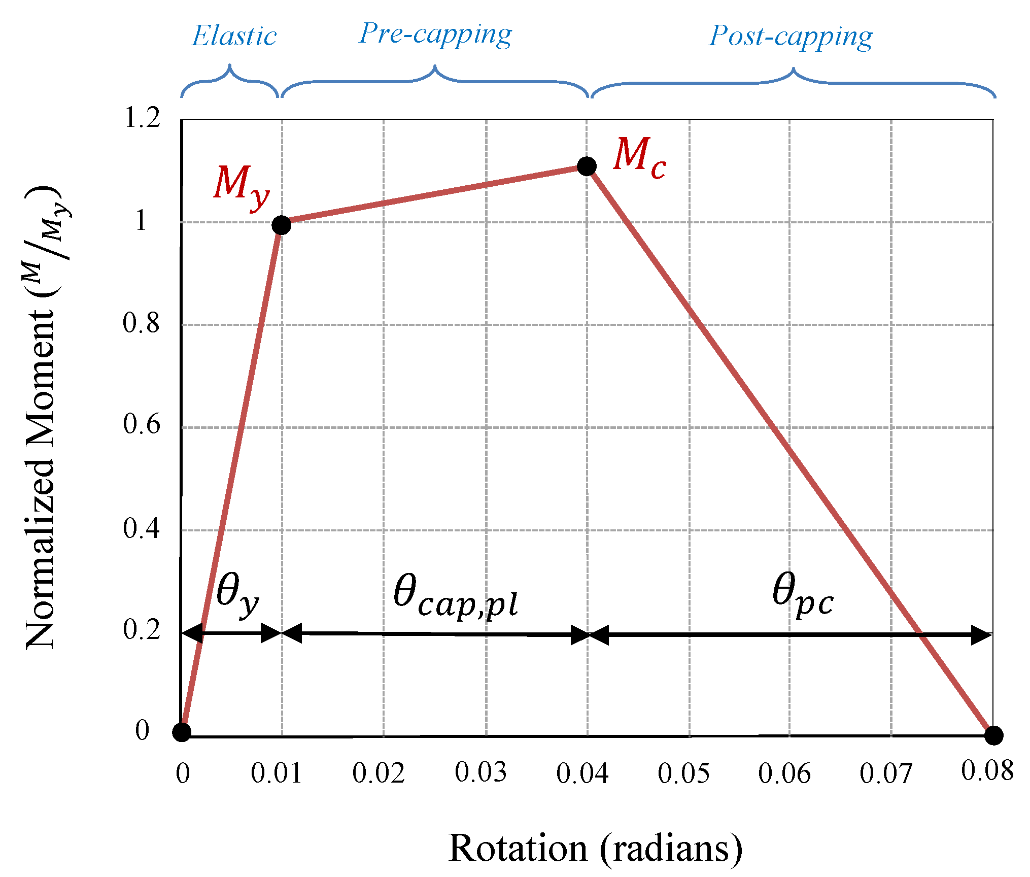
Among several nonlinear analysis techniques, the nonlinear static one (i.e., pushover) is used in this paper in order to determine the modeling parameters for each element of the frame. A lumped plasticity model, as opposed to the distributed one [18], is used for the beams and columns in which the element itself is assumed to be linear elastic, having two nonlinear plastic hinges at the ends [19]. The plastic hinge behavior is defined using the backbone curve of Ibarra et al. [20], as shown in Figure 1. To characterize a hinge element, the following parameters are required:

• $M_y$: Yield moment;
• ${\theta }_y$: Yield rotation;
• $M_c$: Ultimate moment;
• ${\theta }_{cap,pl}$: Plastic portion of the ultimate rotation;
• ${\theta }_c$: Ultimate rotation ($={\theta }_y+{\theta }_{cap,pl}$);
• ${\theta }_{pc}$: Post-peak rotation.

The relations to calculate the parameters in a backbone curve are elaborated in the following sections.

2.1. Modeling Parameters for RC Beams and FRP-Wrapped Columns

In order to determine the moment and rotation at the yield point (i.e., $M_y$ and ${\theta }_y$) for beams and columns, the equations suggested by Panagiotakos and Fardis [21], Biskinis and Fardis [22] are adopted. These relations were basically developed for non-retrofitted elements, and are summarized in Section 3.1. Therefore, they can be applied to the beams considered in the present study, because they are not to be retrofitted herein. As for the columns which are to be confined by FRP, it should be noted that the effect of FRP is revealed after expansion of the section under axial and flexural loading, and that the phenomenon occurs after yielding. Therefore, it seems to be reasonable to assume that by wrapping the columns with different numbers of FRP layers, the properties at the yield point (i.e., moment and rotation) remain unchanged as compared to the unconfined sections. Thus, the above-mentioned equations are employed to calculate $M_y$ and ${\theta }_y$ for FRP-confined columns, as well.

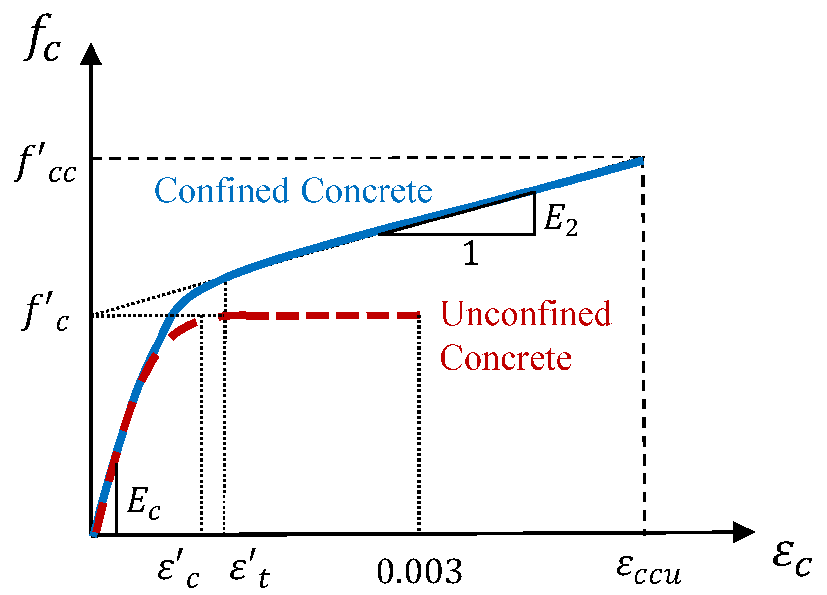
In order to identify the peak point of the backbone curve (i.e., $M_c$ and ${\theta }_c$), a moment–curvature analysis of the concrete section was performed. In the sectional analysis, which assumes plane sections remain plane, the axial load and the bending moment corresponding to a given neutral axis, and a section’s curvature are calculated [23]. A key part of this analysis is the stress–strain model employed for concrete. As for the columns wrapped with FRP, the uniaxial behavior of the confined part was considered to be based on the stress–strain model proposed by Lam and Teng [24], as demonstrated in Figure 2.

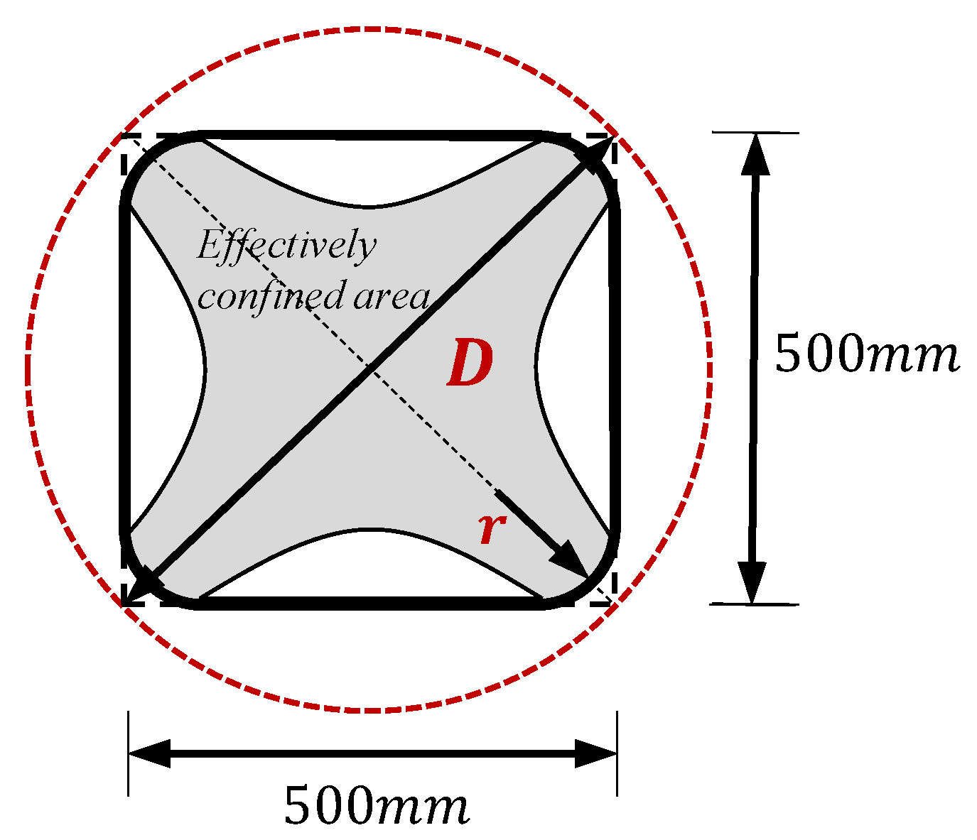
The mathematical expressions for the Lam and Teng [24] model are presented in Section 3.2. This material model can properly be used for concrete sections that are confined with different numbers of FRP layers (the same model is adopted by ACI 440 [25]). By putting the number of FRP layers equal to zero in the model of Lam and Teng [24], the stress–strain curve obtained by the model turns out to be that of unconfined concrete. A major advantage of this model lies in its applicability to rectangular sections while the majority of other models are limited to the circular sections. Among the available confinement models reported specifically for rectangular sections, the model of Lam and Teng [24] yields the best accuracy [26]. In rectangular sections, the effect of confinement is reduced as compared to the circular ones, and this is taken into account by defining the effectively confined area shown in Figure 3. Then, the rotation corresponding to a given sectional curvature is obtained by assuming a length for the plastic hinge, which is herein calculated based on the equation suggested by Paulay and Priestley [27], as presented in Section 3.2. As for beams, which are non-retrofitted herein, the ratio of $M_c/M_y$ was assumed to be equal to 1.13 [28]. In order to derive the last segment of the backbone curve, that is, the post peak rotation ${\theta }_{pc}$, the empirical equation proposed by Haselton and Deierlein [29] was used for beams and columns:

$${\theta }_{pc}=0.76{\left(0.031\right)}^{\nu }{\left(0.02+40{\rho }_{sh}\right)}^{1.02}\le 0.10,$$

(1)

where $\nu$ is the axial load ratio and ${\rho }_{sh}$ is the transverse reinforcement ratio.

In order to account for the effect of the FRP confinement of columns in Equation (1), the amount of transverse reinforcement appearing in the equation was calculated by adding the actual amount available in the section, plus a hypothetical amount drawn from equaling the confinement pressure induced by the FRP jacket and the pressure induced by equivalent steel hoops.

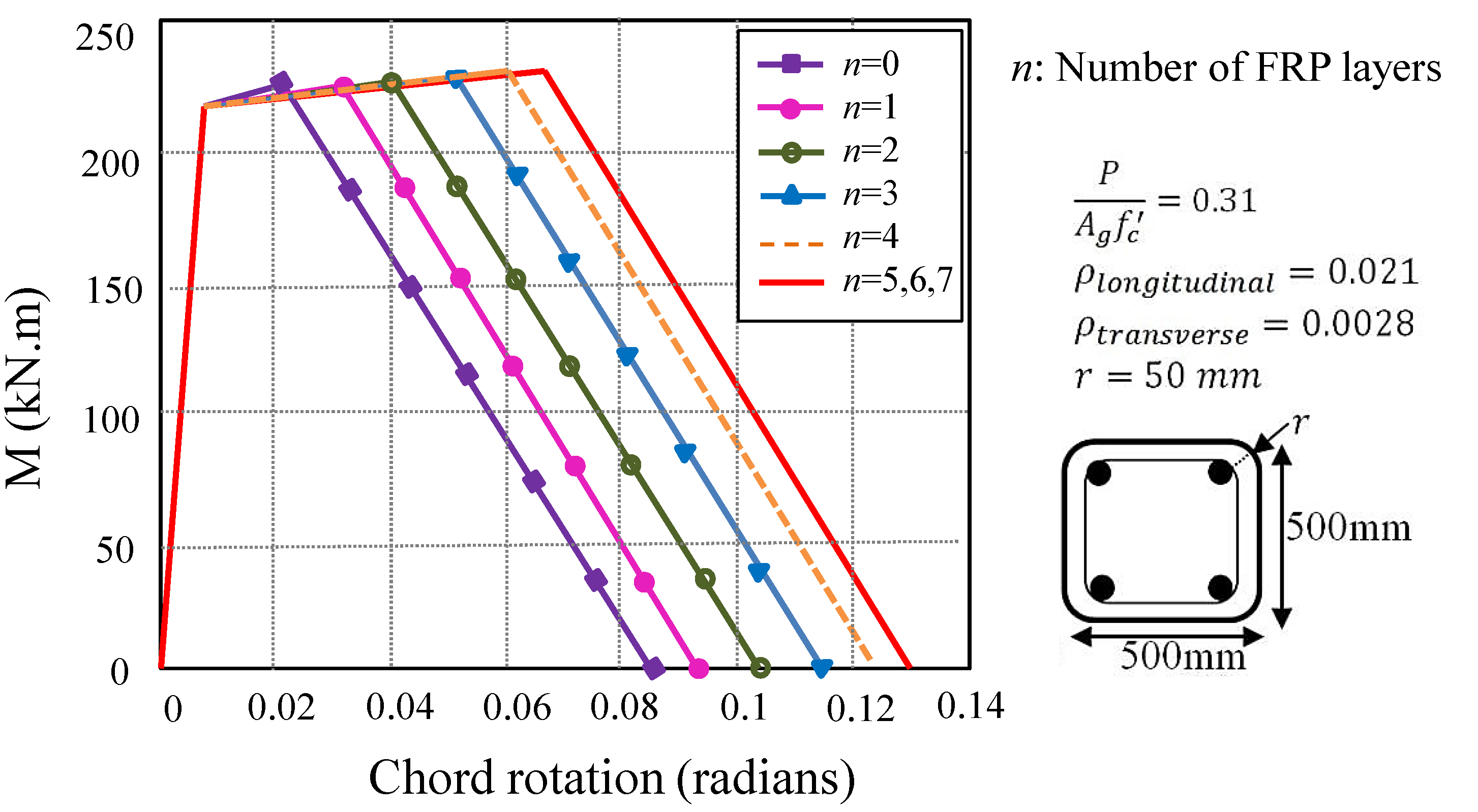
Finally, based on the above-mentioned relations, the backbone curves for the beams and retrofitted columns were established. As an illustrative example, Figure 4 shows the diagram of moment versus plastic hinge rotation for a sample column confined with different numbers of FRP layers under a given axial load ratio. It is evident from Figure 4 that the effect of confinement became negligible for the relatively large number of FRP plies.

2.2. Modeling Parameters for RC Beam–Column Joints

In order to model the beam–column joints in OpenSees software [30], a so-called Joint2D element was employed [31]. This model consisted of five springs: one central spring, and four others located at each side of the joint. The side springs represent the hinge elements of the surrounding beams and columns. They were connected to the central spring using multi-constraint objects to ensure same translational degrees of freedom as of the central one.

The central spring is responsible for the joint shear behavior, which in turn affects the whole response of the frame. Note that the effect of joint shear behavior is one of the prominent parts of the modeling procedure in the current study. For this purpose, extensive research has been conducted on different joint shear models which could be used for old, non-ductile, and non-code-conforming RC beam–column joints as reported in the literature. Some are: Theiss [32], Anderson et al. [33], Hassan and Moehle [34], Kim and LaFave [35], Lowes et al. [36], Montava et al. [37]. Some of the main characteristics of old and non-ductile joints are: (1) lack of sufficient shear reinforcement, and (2) inadequate lap splice length in the joint panel zone. Among all existing models, the one proposed by Anderson et al. [33] is used herein to define the shear behavior of beam–column joints in the RC frame.

3. Underpinning Theories for Moment–Rotation Relations: A Review

This section summarizes the relationships to calculate the moments and corresponding rotations for the yield point and the ultimate one.

3.1. Yield Point Relations ($M_y$ and ${\theta }_y$)

The yield moment is calculated as [21]:

$$\frac{M_y}{b{d}^3}={\varphi }_y\left\{E_c\frac{k_y^2}{2}\left(\frac{1+{\delta }^{\prime }}{2}-\frac{k_y}{3}\right)+\frac{E_s}{2}\left[\left(1-k_y\right)\rho +\left(k_y-{\delta }^{\prime }\right){\rho }^{\prime }+\frac{{\rho }_{sh}}{6}\left(1-{\delta }^{\prime }\right)\right]\left(1-{\delta }^{\prime }\right)\right\},$$

(2)

where ${\delta }^{\prime }=\frac{d^{\prime }}{d}$, and the neutral axis depth at yield level $k_y$ is determined by:

$$k_y={\left(n_s^2{A}^2+2n_{s}B\right)}^{1/2}-n_{s}A,$$

(3)

where $n_s=\frac{E_s}{E_c}$, and other terms are defined in the list of notations.

The values of A and B in Equation (3) depend on the potential failure modes:

• Mode 1: the yielding is a result of the yield of tension reinforcement; and
• Mode 2: the yield condition arises from the nonlinearity of the compression of concrete.

The relations are as follows:

$$A=\left\{\begin{array}{cc}\rho +{\rho }^{\prime }+{\rho }_{sh}+\frac{P}{bd{f}_y}& \mathrm{mode}1\\ \rho +{\rho }^{\prime }+{\rho }_{sh}-\frac{P}{1.8n_{s}bd{f}_c^{\prime }}& \mathrm{mode}2\end{array}\right.,$$

(4)

$$B=\left\{\begin{array}{cc}\rho +{\rho }^{\prime }{\delta }^{\prime }+0.5{\rho }_{sh}\left(1+{\delta }^{\prime }\right)+\frac{P}{bd{f}_y}& \mathrm{mode}1\\ \rho +{\rho }^{\prime }{\delta }^{\prime }+0.5{\rho }_{sh}\left(1+{\delta }^{\prime }\right)& \mathrm{mode}2\end{array}\right..$$

(5)

Next, the yield curvature is calculated as:

$${\varphi }_y=min\left\{\begin{array}{cc}{\varphi }_{y1}=\frac{f_y}{E_s\left(1-k_y\right)d}& \mathrm{mode}1\\ {\varphi }_{y2}=\frac{1.8f_c^{\prime }}{E_s{k}_{y}d}& \mathrm{mode}2\end{array}\right..$$

(6)

Finally, the rotation at yield condition is determined as [22]:

$${\theta }_y={\varphi }_y\frac{L_s+a_{v}z}{3}+0.0013\left(1+1.5\frac{h}{L_s}\right)+a_{sl}\frac{{\varphi }_y{d}_b{f}_y}{8\sqrt{f_c^{\prime }}}.$$

(7)

3.2. Ultimate Point Relations ($M_c$ and ${\theta }_{cap,pl}$)

A sectional analysis was conducted in order to calculate $M_c$ and ${\theta }_{cap,pl}$. To do so, the stress–strain, $f_c-{\epsilon }_c$ relationship proposed by Lam and Teng [24] for FRP-confined concrete square sections was employed with the following equations (Figure 2):

$$\begin{array}{c}\hfill f_c=\left\{\begin{array}{cc}{E}_c{\epsilon }_c-\frac{{\left(E_c-E_2\right)}^2}{4f_c^{\prime }}{\epsilon }_c^2& 0\le {\epsilon }_c\le {\epsilon }_t^{\prime }\\ f_c^{\prime }+E_2{\epsilon }_c& {\epsilon }_t^{\prime }\le {\epsilon }_c\le {\epsilon }_{ccu}\end{array}\right.,\end{array}$$

(8)

$$\begin{array}{c}\hfill \frac{f_{cc}^{\prime }}{f_c^{\prime }}=1+3.3{\kappa }_a\frac{f_l}{f_c^{\prime }},f_l=\frac{2E_{f}n{t}_f{\epsilon }_{fe}}{D},\end{array}$$

(9)

$$\begin{array}{c}\hfill {\epsilon }_{ccu}={\epsilon }_c^{\prime }\left(1.5+12{\kappa }_b\frac{f_l}{f_c^{\prime }}{\left(\frac{{\epsilon }_{fe}}{{\epsilon }_c^{\prime }}\right)}^{0.45}\right),\end{array}$$

(10)

$$\begin{array}{c}\hfill E_2=\frac{f_{cc}^{\prime }-f_c^{\prime }}{{\epsilon }_{ccu}},{\epsilon }_t^{\prime }=\frac{2f_c^{\prime }}{E_c-E_2},{\epsilon }_{fe}={\kappa }_{\epsilon }{\epsilon }_{fu},\end{array}$$

(11)

where ${\kappa }_a$ and ${\kappa }_b$ are the shape factors obtained based on arching action in the cross section (see Figure 3), and ${\kappa }_{\epsilon }$ was assumed to be 0.55. Other terms are defined in the list of notations. Furthermore, the following were used to determine the rotation:

$${\theta }_{cap,pl}=\left({\varphi }_u-{\varphi }_y\right)L_{pl};L_{pl}=0.08L_s+0.022f_y{d}_b.$$

(12)

4. Framework for Optimization of the Retrofit Plan

4.1. Formulation of the Objective Function

The objectives of the current optimization study were: (1) determining the number of FRP layers required to confine deficient columns of a reinforced concrete frame in order to enhance the seismic performance of the frame, (2) while keeping the consumption of FRP materials as minimal as possible. Therefore, the number of FRP layers needed for each column was assumed to be the “design variable” during the optimization process, which was herein taken between 0 to 8 layers. The lower limit of zero is to consider the case in which a column does not need any retrofit, while the upper bound is the limit beyond which adding extra FRP layers will no longer improve the backbone curve of the column.

For the purpose of optimization, the objective function was defined as Equations (14)–(17), where the cost of FRP retrofitting, which is considered linearly proportional to the number of FRP layers, is to be minimized under the condition of minimizing the COV for the plastic hinge rotation usage ratios of the columns. The column’s plastic hinge rotation usage ratio (denoted by $R_i$) is defined as the ratio of the existing plastic hinge rotation at each column end to the allowable plastic hinge rotation:

$$R_i=\frac{\mathrm{Existing} \mathrm{rotation} \mathrm{at} \mathrm{plastic} \mathrm{hinge}}{\mathrm{Life}-\mathrm{safety}-\mathrm{based} \mathrm{capacity} \mathrm{of} \mathrm{plastic} \mathrm{hinge} \mathrm{rotation}}.$$

(13)

The allowable plastic hinge rotation for a column is herein defined as 75% of ${\theta }_c$ according to ASCE/SEI-41-13 [38], and that corresponds to the life safety (LS) performance level for primary components. Minimizing the COV of $R_i$ values for all columns of the frame was performed with the aim of acquiring a uniform distribution for the plastic hinge rotation usage ratios around their mean value. Meanwhile, it is desirable that the $R_i$ values for all columns remain less than unity so as to meet the LS level of seismic performance (See Equation (3)). In order to achieve these conditions and avoid solving a multi-objective cost function, which is a time-consuming and computationally demanding task, one cost (or objective) function was employed, but the aforesaid conditions were considered as penalty terms introduced in the main cost function. In other words, the number of FRP layers was taken as the main part of the objective function whereas the COV of $R_i$ values was applied to the FRP cost as a penalty term such that in case of exceeding a specified limit, the cost function was increased considerably. The equation for the cost or objective function, F, is:

$$F=100\times \left(1+\frac{n_t}{n_{max}}\right)\times {\left(1+\sum _{i=1}^N{P}_i\right)}^2\times {\left(1+G\right)}^2,$$

(14)

where $n_t$ is the total number of FRP layers used and $n_{max}$ is the maximum number of FRP layers to be used (in this paper, eight layers per column). Other terms are as follows:

$$P_i=\left\{\begin{array}{cc}{R}_i-1& R_i>1\\ 0& R_i\le 1\end{array}\right.,$$

(15)

$$G=\frac{\mathrm{C}\mathrm{O}{\mathrm{V}}_{\mathrm{r}\mathrm{e}\mathrm{t}\mathrm{r}\mathrm{o}\mathrm{f}\mathrm{i}\mathrm{t}\mathrm{t}\mathrm{e}\mathrm{d}}}{\mathrm{C}\mathrm{O}{\mathrm{V}}_{\mathrm{o}\mathrm{r}\mathrm{i}\mathrm{g}\mathrm{i}\mathrm{n}\mathrm{a}\mathrm{l}}},$$

(16)

$$\mathrm{C}\mathrm{O}{\mathrm{V}}_{\mathrm{r}\mathrm{e}\mathrm{t}\mathrm{r}\mathrm{o}\mathrm{f}\mathrm{i}\mathrm{t}\mathrm{t}\mathrm{e}\mathrm{d}}=\frac{\sigma }{{\overline{R}}_l};\sigma ={\left(\frac{{\sum }_{i=1}^N{\left(R_i-{\overline{R}}_l\right)}^2}{N-1}\right)}^{1/2};{\overline{R}}_l=\frac{1}{N}\sum _{i=1}^N{R}_i,$$

(17)

where N is the number of columns’ plastic hinges (i.e., twice the number of columns in an RC frame), and $\mathrm{C}\mathrm{O}{\mathrm{V}}_{\mathrm{o}\mathrm{r}\mathrm{i}\mathrm{g}\mathrm{i}\mathrm{n}\mathrm{a}\mathrm{l}}$ is related to $R_i$ values before implementation of the seismic retrofitting, and is used as a scale factor in Equation (16).

For optimization of the objective function, two meta-heuristic algorithms were applied: (1) genetic algorithm (GA), and (2) particle swarm optimization (PSO). Both these techniques are implemented in MATLAB [39]. Two different optimization techniques were used in order to evaluate the sensitivity of the final solution to the employed algorithm.

4.2. Underpinning Theories for Genetic Algorithm with Application

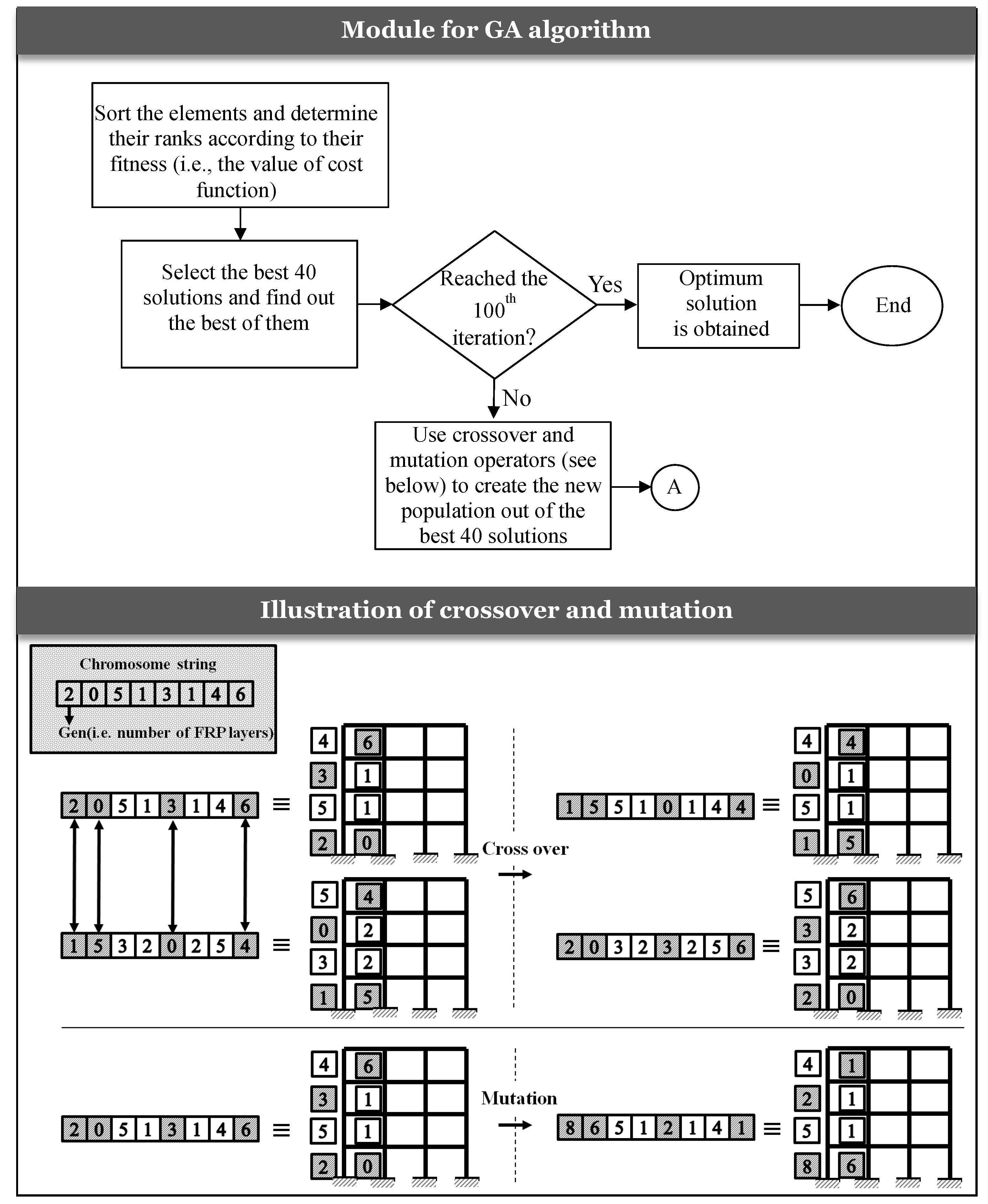
Genetic algorithms have their root in Darwin’s evolution of biological systems, and were originally developed by Holland et al. [40] in the 1960s–1970s. They are based on the law of nature—that is, fitter individuals have a greater chance of survival. The GA begins with a population containing several members. As for the problem at hand, each member represents a retrofit plan describing the number of FRP layers for each column in the considered frame. In the GA terminology, the number of FRP layers for each column is referred to as a “gene”, and a given retrofit plan is denoted by a “chromosome string”. Then, the procedure continues by applying several operators: (1) selection, (2) crossover, and (3) mutation to the initial population.

The selection operator, of Roulette wheel type [41], was employed to derive two other populations out of the initial population: (1) the parent population which is used to produce the “children”, population by means of the crossover operator, and (2) the population is subjected to a mutation process. The crossover is uniform [41] and combines a pair of members from the parent population by swapping a set of randomly chosen gens of one member for the corresponding gens in the other member, so as to produce two new members. This herein means for some chosen columns, the numbers of FRP layers are interchanged between two possible retrofit plans, as shown in Figure 5. The mutation deals with a member (i.e., a chromosome) of a population to replace some gens of that member with new gens while keeping the rest of gens unchanged. In the context of the current application, this implies that for a considered retrofit scheme, the numbers of FRP layers for some randomly selected columns are altered to other values randomly taken from the possible range of values except for the current value (see Figure 5).

For each member of the populations generated above, the cost function is evaluated and the members are sorted based on the lowest values of the cost function. Finally, the best fitted members are selected to form the new population for the next iteration. The process terminates when it reaches the predefined maximum number of iterations. The initial population was assumed to have 40 members, and the maximum number of iterations was set to 100. The optimal solution is the most fitted member, which provides the lowest cost function value. Figure 5 demonstrates a flowchart summarizing the above-mentioned process.

Subsequently, the genetic algorithm utilizes a strategy based on the survival of the fittest member to produce the next generation, which helps the procedure gradually yield the optimal solution. Furthermore, the application of the mutation rule has made the algorithm capable of finding the solutions which are far from the initial point at which the algorithm has started exploration, i.e., helps the algorithm get out of the local optimum points.

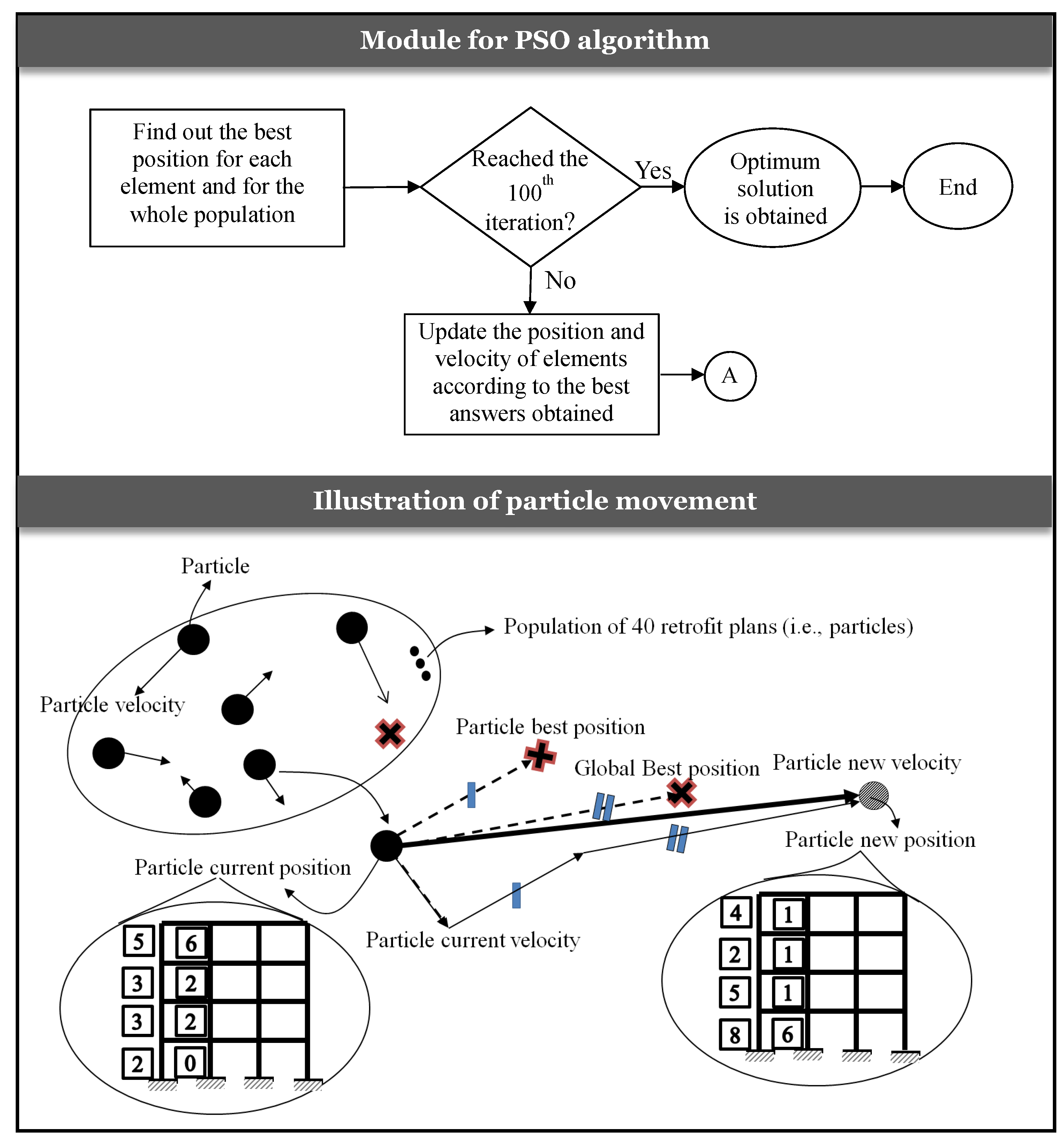
4.3. Underpinning Theories for Particle Swarm Optimization with Application

The particle swarm optimization (PSO) [42] algorithm begins with a population (i.e., swarm) of members (i.e., particles) which are considered as candidate solutions to the problem. The idea is to move particles in the response space such that better positions are obtained in order to yield lower values of the cost function. Each particle’s position is defined by the coordinates in the n-dimensional space, and its movement is characterized by an increment (i.e., velocity) imposed to each coordinate.

In the context of the current example, an assumed retrofit pattern of the considered frame is treated as a particle whose position has n coordinates, where each coordinate is referred to as the number of FRP plies for a particular column (n is the number of columns in the frame). At each iteration, the so-called velocity vector (whose coordinates are the imposed increments corresponding to the coordinates of the particle’s position), is employed to move the particles to new positions, and the cost function is evaluated. Next, for each particle, and during the successive iterations, the minimum value of the cost function is identified. This means identifying the best position that the considered particle has ever experienced (i.e., the particle’s best position). Besides, the absolute minimum value of the cost function for all the particles is determined, and the corresponding particle’s position is called the global best position.

Both global and particle best positions are employed to define the velocity needed to move each particle in the next iteration. In other words, the velocity for a particle in each iteration depends on three terms: (1) the current position of that particle, (2) the best position ever experienced by that particle, and (3) the best position ever found by the entire population (i.e., the global best position).

Thereby, the new velocity of each particle, $v_i^{t+1}$, is derived by adding the current velocity of that particle, $v_i^t$, to the vector connecting the current position of the particle, $x_i^t$, to the particle’s best position, $x_i^{*}$, and the vector connecting the current position to the global best position, $g^{*}$, which are multiplied by some factors.

$$v_i^{t+1}=v_i^t+{\alpha }_1{ϵ}_1\odot \left[g^{*}-x_i^t\right]+{\alpha }_2{ϵ}_2\odot \left[x_i^{*}-x_i^t\right],$$

(18)

where ${ϵ}_1$ and ${ϵ}_2$ are two random vectors within [0, 1]; ⊙ presents the Hadamard product of two matrices; and ${\alpha }_1$ and ${\alpha }_2$ are the learning parameters or acceleration constants (typically are taken as 2) [43].

The new velocity obtained in this way is then added to the current position of the particle, $x_i^t$, to achieve the new position in the subsequent iteration (assuming that the initial velocity of a particle is zero):

$$x_i^{t+1}=x_i^t+v_i^{t+1}.$$

(19)

Figure 6 illustrates a flowchart for implementation of the PSO within the current application. The aforementioned procedure of moving the particles towards the best positions ever found in the response space helps the algorithm gradually approach the optimum solution. Here, the initial population for the PSO algorithm was assumed to be similar to the one in GA, and contained 40 particles randomly generated with different positions. In the first iteration, each particle’s velocity vector was assumed to be zero, and the total number of iterations was taken as 100.

5. Illustrative Example of an RC Frame Structure

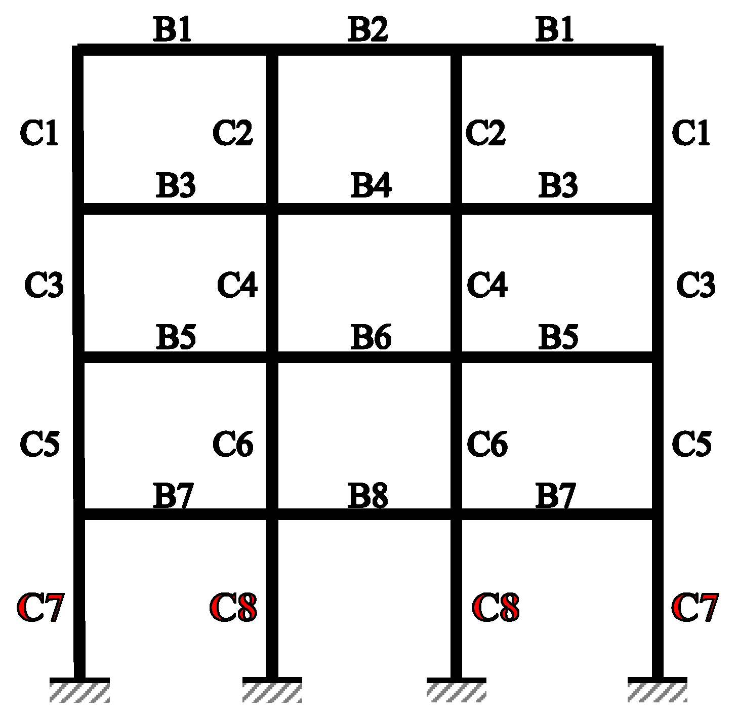
In order to elaborate on the methodology of the retrofit scheme design using the explained optimization procedure, a four-story three-bay reinforced concrete frame was adopted. The structural design and dynamic response can be found in Liel and Deierlein [28], Figure 7, and the geometry of the columns and beams is reported in

Table 1. Column dimensions and reinforcement for the case study frame; ${\rho }_{tot}$ and ${\rho }_{sh}$ are longitudinal and transverse reinforcement ratio, respectively.

ID	B (mm)	h (mm)	L (mm)	${\mathit{\rho }}_{\mathit{tot}}$	${\mathit{\rho }}_{\mathit{sh}}$	s (mm)
C1	500	500	4000	0.021	0.0022	250
C2	500	500	4000	0.012	0.0015	250
C3	500	500	4000	0.021	0.0022	250
C4	500	500	4000	0.019	0.0015	250
C5	500	500	4000	0.021	0.0022	250
C6	500	500	4000	0.021	0.0028	250
C7	500	500	4600	0.026	0.0039	250
C8	500	500	4600	0.021	0.0028	250

and

Table 2. Beam dimensions and reinforcement for the case study frame; $\rho$ and ${\rho }^{\prime }$ are top and bottom longitudinal reinforcement ratios, respectively; and ${\rho }_{sh}$ is the transverse reinforcement ratio.

ID	B (mm)	h (mm)	L (mm)	$\mathit{\rho }$	${\mathit{\rho }}^{\prime }$	${\mathit{\rho }}_{\mathit{sh}}$	s (mm)
B1	500	500	8000	0.0125	0.0193	0.0055	230
B2	500	500	8000	0.0125	0.0193	0.0044	230
B3	500	500	8000	0.0115	0.0205	0.0044	230
B4	500	500	8000	0.0115	0.0205	0.0044	230
B5	500	650	8000	0.0065	0.0135	0.0028	300
B6	500	650	8000	0.0065	0.0135	0.0028	300
B7	500	650	8000	0.0073	0.0143	0.0028	300
B8	500	650	8000	0.0073	0.0143	0.0028	300

, respectively. The compressive strength of the concrete, and the yield stress of the steel reinforcements were considered as 27.5 and 413 MPa, respectively. The total applied gravity load (including the dead and live loads) was 50 kN/m. This frame was categorized as a non-ductile one, in which there are some deficiencies regarding code ductility requirements. It was also considered to be located in an area with high seismic demand. The frame was modeled in the OpenSees environment [30] and analyzed using a static nonlinear pushover procedure.

The lateral load pattern defined in pushover analysis is considered proportional to the frame’s first mode shape. In order to take the P-delta effect into account, an additional truss element was inserted in one side of the frame which is connected to the main frame by flexural hinges. The problem was to find the optimal scheme for FRP wrapping of the columns in the considered frame. In the optimization process, both the GA and PSO algorithms with the population of 40 and 100 iterations were used to minimize the objective function. The characteristics of the FRP layers used to retrofit the frame are listed in

Table 3. Characteristics of FRP layers used for retrofit.

Thickness, $t_f$ (mm)	0.33
Ultimate tensile strength, $f_{fu}^{*}$ (GPa)	3.79
Rupture strain, ${\epsilon }_{fu}^{*}$ (mm/mm)	0.0167
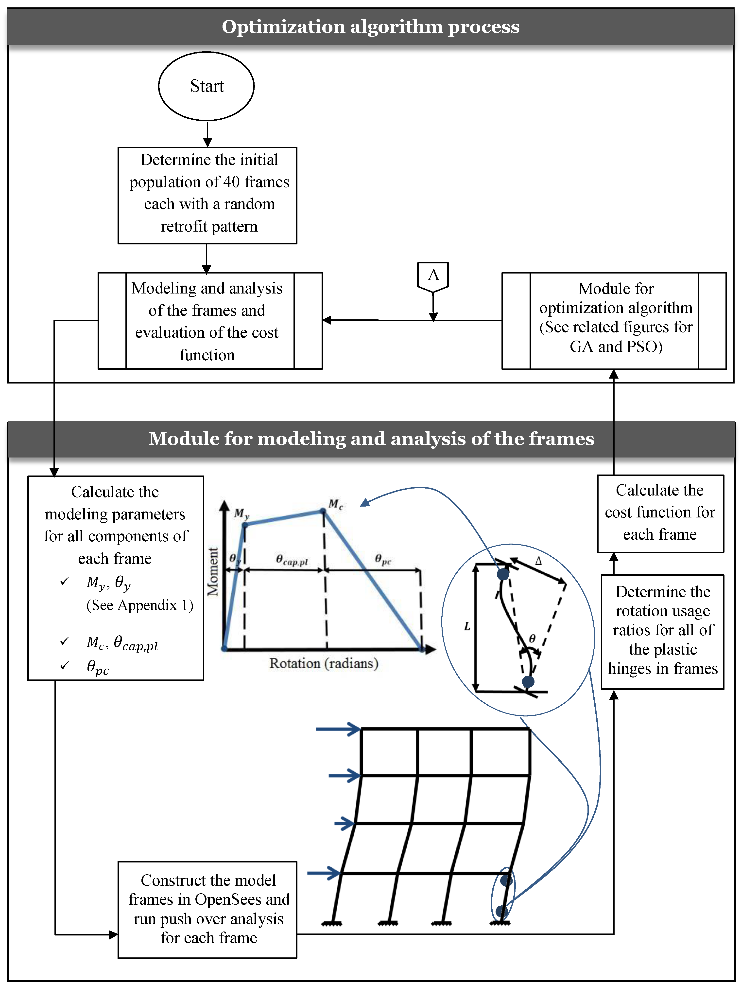
Elastic modulus, $E_f$ (GPa)	227.53

. The step-by-step procedure of optimization is illustrated in Figure 8 (with cross reference to Figure 5 and Figure 6), and can be summarized as follows.

• The first step in the optimization process is the initialization, in which an initial population of members (i.e., candidate solutions) is created. For each individual member of the population, a value is assigned to each design variable, which herein is the number of FRP layers for each column of the frame.
• Next, the frame components are modeled according to the initial amount of FRP layers at each column and the whole frame model is constructed in OpenSees program. The pushover analysis is performed, and the results of the target displacement are sent back to the optimization process. Subsequently, the cost function is evaluated for each member of the population.
• After calculation of the initial cost functions, the population members are sorted according to their fitness values, and the best results are drawn consequently.
• To this point, both GA and PSO optimization algorithms worked the same. The difference arises when the next generation is to be produced. In the genetic algorithm, the next generation is created by applying crossover and mutation operators to the initial population; whereas in PSO, it is produced by imposing a velocity to each particle in order to move it to a new position.
• After the next generation is created, the steps 2 to 5 are repeated for the next iteration, while the best answer of each iteration is being recorded. This procedure continues until the number of iterations reaches the maximum. At each iteration, and for each member of the populations, a nonlinear static pushover analysis was carried out.

As a final outcome, the optimum FRP retrofit scheme for the considered RC frame covers only the columns of the first floor, while the other columns remain as they are. The optimum retrofit plan consists of three layers of FRP wraps for the external columns, and six FRP layers for the interior columns of the first floor.

6. Results and Discussion

6.1. Convergence Performance of the Optimization Algorithms

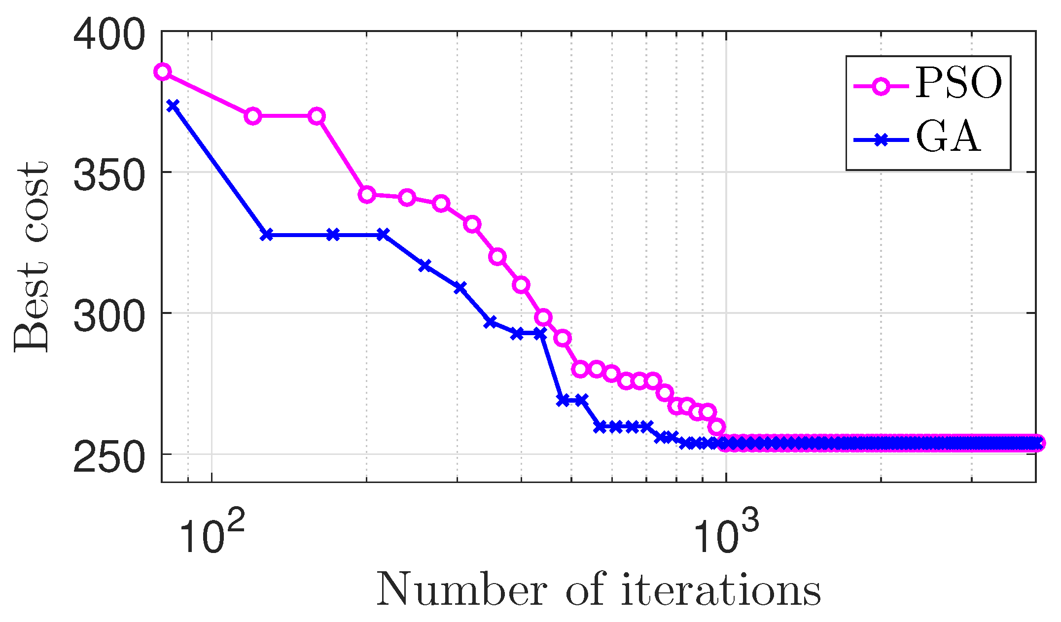
The two optimization algorithms (i.e., GA and PSO) provided the same solutions for the frame retrofit scheme. In both algorithms, the columns of the first floor are retrofitted with three and six layers of FRP on external and internal sides, respectively. Figure 9 illustrates the partial advantage of GA compared to the PSO. The GA reached the optimal solution after 832 iterations, in comparison to PSO, which converged after 1000 iterations.

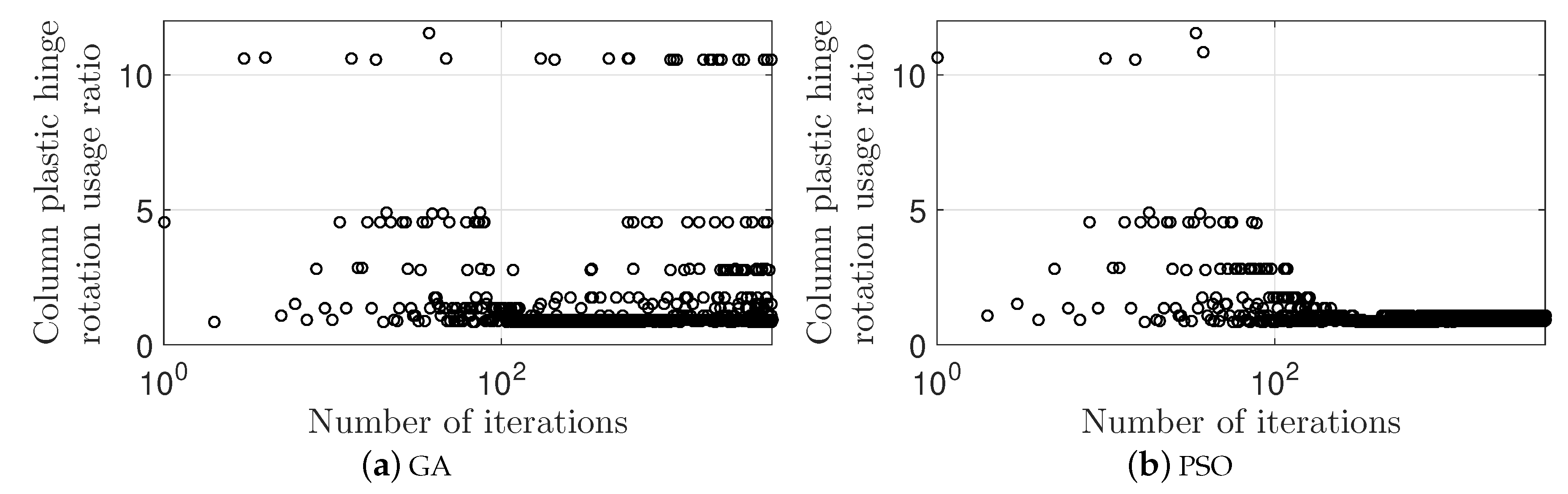
Figure 10 shows the maximum values for the usage ratios of the plastic hinge rotation capacity in the columns of the first floor in various iterations of GA and PSO. It is evident that PSO had less dispersion. The GA algorithm included some fluctuations even at higher iterations. This is because the PSO algorithm uses a highly efficient exploration method, as it was capable of converging to the optimum answer without deviating in higher iterations. Conversely, it is observed that during the GA process, even in higher iterations, there were still some answers found which had significant distance from the final optimum response of the algorithm. However, we emphasize that a general comparison between the performances of PSO and GA is beyond the scope of this paper, and the results presented herein are specific to the problem at hand.

6.2. Performance Evaluation of Retrofit Schemes

As stated earlier, in the optimum retrofit scheme proposed herein, only columns of the first floor are to be retrofitted. The numbers of FRP wraps are non-uniform among the columns, such that three and six layers are used for external and internal columns, respectively. This gives a total of 18 plies of FRP for all the columns of the first floor. Next, this optimal retrofit plan was compared with other retrofit schemes in which all columns of the first floor are uniformly wrapped with a certain number of FRP plies—that is, 1, 2, 3, 4, 5, or 6 plies per column (or alternatively 4, 8, 12, 16, 20, or 24 layers for all columns of the first floor).

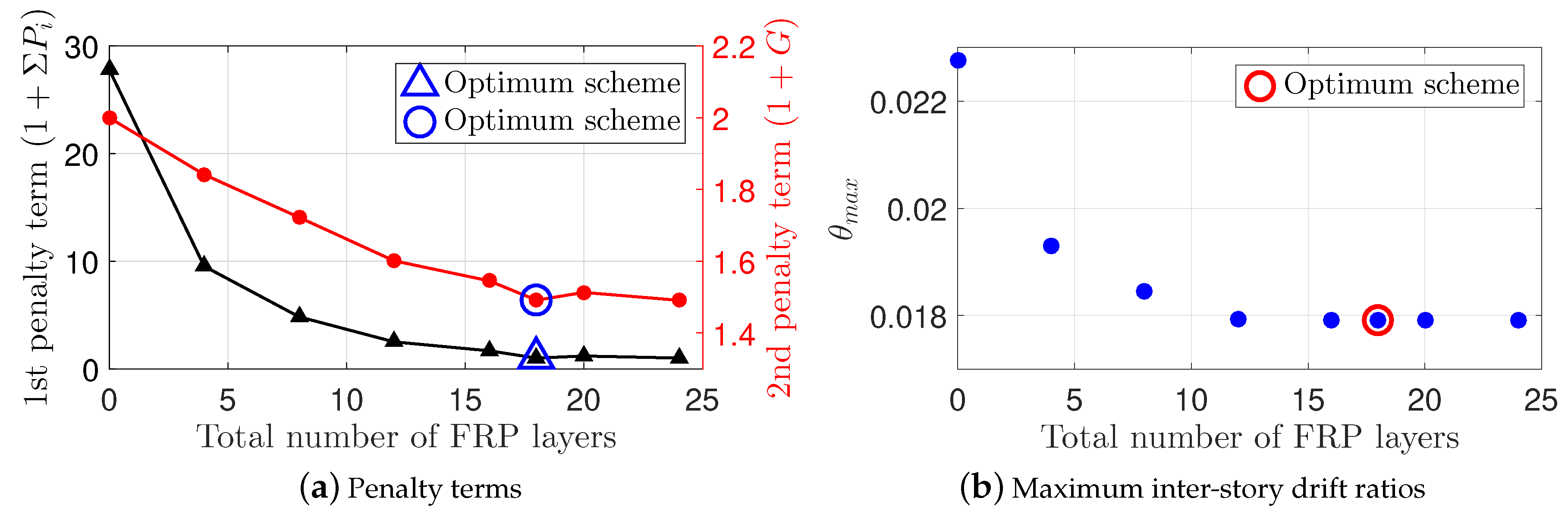
This comparison was conducted based on several measures. First, the variations of the penalty terms appeared in the objective function (i.e., Equation (14)) were evaluated in terms of different numbers of FRP plies used in the columns of the first floor, as illustrated in Figure 11a. The first penalty term in Equation (14), that is, ${\left(1+{\sum }_{i=1}^N{P}_i\right)}^2$, assured that the retrofit schemes which possess the columns with plastic hinge rotation usage ratio (i.e., $R_i$) greater than 1 were not considered as optimum solutions. Besides, the second penalty term, that is, $\left(1+G\right)$, was aimed at providing a uniform distribution of the column hinge rotation usage ratios among all columns of the frame. From Figure 11a, it is evident that for the proposed optimal retrofit scheme, both of the penalty terms reached their minimum values simultaneously.

As an optimization algorithm, this result is important in the sense that it is achieved by only one objective function (i.e., Equation (14)), instead of introducing several parallel objective functions to be optimized simultaneously. According to Figure 11a, at the optimum solution, the COV for $R_i$ values was reduced to almost half of that in the non-retrofitted frame.

The reason behind the non-uniform wrapping scheme for optimal retrofit rather than a uniform model can be attributed to the smaller plastic hinge rotation for the external columns at the target displacement compared to the internal columns. Therefore, the uniform distribution of $R_i$ values among the columns of the first floor can be achieved by providing fewer FRP plies for external columns compared to the internal ones, as is the case for the optimum retrofit plan proposed herein.

Figure 11b depicts the maximum inter-story drift ratios for different retrofit schemes. In all retrofit plans, except for the optimum scheme, the FRP wrapping was uniform for the first floor columns, meaning that both external and internal columns were wrapped with the same numbers of FRP plies. Figure 11b shows that the maximum inter-story drift ratio stopped decreasing when the number of FRP plies reached more than about three per column (or 12 plies for all four columns) of the first floor. In other words, if the amount of FRP used varies in the range of three to six plies per column, which also includes the optimum retrofit scheme, the maximum inter-story drift ratios would be practically unchanged.

6.3. Impact of FRP Retrofitting on Structural Response

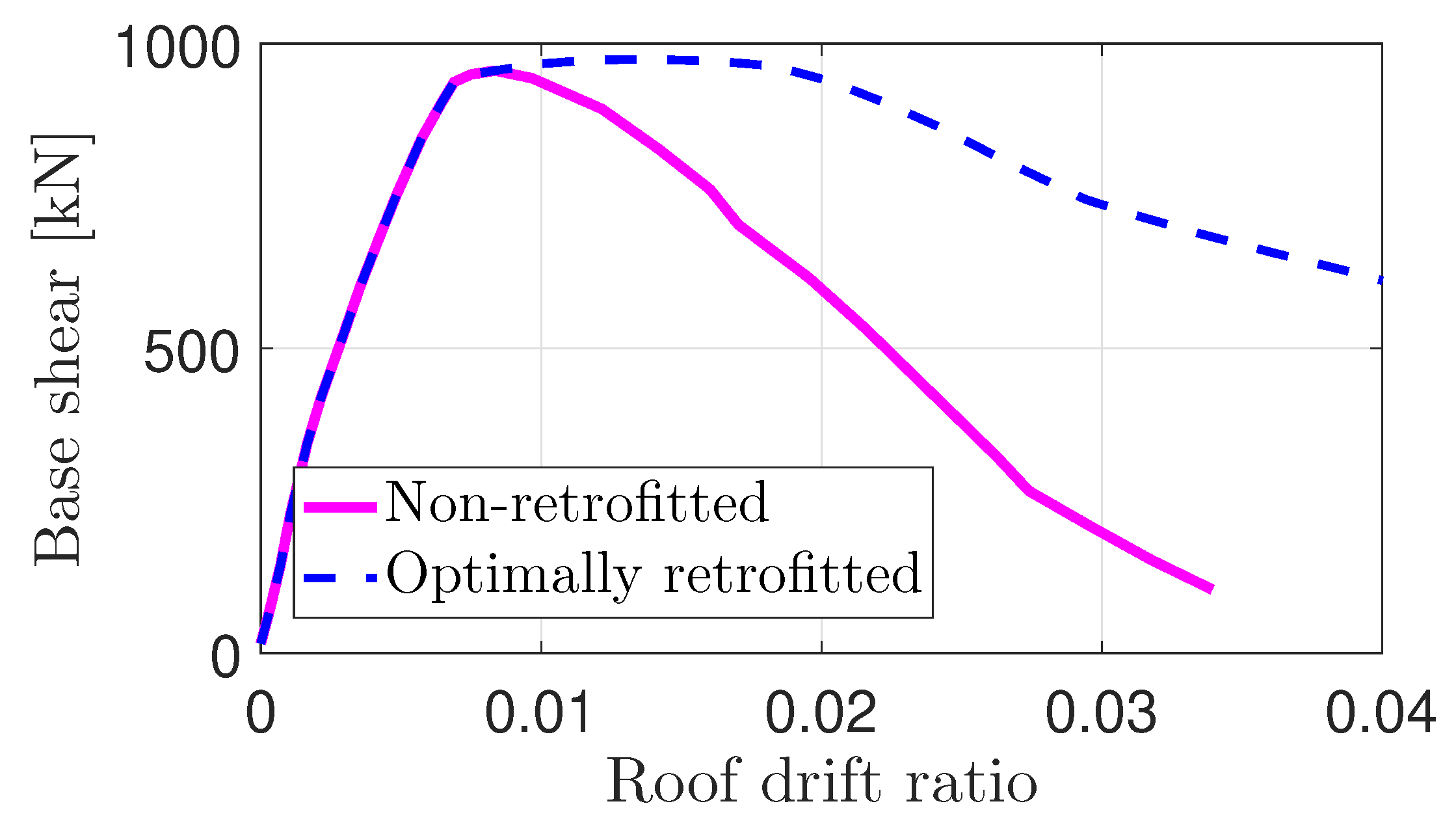
As explained earlier, the FRP confinement of concrete columns enhances the plastic hinge rotation capacity of the columns, and consequently improves the global response of the retrofitted frame. This result can be drawn from the pushover curve more precisely, Figure 12. It can be perceived that the lateral load carrying capacity—and more importantly, ductility—were enhanced after the columns were confined with FRP layers. This conclusion is obtained from the fact that the maximum roof displacement undergone by the retrofitted frame before the significant drop of the lateral strength was increased noticeably in comparison with the non-retrofitted frame. In addition, the maximum base shear experienced by the retrofitted frame was higher than that in the non-retrofitted frame.

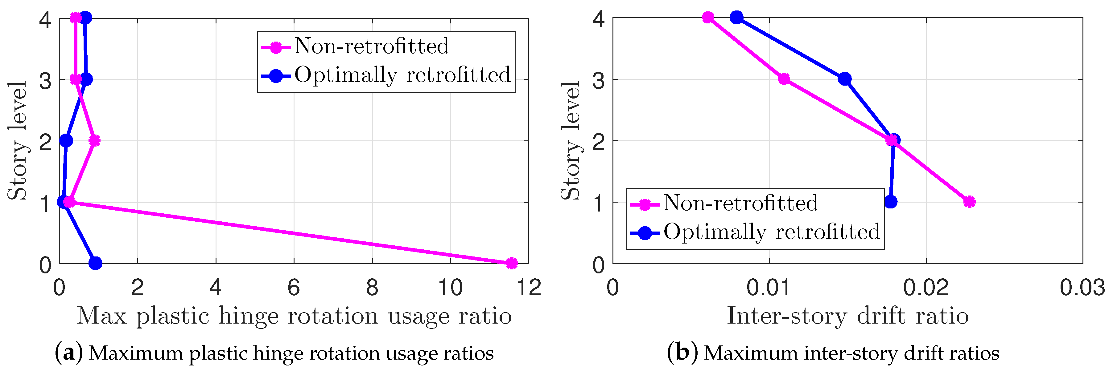
For the sake of comparison, the maximum values of the column plastic hinge rotation usage ratios (i.e., $R_i$) at different floor levels are demonstrated in Figure 13a. $R_i$ for the first story of the non-retrofitted frame went far beyond unity, indicating that the original non-retrofitted frame failed to meet the life safety performance level, and thereby it was in need of seismic retrofitting. According to Figure 13a, once the frame was retrofitted, the value of $R_i$ in the first floor decreased significantly to a value less than unity, as desired. This also yielded a more uniform distribution for the values of $R_i$ along the height of the retrofitted frame as opposed to the non-retrofitted case. This result is expected, since one of the optimization objectives was to reduce variations of the $R_i$ values in the frame.

On the other hand, the variations of the inter-story drift ratios along height of the frame were examined for the optimally retrofitted frame versus the non-retrofitted frame, as illustrated in Figure 13b. The initial frame experienced a maximum inter-story drift ratio of 2.3% in the first story, which is beyond the 2% limit of the life safety performance level according to ATC-40 [44]. This is in contrast to the retrofitted frame, in which the maximum inter-story drift ratio was about 1.8% (i.e., less than 2%). Besides, the optimally retrofitted frame developed a more uniform distribution of the inter-story drift ratios along the frame height as compared to the non-retrofitted case.

6.4. Fragility Assessment of FRP Retrofitted Frames

In order to further validate the result of the optimization process, a fragility assessment was performed [45]. A fragility curve represents the probability of exceeding a given damage state (e.g., life safety performance level) in terms of an earthquake-related demand indicator (e.g., peak ground acceleration, PGA; first-mode spectral acceleration, $S_a\left(T_1\right)$) [46]. There are various methods to develop seismic fragility curves for framed structures [47,48,49]. In this study, the fragility curves were derived using SPO2IDA [50], which is a tool to derive the 16%, 50%, and 84% summarized IDA curves based on the pushover analysis results. 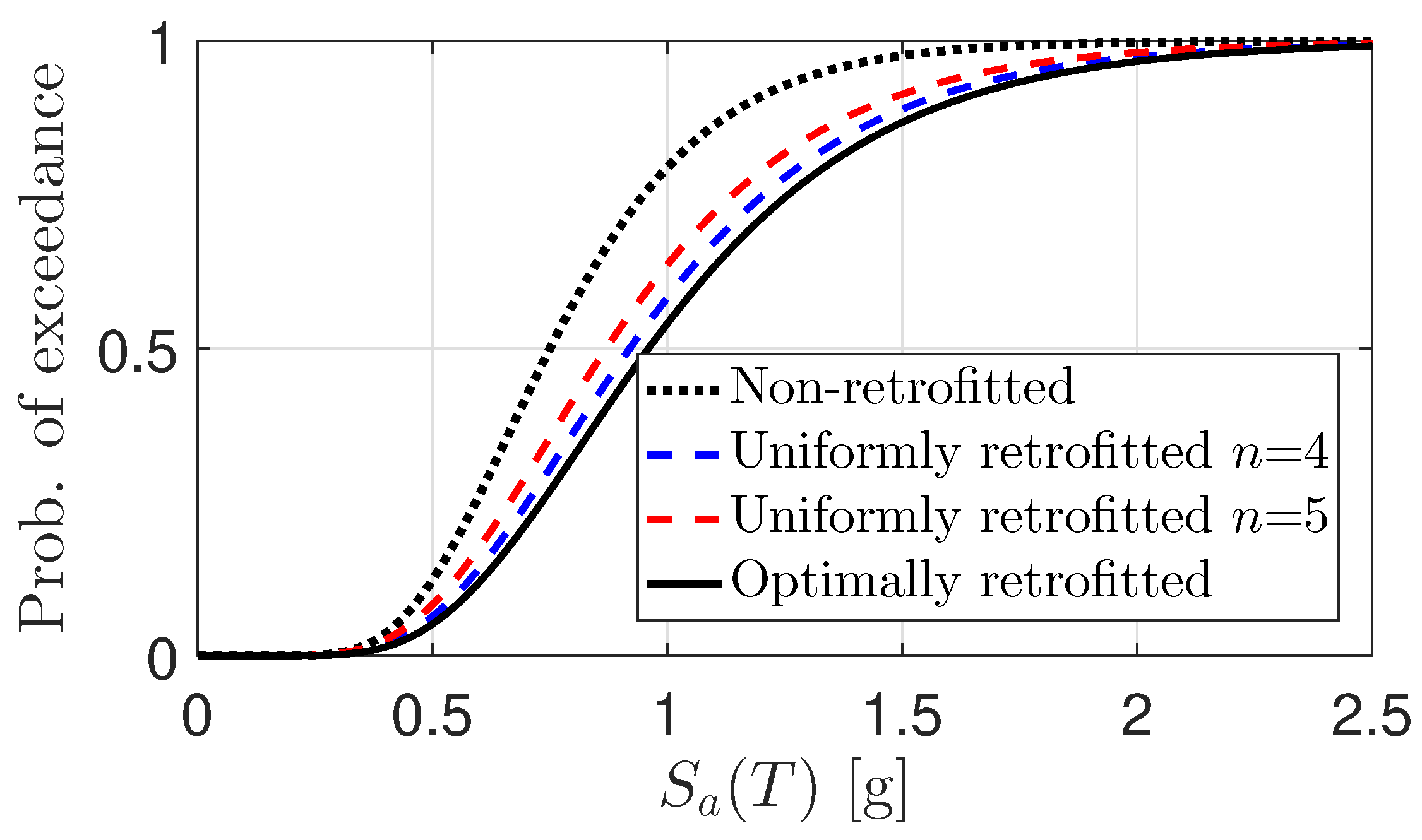Figure 14 shows the fragility curves for life safety performance level for the frames in which the first floor columns were all retrofitted uniformly with a certain number of FRP layers. To clarify, for instance n = 4 means that all the columns of the first floor are confined with four layers of FRP sheets in their plastic hinge zones. This figure also shows the non-uniform FRP retrofit plan with the optimal scheme obtained from the meta-heuristic algorithm. The spectral acceleration corresponding to the median value (i.e., the probability of exceeding 50% damage) for the fragility curve of the optimum retrofit scheme was larger than others. A fragility curve with a higher median value indicates a better performance. Thus, it is concluded that among all fragility curves for the retrofit schemes, the proposed optimum scheme, which has the lowest consumption of the FRP layers, had the highest performance level. Finally, the original non-retrofitted frame always had a higher probability of exceedance than the retrofitted ones.

7. Conclusions

In this paper, a systematic approach is developed to propose an optimal retrofit plan for reinforced concrete framed structures. The objective was to confine the columns by different numbers of FRP wraps along their plastic hinges. The criterion to formulate the optimization problem is based on providing a uniform distribution of the plastic hinge rotation usage ratios, denoted by $R_i$, among all columns, while minimizing the consumption of the FRP materials. The $R_i$ is herein defined as the ratio of the plastic hinge rotation experienced by a column to its plastic hinge rotation capacity corresponding to the life safety seismic performance level. Besides, the value of $R_i$ for each column should be less than unity to meet the life safety performance level criteria. These criteria were introduced into a single objective function as a couple of penalty terms.

In order to evaluate the capacity of the plastic hinge rotation, the effect of FRP confinement on the moment–curvature backbone curve of the column was quantified by a sectional analysis along with some empirical relations available in the literature. The values of $R_i$ obtained from pushover analyses of the frame were fed, at each iteration, into the objective function, which was then optimized by means of two different meta-heuristic algorithms (i.e., genetic algorithm and particle swarm optimization). The developed procedure was applied to a four-story three-bay RC frame suffering from a lack of ductility. The following major conclusions can be drawn:

• The optimum retrofit scheme obtained from optimization by GA was similar to the one resulting from PSO for the case study structure, in spite of the differences between the two meta-heuristic algorithms in terms of convergence speed and the fluctuations around the optimal solution. This suggests that the final optimal solution is independent of the optimization algorithm.
• In the optimal plan for seismic retrofitting of the sample frame, only the first story columns are in need of wrapping with FRP layers, while the other columns remain non-retrofitted. Furthermore, we concluded that the number of FRP layers needed for the external columns is less than for the internal ones (i.e., three vs. six FRP plies in the case study frame). The reason for this is that the plastic hinge rotation of an external column is different from that of an internal column when the frame is subjected to a target lateral displacement. Subsequently, different levels of FRP confinement are needed for external and internal columns to obtain similar $R_i$ values for all columns.
• The optimal retrofit scheme, in which only the first story columns are confined by different numbers of FRP layers, improved the pushover/capacity curve of the case study frame in terms of both the maximum base shear and the ultimate drift ratio at the roof level. Besides, the $R_i$ values of the first story columns dropped from large values in the original frame to less than unity in the optimally retrofitted frame, as required to satisfy the life safety performance level. Also, the maximum inter-story drift ratio of the first story, which was about 2.3% in the original frame, decreased to about 1.8% in the optimally retrofitted frame. It is concluded that the optimal retrofit scheme proposed herein developed much more uniform distributions of both plastic hinge rotation usage ratios and the inter-story drift ratios along the building height as opposed to the non-retrofitted frame.
• The fragility curve of the case study frame retrofitted based on the proposed optimal scheme was derived and compared with other retrofit plans, in which the first story columns are confined with a uniform number of FRP layers. Results show that the fragility curve of the optimal retrofit plan outperformed other fragility curves, which correspond to the similar amounts of FRP material consumption.

The current research indicates the efficiency of the proposed method in optimizing the retrofit plan for a reinforced concrete frame structure, in terms of the FRP confinement of columns. However, some of the results explained above may be specific to the frame under study. Thus, future investigation can be directed on investigations for a wide range of “RC frame classes” with different geometrical and mechanical characteristics. This means that a group of frames with different numbers of stories and bays should be retrofitted using the proposed algorithm. The effects of 2D vs. 3D framed structures, ductility, and design uncertainty should also be investigated. An effective optimization solver will then be required for this large-scale simulation-based database.