1. Introduction
The amount of global energy consumption in buildings represents 4.4% of heating and cooling demands. It is expected to increase to 35% in 2050, and 61% in 2100, due to the combination of both global warming and the inclusion of air conditioning in the market [
1]. Cooling demand represents 10% of the total energy demand pertaining to the Mediterranean region [
2]. In Spain and Italy, the cooling demand increased by 30% since 2005 to 2009 [
3]. Because of this occurrence, it is necessary to adopt energy efficiency measures that counteract the effects of inadequate architectural design.
The residential sector is responsible for 25.4% of the final energy consumption in the Eurostat Statistics (EU28) [
4]. However, it represents 63% of the potential building energy savings that can be obtained around 2050 [
5]. Less than 20% of residential buildings in Europe decide to overheat buildings instead of assuming cooling costs [
6]. Therefore, very few cities in Spain would need to consume energy in air conditioning under good conditions of thermal inertia and solar protection [
7,
8].
The use of air conditioning in Spain is very low. According to the latest official report on heating and air conditioning in the homes of the National Institute of Statistics of Spain (INE, 2009), 35.5% of Spanish dwellings are provided with air conditioning and 70.3% are provided with heating systems. When considering the hottest climate zones (i.e., those that are identified as being hot or very hot), 43.1% of dwellings are provided with a heating system and 57.4% of them include air conditioning. Regarding moderate climate zones (C4), 79.7% of the houses have a heating system whereas 58% of them have air conditioning. With respect to cold climate zones (D3), 90.4% are heated and 43.5% are cooled, whereas in very cold climate zones (E1), 90.8% are heated and only 3.3% are cooled [
9].
Currently, the American Institute of Architects encourages designers to use energy simulation [
10]. Building designers perform a fundamental role in achieving better energy efficiency systems in their projects [
11]. The most influential decisions in energy optimization are made at the early stages of the design process [
12,
13,
14]. Usually, designers apply those analyses too late [
15].
Thermal models are developed from details to the whole, as opposed to the architectural design [
16]. This is one of the reasons why existing energy simulation tools do not meet the needs of architects [
17,
18]. In addition, they are too complex [
19]. Due to this fact, architects do not consider energy modeling as an issue that is their responsibility [
20]. Therefore, the use of simulation tools remains deficient [
21].
Although the existing research works focus on the impact of design variables on energy objectives, most studies ignore the urban context as a key design variable. However, some research works analyzed the influence of the urban context on the energy efficiency of buildings. For example, the influence of the height to width ratio of buildings (H/W) or that of urban canyons on the energy efficiency of buildings are often considered [
22,
23,
24,
25,
26,
27,
28,
29,
30]. The increment in ambient air temperatures in cities increases the thermal stress in the built environment as well as the cooling demands [
31,
32,
33].
The storage of solar energy through irradiation in buildings, the thermophysical properties of materials, and the urban context are controllable factors that directly influence the increment in temperatures [
34]. Therefore, strategies for reducing the urban heat island effect are based on considering the thermal and radioactive properties, such as the albedo, emissivity, and roughness of urban materials, among other properties [
35,
36,
37]. In Spanish buildings with no air conditioning systems, the color of the external surface areas is the main factor that determines the radiant temperature and subsequently the operative temperatures. Therefore, the indoor temperature conditions depend on the external surface temperature [
38,
39]. The darker the color of the external surface area, the higher the absorption. Therefore, the darker the color of the external surface area, the higher the heat transfer to the interior of the building as well as the thermal agitation between the internal surface and the adjacent air layers [
40]. The finishing and composition of a material improve its thermal performance between 10 and 20 °C. Similarly, the color causes differences in surface temperatures from 20 to −40 °C [
41]. According to Martinon’s [
42] studies, indoor temperature differences of up to 8 °C can be found in Spain depending on the color of the external surface area used.
Many studies show the relationship between the color of the external surface area of a building and the increment in the building’s energy demand [
43,
44,
45,
46,
47,
48]. Givoni and Hoffman [
49] state that little unventilated buildings with white walls in Israel are approximately 3 °C cooler during the summer period than the same gray-painted buildings. Sheikhzadeh GA et al. [
50] applied a paint to reduce energy consumption by 20%. Uemoto KL et al. [
51] analyzed the application of cold-colored acrylic paints on ceilings, decreasing the temperature by 10 °C more than the values obtained when using conventional paints.
Taha et al. [
52] accomplished an energy saving study by bleaching the envelope, with savings of up to 19%. Balaras et al. [
53] showed that the energy consumption of light-colored buildings in Greece is 2% to 4% less than in dark-colored buildings. Hatamipour et al. [
54] concluded that light-colored walls reduced the cooling demand by 10.4% in a hospital and 11.8% in an office building. Eskin and Turkmen [
55] analyzed the annual energy loads in four climate zones of Turkey. In areas with a hot and humid climate, a saving of 9.5% to 10% was obtained by selecting light colors, whereas such values decreased down to 2% or 3.6% in cold and temperate climates.
Yu et al. [
56] analyzed energy saving design strategies in envelopes to reduce air conditioning loads in China. Through the increment in the solar reflectance of the walls, a decrease of 9% in cooling demand was achieved, as well as an increment of 4% in heating demand, and a decrease of 4.3% in the total annual energy consumption.
Zinzi et al. [
57] simulated increments in solar reflectance within several Mediterranean locations. They reached savings of up to 25% in cooling. Through the increment in the solar reflectance from 0.5 to 0.92, Dias et al. [
46] found a temperature reduction between 2 and 4.7 °C in constructions without thermal insulation, and between 1.2 and 3 °C in constructions with thermal insulation. Zinzi and Agnoli [
36] analyzed that cold ceilings are the most effective solution for this purpose. They achieved savings of 26% and 46% in Barcelona. Constanzo et al. [
58] studied the effectiveness of cold ceilings to improve the thermal comfort in an office building in Catania, Italy. Cold ceilings reduced the intensity of thermal discomfort by approximately 21%. When the most reflective paint was used, the thermal reduction was 63%.
Mastrapostoli et al. [
59] analyzed the contribution of a white coating on the thermal comfort in an industrial building located in Oss, the Netherlands. Prior to the application of the coating, the indoor temperature varied from 22.3 to 31.7 °C. After the application of the coating, the indoor temperature varied from 19.4 to 22.1 °C. Revel et al. [
60] applied in Algete, Madrid, three materials (i.e., ceramic tiles, paints, and bituminous membranes) during the summer of 2012 and May of 2013. A reduction of 24% and 50% in the heat flux peaks was observed on the south-facing façade thanks to the tiles and paints used and 28% on the ceiling thanks to the membranes. A temperature decrease of 4.7 °C on the walls was also observed.
Finally, the integration of new technologies into buildings helps reduce energy consumption and reduce environmental impacts [
61,
62,
63,
64]. In total, 12% of the total energy consumption pertaining to countries within the European Union must come from renewable energy [
65].
Renewable sources play an important role in compliance with the European Union requirements to be achieved by 2030. Some studies show that an aerothermal source through a heat pump is a technology for reducing heating and cooling demands in residential spaces relevant to European climates [
66]. According to the European Heat Pump Market and Statistics Report 2015 (EHPA 2015) [
67], air-to-water heat pumps (AWHPs) are a solution for the residential sector and are increasingly used in the European heating market.
In conclusion, the future of passive strategies must be connected to the increased presence of renewable active strategies. Therefore, in the following research work, three main objectives were analyzed: The influence of passive strategies regarding the minimization of demand through solar reflectance; the consideration of the urban context as a key design variable when dealing with simulation models; and the use of active strategies, such as the minimization of consumption through aerothermal renewable energy.
2. Materials and Methods
The present study investigated three interrelated objectives. The first objective focuses on the influence of the albedo on an indoor operative temperature. The second one focuses on the heating and cooling demands by comparing their results when considering an urban context and the results obtained without considering it. Finally, the third objective analyzes the application of active strategies through renewable energies for the optimization of the proposed model.
This section describes the design parameters used in research works by Fernandez et al. [
68] are detailed. In addition, the new parameters incorporated in this study are detailed in
Section 2.2 and
Section 2.3. Such parameters are the albedo, urban context, and application of renewable energy (i.e., aerothermal energy).
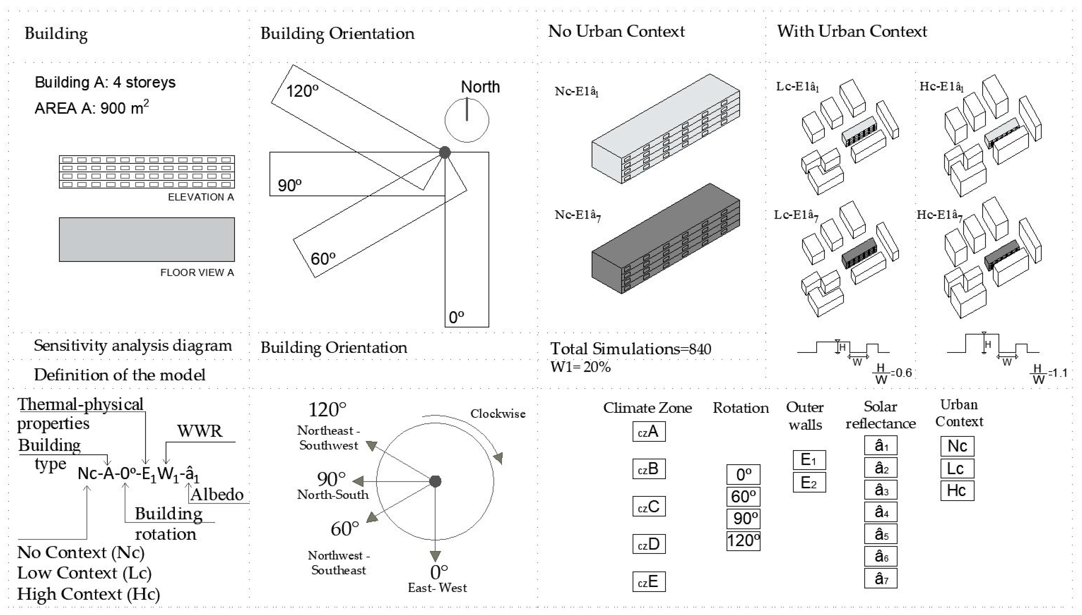
2.1. Building Types, Parameters Used in the Simulations, and Climate Zones
In order to consider the most representative building type within the residential building stock in Spain, the classification resulting from the analyses of statistical data obtained from the Rehenergy project [
69] and from the Spanish National Statistics Institute (INE data base [
70]) was used, with a focus on multi-dwelling units (MDUs). In the research work developed by Fernandez et al. [
68], building A is the optimum one since this building has the lowest heating and cooling demands among the other three configurations proposed. It corresponds to a 60-m long, 15-m wide, and 11.20-m high linear building. It consists of four stories with dwellings, whose usable floor area (UFA) is 80 m
2 and a height equal to 2.8 m. Its volume is 10,080 m
3, with the external surface area of the envelope being 2580 m
2 and its shape factor equal to 0.26.
As mentioned in the introduction, this study was based on dynamic simulations carried out using the Energy Plus software and the Design Builder graphical interface [
71]. In
Figure 1, a first set of simulations accomplished on 840 models considers the parametric variations of climate zones (5), building orientation (4), U-values of the external walls (2), solar reflectance values (7), and different urban contexts (3). With regard to such a group of simulations, the parameter held constant was the window-to-wall ratio (WWR). A constant value of 20% was used for every façade. Users have found the windows to be too small when the WWR is lower than 20% and too large when it is higher than 35% [
72].
Table 1 summarizes all the simulation parameters considered. In the research work carried out by Fernandez et al. [
68], the selection of the following design parameters was justified: Building type, building orientation, U-value, WWR, and climate zone considered. Two new parameters were included and are described in
Section 2.2. They are the solar reflectance and urban context.
Simulations were carried out using the set back and set point temperature schedules presented in
Table 2, i.e., the heating and cooling ideal loads supposed to be in use whenever needed to keep the indoor air temperature within a specific temperature range (17 to 20 °C during the winter and 25 to 27 °C during the summer, respectively).
The first parameter considered was the building orientation. The different building orientations selected for the models were taken from the Spanish Building Technical Code (SBTC). In order to define the type of building orientation of the different models, the 0° value corresponded to an east–west orientation, whereas the 60° value corresponded to a northwest–southeast orientation. In addition, the value equal to 90° corresponded to the north–south orientation and the 120° value related to the northeast–southwest orientation.
The second parameter considered was the thermal transmittance (i.e., U-value, in W m
−2 K
−1), which determines the heat loss through a unit area of different multi-layer envelope elements. In total, 68% of the current building stock in Spain was constructed before 1979 [
73]. Therefore, two different thermal transmittance values were considered for the external walls, while keeping constant the U-values pertaining to the roof and to the windows. The value of 1.58 W m
−2 K
−1 corresponded to those buildings constructed before the above-mentioned regulation came into force, and the value of 0.35 W m
−2 K
−1 corresponded to those built later.
Table 3 describes all the transmittance values of thee walls, roof, and windows in order. Roofs with a slope were not analyzed because their parametric modeling can cause numerical problems during simulations [
74,
75,
76].
The third parameter varied during the simulations was the window-to-wall ratio (WWR). The WWR in the façade is a determining factor in terms of heat gains and losses through glazed surfaces. In order to define this variable, SBTC 2006 was taken as a reference. The selected percentages ranged from 21% to 30% and from 31% to 40%. It was considered that these values cover the usual spectrum of WWR in Spain [
77]. Regarding the WWR, research indicates that when it is less than 20%, it is considered a small value, whereas values higher than 35% are considered too large [
72].
The climate zones established in the Basic Document of Energy Saving pertaining to the Technical Building Code (DB-H) [
78] were identified according to the expected energy demand of buildings and gave rise to a total of 17 zones. Therefore, the selection of zones A4 (very hot climate zones), B4 (hot climate zones), C4 (moderate climate zones), D3 (cold climate zones), and E1 (very cold climate zones) was considered. The representative cities for each zone were Almeria (latitude 36.85, longitude −2.38) within zone A4 and Seville (latitude 37.42, longitude −5.9) within zone B4. Caceres (latitude 39.47, longitude −6.33), Madrid (latitude 40.45, longitude −3.55), and Burgos (latitude 42.35, longitude −3.67) were considered within climate zones C4, D3, and E1 respectively.
2.2. Solar Reflectance and Urban Context
The solar reflectance index (SRI) [
79] is a measure of the constructed surface’s ability to reflect solar energy from its surface back into the atmosphere. The value of the solar reflectance index falls between 0 and 1. A 0-value indicates that the material absorbs all the incident solar energy and it corresponds to a standard black surface (i.e., a non-reflective material capable of emitting the absorbed heat), which results in an increment in temperature of 50 °C under full sun. The 1-value indicates the total reflectance of the constructed surface and it corresponds to a standard white surface (i.e., a completely reflective material, although it is capable of emitting a little stored heat) and therefore resulting in a temperature increment of 8 °C under the same insolation conditions. Due to their ability to reflect solar heat and limit the heating of the building environment, construction products used in coating applications can contribute to reducing the need for air conditioning in hot and sunny climate zones. On the other hand, it also contributes to reducing the effect of an urban heat island (UHI) within the same climate zones.
Table 4 shows the absorptivity values selected for this study [
78]. A low albedo value (â) is 0.04 (i.e., pertaining to dark colors), whereas a high albedo value (â) is 0.8 (i.e., pertaining to light colors). The gray-shaded values are those used in the simulations.
In the Mediterranean climate, the UHI effect is beneficial on the heating demand and the effect of the irradiation obstruction on the cooling demand, with values of the height to the width ratio (H/W) of the building between 0.4 and 1.6 [
80]. Therefore, a dense and compact urban design can help reduce the demand in the Mediterranean climate, demonstrating the validity of the principles of the vernacular architecture and the efficiency of “density” in such a climate context. Due to this occurrence, the authors decided to define the H/W parameter [
81].
The height to width ratio of the urban canyon (H/W) refers to the average height of the urban canyon with respect to the width of the urban canyon).
- -
Low H/W values of the urban canyon (H/W = 14/23 = 0.6).
- -
High H/W values of the urban canyon (H/W = 24.5/23 = 1.1).
2.3. Aerothermal Energy
It is intended that energy from renewable sources in the final gross consumption of energy will be 20% by 2020 according to the European Union regulations [
82]. With regard to this fact, Directive 2009/28/EC [
83] of the European Parliament proposes a procedure by which a heat pump can be considered as energy from renewable sources (please see Equations (1) and (2)):
First, this requires taking into account the efficiency of the energy system, η. Such efficiency can be computed as the ratio of the gross electricity production to the primary energy consumption regarding electricity production. It is calculated as an average in the EU based on Eurostat data and it serves to determine the minimum threshold value of the pump’s seasonal performance factor (SPF) to be considered as renewable (SPF = 1.15 × 1/η). The European Commission sets the η value at 0.455 so the minimum threshold value of the SPF turns out to be 2.5. Second, the estimated amount of useful energy provided by the heat pump (called usable Q) must also be taken into account. It is the estimated total useful heat provided by the pump for domestic hot water (DHW), heating, and cooling production. Finally, the estimated average SPF for electrically driven heat pumps calculated according to the seasonal coefficient of performance in active mode without using a backup electric heater (SCOPnet) must also be considered. With regard to the energy efficiency of a building, the seasonal coefficient of performance (SCOP) is the ratio of the heating equipment’s power output to the electrical power input.
Regarding the calculation carried out, the first step consisted of verifying that the SPF (SCOPnet) of the pump exceeds the minimum value so that it can be considered as renewable (SFP > 2.5 for electrically-driven heat pumps).
In the case that the SCOPnet value is not available [
84], the following Equation (3) can be used:
where FW = weighting factor according to the climate zone considered and FC = correction factor according to the temperature considered.
Once it is confirmed that the heat pump is renewable because the SPF value is greater than 2.5, then it is necessary to justify that the CO
2 emissions (Equation (4)) and the non-renewable primary energy consumption due to the alternative installation (i.e., the aerothermal heat pump) are equal to or lower than those obtained through the solar thermal installation and the auxiliary support system:
The heat pump is considered in several European directives, such as the Energy Efficiency of Buildings. It states that in new buildings, the member states will ensure that, before construction begins, its viability is considered and therefore the technical, environmental, and economic alternative high-efficiency facilities, such as the heat pump, are taken into account.
3. Results
This section presents the results of the 840 simulations accomplished for the different climate zones. In total, 68% of the current building stock in Spain was constructed before 1979 [
73], with transmittance values of U = 1.58 W m
−2 K
−1. Due to this reason, the sample of results corresponds to model A with values of U = 1.58 W m
−2 K
−1. Model A was also simulated using values of U = 0.35 W m
−2 K
−1. It was shown that the results show lower temperature differences and lower demands.
The calculation of the results is presented in three sections. The first section indicates the influence of solar reflectance on the indoor operative temperature (OT). The second analyzes the relationship between the heating demand (Q-heat), cooling demand (Q-cool), and total energy demand (i.e., heating and cooling demands, Q-total). Models without an urban context (Nc), with a low-density urban context (Lc), and a high-density urban context (Hc) are considered. The third one indicates the savings obtained when introducing aerothermal energy.
3.1. Calibration of Models
As a measure of quality control of the simulation outcomes, the results of this research work were preliminarily checked by Fernandez et al. [
68]. The results were corroborated by the Spanish Institute of Energy Diversification and Saving (I) [
85].
3.2. Indoor Operative Temperature Profiles and Evolution
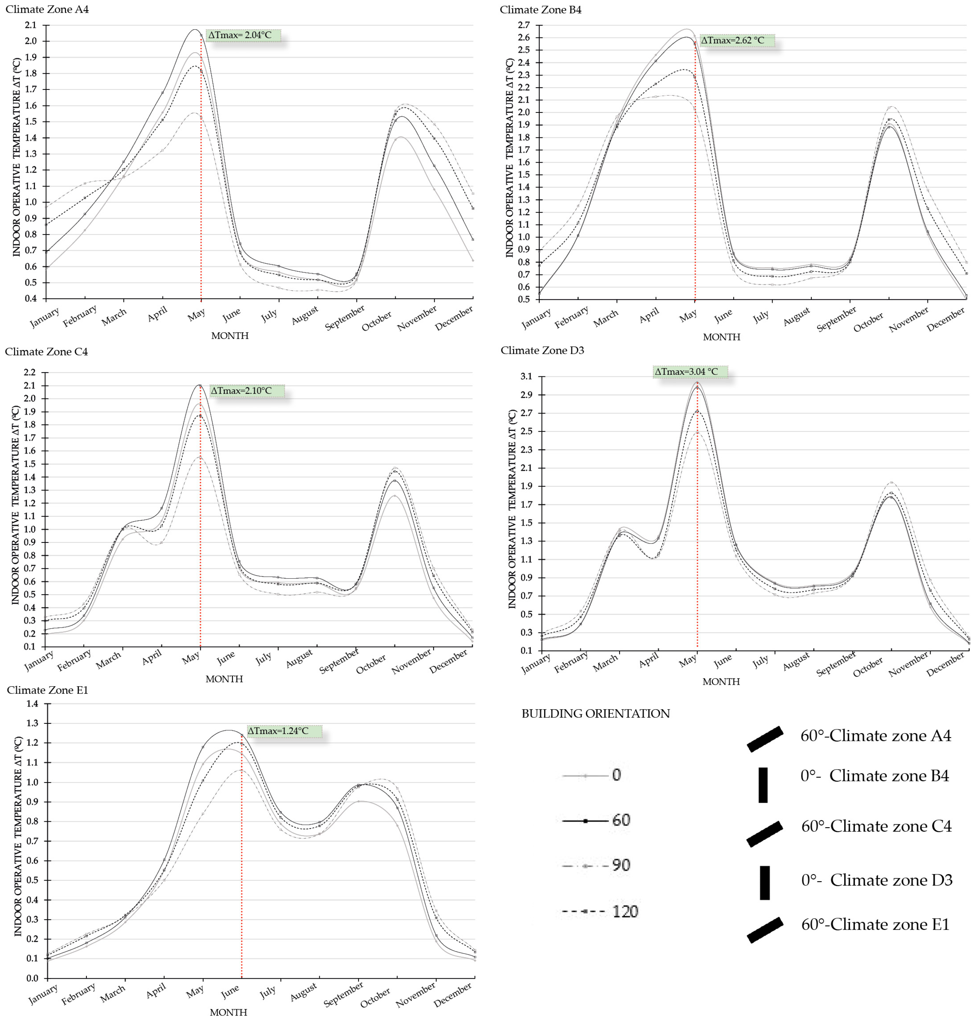
Figure 2 summarizes the monthly average temperature increments (ΔT) in the indoor operative temperature (OT) with respect to the albedo values (â). Dark colors (â7 = 0.04) yield higher temperature values (Tâ7). On the contrary, light colors (â1 = 0.8) imply lower temperature values (Tâ1). Therefore, the following equation was established: ΔT (in °C) = Tâ7 − Tâ1 (+). It can be noted that the increments in temperature are presented with a positive sign (+). The results show the maximum and the minimum increments in temperature found for each climate zone on a monthly basis. Thus, ΔT
max refers to the maximum monthly temperature increment and ΔT
min means the minimum monthly temperature increment.
Regarding very hot climate zones (A4), temperature increments are higher than 2 °C during 11% of the year. Considering the north–south orientation, the highest increment occurs during October, in which the average temperature varies 1.57 °C (i.e., from 27.78 to 26.21 °C). During May, the average temperature varies 1.81 °C when the building orientation is northeast–southwest and it turns out to be 1.90 °C when the orientation is east–west. Furthermore, when the model is oriented northwest–southeast, the maximum average indoor operative temperature variation is 2.04 °C (i.e., from 27.71 to 25.67 °C).
With regard to hot climate zones (B4), the variations of temperature are higher than 2 °C during 22% of the year. During April, the average temperature varies 2.13 °C (i.e., from 24.89 to 22.77 °C) when the building is north–south-oriented. In May, the results show 2.29 °C when the building orientation is northeast–southwest and 2.55 °C when it is northwest–southeast-oriented. Additionally, when the building orientation of the model is east–west, the maximum average indoor operative temperature decreases by 2.62 °C (i.e., from 29.31 to 26.69 °C).
Considering moderate climate zones (C4), during 7% of the year there are increments in temperature that happen to be higher than 2 °C. In May, the average temperature varies 1.55 °C, (from 24.10 to 22.55 °C) when the building orientation is north–south and it varies 1.87 °C when the building orientation is northeast–southwest, whereas it happens to be 1.96 °C when the building orientation is east–west. The maximum average indoor operative temperature varies 2.10 °C (from 25.86 to 23.76 °C) when the building orientation is northwest–southeast.
With regard to cold climate zones (D3), during 13% of the year there are differences in temperature higher than 2 °C. During the month of May, the average temperature varies 2.49 °C (i.e., from 25.9 to 23.41 °C) when the building is north–south-oriented. The increment is 2.72 °C when the building orientation is northeast–southwest and it turns out to be 2.98 °C when the building orientation is northwest–southeast. In addition, the maximum average indoor operative temperature variation is 3.04 °C (from 27.69 to 24.65 °C) when the building orientation is east–west during the month of May. As for very cold climate zones (E1), variations of temperature higher than 2 °C are found only during 0.5% of the year. The maximum temperature differences are found in this case during the month of June. The variation in June is 1.06 °C (from 21.34 to 20.28 °C) when the building is north–south-oriented; it is 1.14 °C when the building orientation is east–west, and it varies 1.20 °C when the building orientation is northeast–southwest. Finally, the maximum increment in June turns out to be 1.24 °C (i.e., from 22.43 to 21.19 °C) when the building orientation is northeast–southwest.
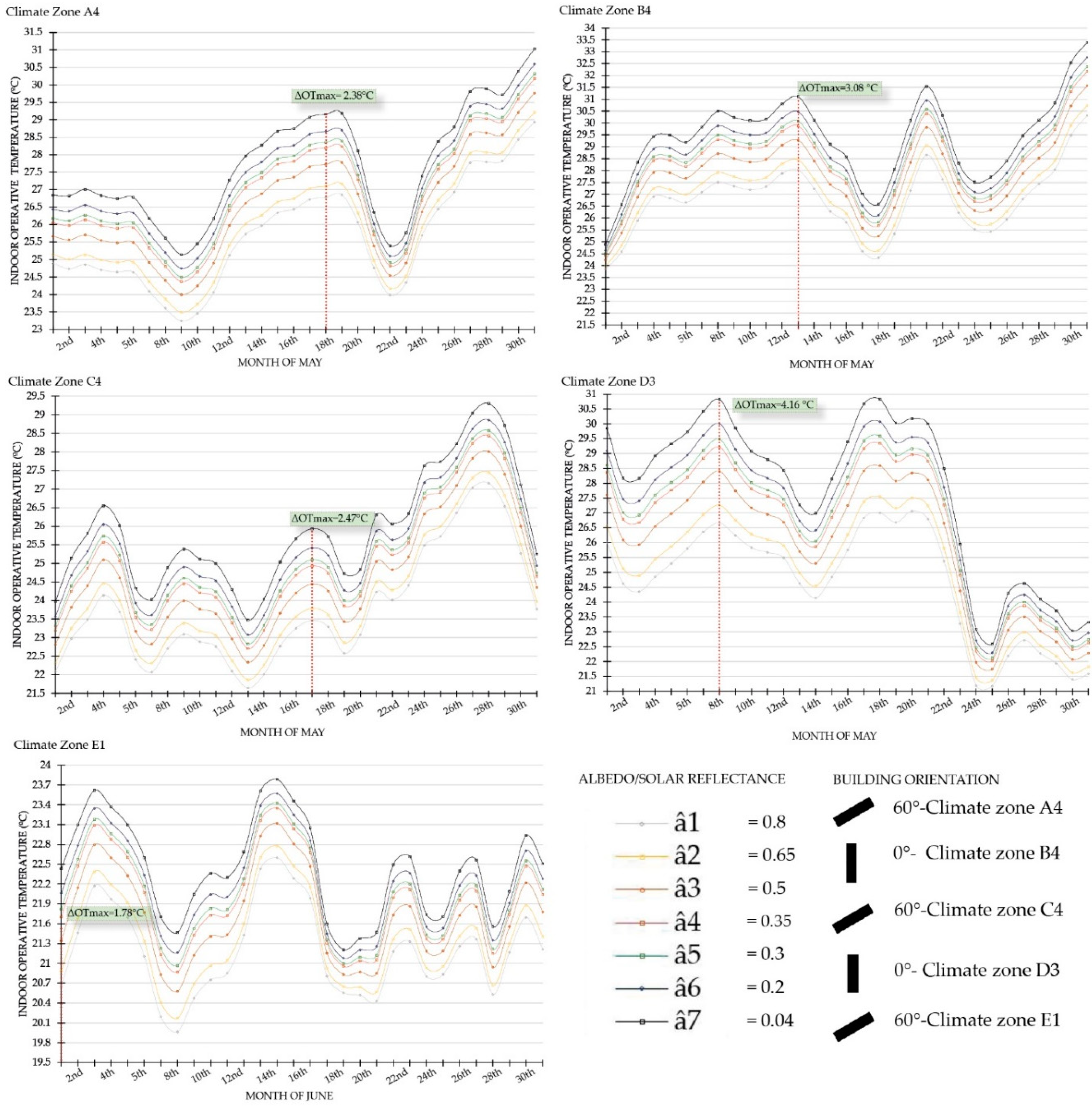
The results of the indoor operative temperature (OT) values on a daily basis are presented in
Figure 3. Therefore, in this particular case, ΔT
max refers to the maximum daily temperature increment and ΔT
min means the minimum daily temperature increment. With regard to the very hot (A4), moderate (C4), and cold (D3) climate zones, the month considered is May. The day in which the maximum temperature increment is spotted coincides with the month in which the maximum temperature increment is found. The highest increment pertaining to very hot climate zones (A4) corresponds to 18 May, in which the increment happens to be 2.38 °C (i.e., 29.16 to 26.78 °C). Considering moderate climate zones (C4), the day spotted is 17 May, in which the temperature increment is 2.47 °C (i.e., 25.24 to 23.77 °C). The highest value of 4.16 °C (from 30.83 to 26.66 °C) is found within cold climate zones (D3) on 8 May.
On the contrary, regarding the hot (B4) and very cold (E1) climate zones, the day in which the maximum temperature difference is found does not belong to the month in which the maximum average temperature increments are found. In the case of hot climate zones (B4), the greatest temperature variation corresponds to 8 April, in which 3.39 °C is observed (from 29.74 to 26.35 °C). During the month of April, the average temperature variations are 2.13 °C when the building orientation is north–south. As mentioned above, the maximum average temperature increments are found within the month of May. Therefore, on 13 May, there are temperature increments of 3.08 °C (from 31.10 to 28.02 °C). Finally, with regard to very cold climate zones (E1), the highest average temperature variation corresponds to 1 June. In this particular case, the value is 1.78 °C (from 22.43 to 20.66 °C) although the day with the highest temperature difference is 31 May, whose value is 2.21 °C (from 24.15 to 21.94 °C).
After analyzing the previous results of Spain’s climate zones, it is noted that when the albedo levels of the façade are increased from dark-colored values (â7 = 0.04) to light-colored values (â1 = 0.8), the indoor operative temperature values are reduced during the summer months. On the contrary, during the winter months, it is noted that the albedo levels of the façade must be reduced in order to increase the indoor operative temperatures.
3.3. Climate Cross-Comparison
As mentioned above, the increment in the albedo levels from dark-colored values (â7 = 0.04) to light-colored values (â1 = 0.8) decreases the indoor operative temperatures.
Table 5 shows the comparison between models with lower reductions of indoor operative temperatures and those with the greatest reductions in the OT values. It is observed that the orientations of the buildings considered vary depending on the climate zone considered. In the case of very hot climate zones (A4), the smallest reduction in the OT values corresponds to the optimal building orientation in Spain according to Fernandez et al. [
68] which is north–south, and it turns out to be ΔT
min = 0.45 (from 26.9 to 26.5 °C).
On the contrary, considering the remaining climate zones, the models with lower differences in indoor operative temperatures according to the albedo levels of the façade correspond to the model whose building orientation is east–west. Thus, the values are ΔTmin = 0.5 relating to hot climate zones (B4) from 19.6 to 19.1 °C, ΔTmin = 0.14 relating to moderate climate zones (C4) from 18.7 to 18.5 °C, ΔTmin = 0.18 relevant to cold climate zones (D3) from 18.5 to 18.3 °C, and ΔTmin = 0.1 pertaining to very cold climate zones (E1) from 18.3 to 18.2 °C. Regarding the models in which there are higher temperature differences according to the albedo levels of the façade, the following results are obtained. As for cold climate zones (D3), the monthly average temperature is 3.04 °C when the building orientation is east–west. The opposite values are found when considering very cold climate zones (E1), in which the monthly average temperature is 1.24 °C when the building orientation is northwest–southeast. These results show the different behaviors of the albedo levels within the climate zones considered in Spain.
3.4. Analysis of the Energy Demand According to the Different Climate Zones
The results refer to both the heating and cooling demand, as well as the total energy demand. The heating and cooling losses were not taken into account. This selection is related to the construction of zero energy buildings within the European Union and focuses on the use of technologies relating to energy efficiency systems.
Figure 4,
Figure 5,
Figure 6,
Figure 7 and
Figure 8 show the heating and cooling energy demands in the different climate zones considered within this research work. The following parameters remain constant: The type of building (A), shape factor (0.26), WWR equal to W1 (20%), and U-value (1.58 W m
−2 K
−1). The saving and penalties observed are detailed in
Figure 9. The criterion selected for defining the best design solution was that of the lowest values of energy demand pertaining to cooling (Q–cool), heating (Q–heat), and the total energy demand (both heating and cooling, Q-total). The opposite applies for identifying the worst design solutions.
Figure 4,
Figure 5,
Figure 6,
Figure 7,
Figure 8 and
Figure 9 indicate the best and worst option respectively in terms of Q-total with and without consideration of the urban context.
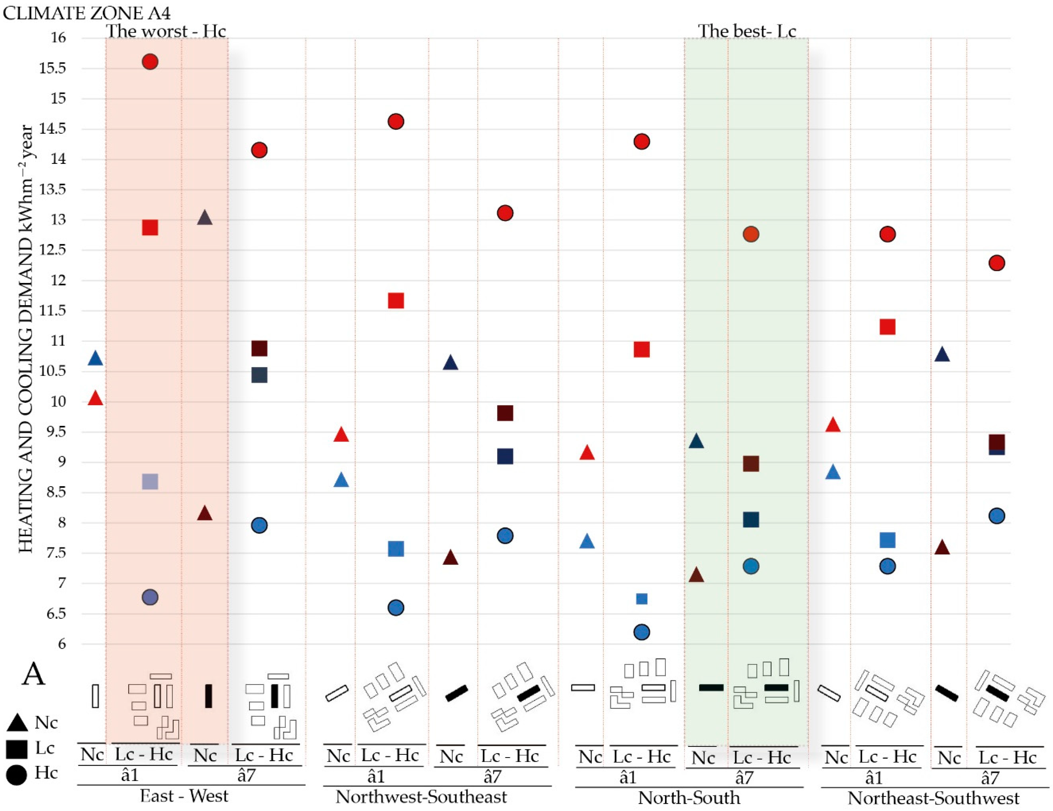
3.4.1. Very Hot Climate Zones (A4)
Figure 4 shows the analysis of the results pertaining to very hot climate zones (A4). It can be noted that the lowest heating energy demand (Q-heat = 7.16 kWh m
–2) is found when using dark colors (â
7 = 0.04), when the building orientation is north–south, and when the urban context is not considered. On the other hand, the lowest cooling demand (Q-cool = 6.20 kWh m
−2) is found in the model with a high urban canyon (1.1), light colors (â
1 = 0.8), and when the orientation considered is north–south. Therefore, the most common parameter in both cases is the building orientation, which is north–south. The lowest heating demand is found when the urban context is not considered whereas that of the cooling demand is found when the urban context is taken into account.
The worst model considering the highest heating demand (Q-heat = 15.61 kWh m–2) corresponds to the model with a high urban canyon (1.1), light colors (â1 = 0.8), and when the building orientation is east–west. As for the cooling demand (Q-cool = 13.05 kWh m−2), the value corresponds to the model without an urban context when the building is east–west-oriented and dark colors are used (â7 = 0.04). On the contrary, in this particular case, the lowest heating demand is found when the urban context is considered whereas that of the cooling demand is found when the urban context is not taken into account. East–west orientation is the common parameter in terms of obtaining the more unfavorable results.
On the other hand, regarding the total energy demand, the difference in the values obtained without an urban context and with a low urban canyon range from 0.51 to 1.2 kWh m−2 per year.
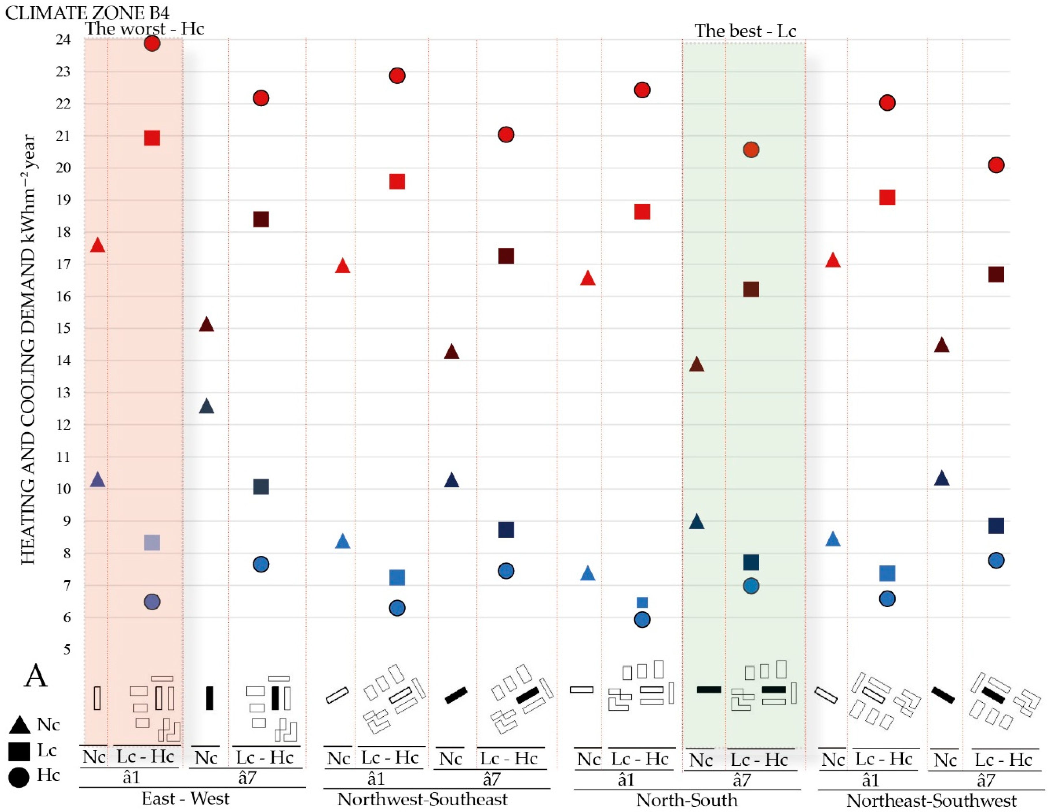
3.4.2. Hot Climate Zones (B4)
Figure 5 shows the analysis of the results pertaining to hot climate zones (B4). The best model regarding the lowest heating demand (Q-heat = 13.90 kWh m
−2) corresponds to a model without consideration of an urban context when the building orientation is north–south and dark colors are used (â7 = 0.04). It corresponds to the same characteristics relevant to those of very hot climate zones (A4). The best model pertaining to the lowest cooling demand (Q-cool = 5.94 kWh m
−2) corresponds to the model with a high urban canyon (1.1) when it is north–south-oriented and light colors are used (â1 = 0.8).
The worst model considering the highest heating demand (Q-heat = 23.88 kWh m−2) corresponds to the model with a high urban canyon (1.1) when the building orientation is east–west and light colors are used (â1 = 0.8). As for the cooling demand (Q-cool = 12.60 kWh m−2), it corresponds to a model without an urban context when the building orientation is east–west and dark colors are used (â7 = 0.04). All the remaining parameters are equal to those pertaining to very hot climate zones (A4).
As for the total energy demand, the differences obtained with and without consideration of the urban contexts range from 1.03 to 2.45 kW h−2 per year in hot climate zones (B4). A discrepancy is found when dealing with very hot climate zones (A4), since although the most unfavorable isolated model corresponds to the same orientation as that of very hot climate zones (A4), in this particular case, the solar reflectance corresponds to light colors (â1 = 0.8). Therefore, this variation in the solar reflectance values occurs when varying from the very hot (A4) to the hot (B4) climate zones.
3.4.3. Moderate Climate Zones (C4)
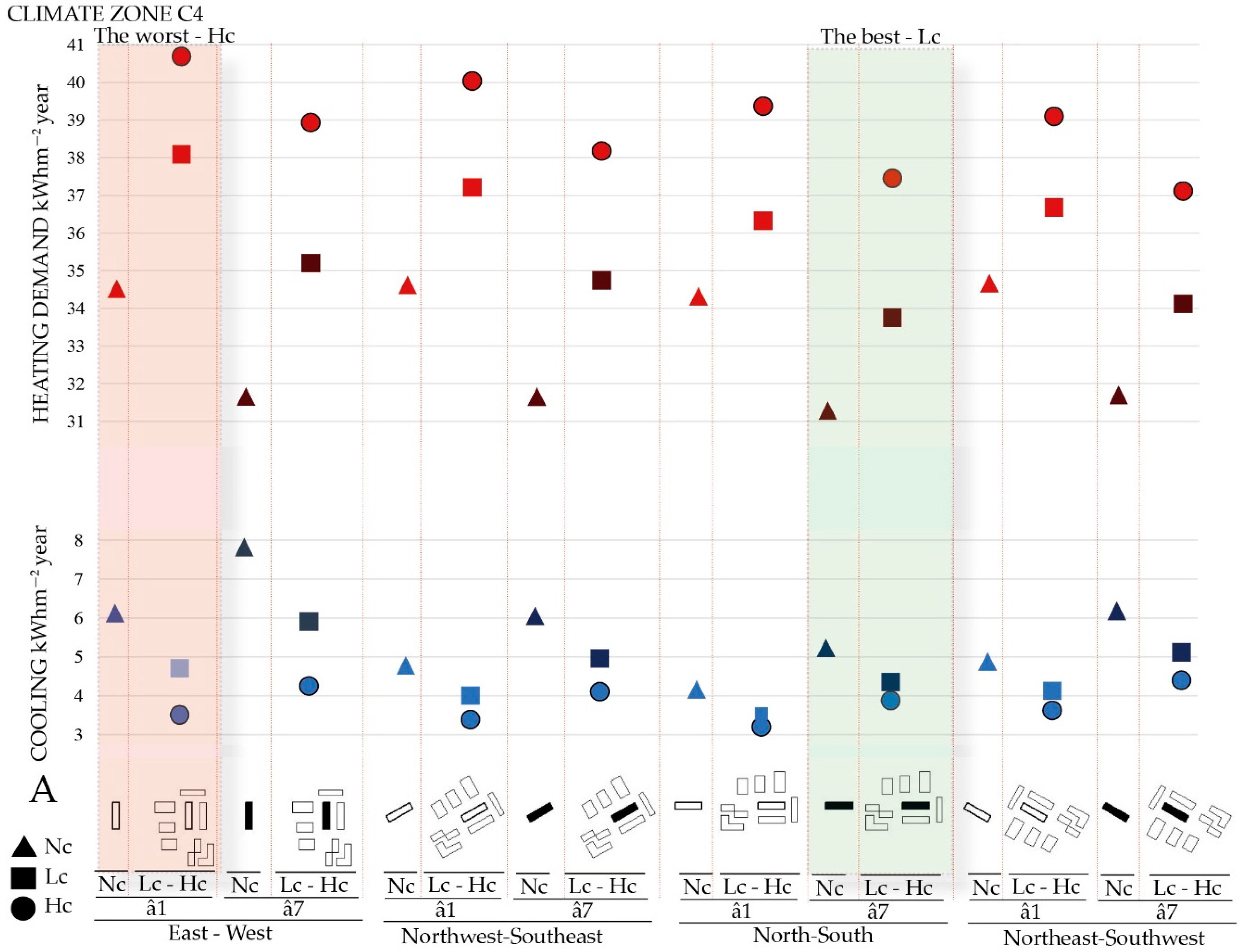
Figure 6 shows the analysis of the results pertaining to moderate climate zones (C4). The best model within moderate climate zones (C4) is the same as that obtained within the very hot (A4) and hot (B4) climate zones. The lowest heating demand (Q-heat = 31.28 kWh m
−2) corresponds to the model without urban context when it is north–south-oriented and light colors are used (â1 = 0.8). On the other hand, the lowest cooling demand (Q-cool = 3.20 kWh m
−2) is associated to the model with a high urban canyon (1.1) when it is north–south-oriented and light colors are used (â1 = 0.8).
Considering the heating demand, the worst model coincides with that of the very hot (A4) and hot (B4) climate zones (Q-heat = 40.69 kWh m−2). It corresponds to the highest heating demand associated to the model with a high urban canyon (1.1) when the building orientation is east–west and light colors are used (â1 = 0.8). As for the cooling demand, it coincides with the worst model pertaining to the very hot (A4) and hot (B4) climate zones. The highest cooling demand (Q-cool = 7.82 kWh m−2) is associated with the model without consideration of the urban context when the building orientation is east–west and dark colors are used (â7 = 0.04).
As for the total energy demand (Q-total), the differences obtained with and without consideration of the urban contexts range from 1.6 to 3.6 kW h−2 per year. It can be noted that the colder the climate zones considered, the greater such differences are.
3.4.4. Cold Climate Zones (D3)
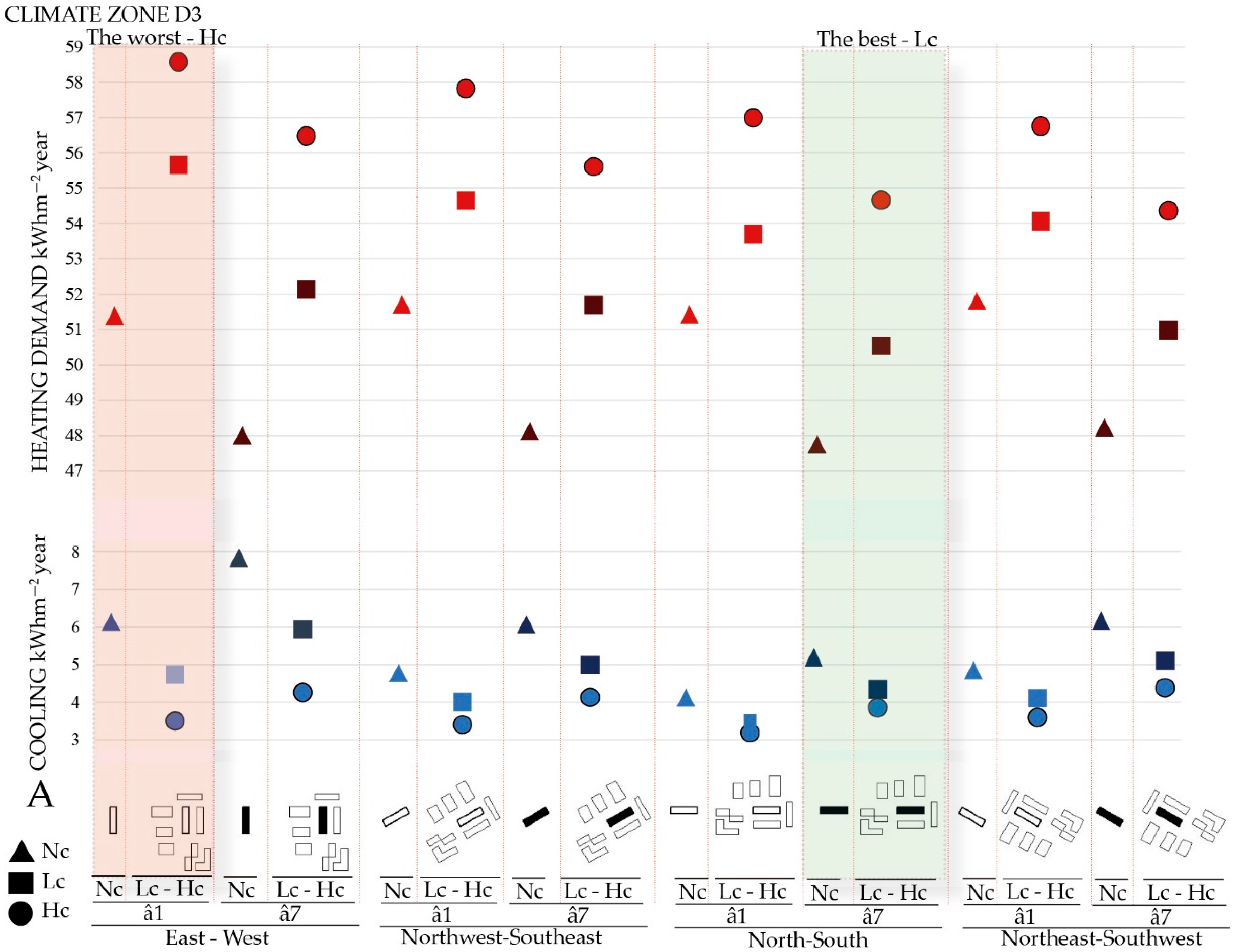
Figure 7 shows the analysis of the results pertaining to cold climate zones (D3). The lowest heating demand within cold climate zones is the same one as those obtained within very hot (A4), hot (B4), and moderate (C4) climate zones. It corresponds to the model without an urban context when the building orientation is north–south and dark colors are used (â
7 = 0.04). This corresponds to model N
C-90°–E1â
7 with a value of the heating demand equal to 47.75 kWh m
−2. However, the lowest cooling demand (Q-cool = 3.19 kWh m
−2) within cold climate zones (D3) corresponds to the model with a high urban canyon (1.1) when using light colors (â
1 = 0.8) and a north–south orientation.
The highest heating demand within cold climate zones (D3) is the same as those of very hot (A4), hot (B4), and moderate (C4) climate zones. This model corresponds to a greater value of the heating demand (Q-heat = 58.58 kWh m−2) associated to the model with a high urban canyon (1.1) when the building orientation is east–west and light colors are used (â1 = 0.8). The highest cooling demand coincides with those of very hot (A4), hot (B4), and moderate (C4) climate zones. In this case, a greater value of the cooling demand is associated to the model without an urban context when the building orientation is east–west and the use of dark colors (â7 = 0.04). This corresponds to model NC -0°-E1â7 with a value equal to 7.83 kWh m−2 and it is associated with the model without an urban context when the building orientation is east–west and dark colors are used (â7 = 0.04).
With regard to the total energy demand (Q-total), it happens to be the same as those of hot (B4) and moderate (C4) climate zones. In this particular case, the differences range from 1.93 to 4.57 kWh m−2 per year. The results found in hot (B4), moderate (C4), and cold (D3) climate zones show similar behaviors in terms of the minimum and maximum values of the total energy demand.
3.4.5. Very Cold Climate Zones (E1).
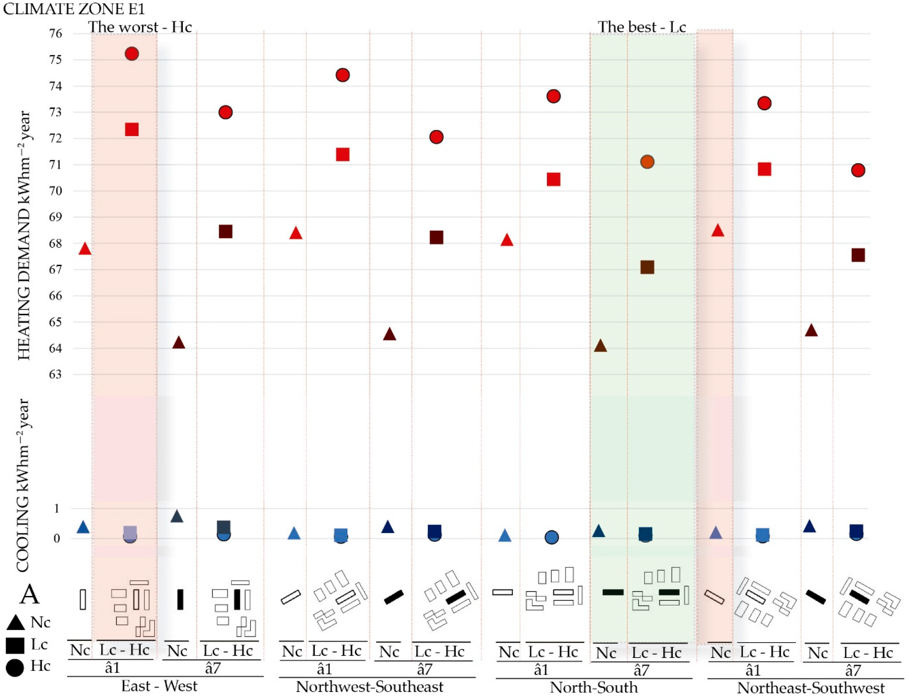
Figure 8 shows the analysis of the results pertaining to very cold climate zones (E1). With regard to the lowest heating demand (Q-heat), the best model corresponds to the model without an urban context when the building orientation is north–south and dark colors are used (â7 = 0.04). In this case, the value of the heating demand equals 64.12 kWh m
−2. A slight variation is found when the building orientation considered is east–west (64.24 kWh m
−2). However, the lowest cooling demand within very cold climate zones (Q-cool = 0.04 kWh m
−2) corresponds to the model with a high urban canyon (1.1) when it is north–south-oriented and light colors are used (â1 = 0.8).
The highest heating demand within very cold climate zones (E1) is the same as those of the above-mentioned climate zones. It corresponds to the highest heating demand (Q-heat = 75.29 kWh m−2), which is associated with the model with a high urban canyon (1.1) when the building orientation is east–west and light colors are used (â1 = 0.8). It coincides with the worst model pertaining to very hot (A4), hot (B4), moderate (C4), and cold (D3) climate zones. The highest cooling demand (Q-cool = 0.75 kWh m−2) is associated with the model without an urban context when the building orientation is east–west and using dark colors (â7 = 0.04).
With regard to the total energy demand (Q-total), the best model is the same as those of hot (B4), moderate (C4), and cold (D3) climate zones. On the contrary, the most unfavorable models are found when the urban context is not considered, and the orientation is northwest–southeast. Finally, in very cold climate zones (E1), the maximum differences are obtained. Such values range from 2.74 to 6.58 kWh m−2 per year.
3.5. Climate Cross-Comparison
Table 6 shows the comparison between the optimal models and the worst ones with respect to the different climate zones. Regarding the optimal models, the following results are shown. Fernandez et al. [
68] defined the optimal Q-heat model, which is Nc-A-90°-E2w1â2 without an urban context, when the building orientation is north–south and envelope E2 (U = 0.35 W m
−2 K
−1) is used, as well as an WWR equal to W1 (20%), dark colors (0.2), and a lower shape factor (0.26). This research work showed that this tendency is similar in all climate zones within Spain. As for the Q-cool, it is demonstrated that high urban canyons provide lower values of energy demand. Regarding the total demand (Q-total), the optimal model is Nc-90°-E1â7 without an urban context, when the building orientation is north–south and envelope E1 (U = 1.58 W m
−2 K
−1) is used, dark colors (0.04), and a lower shape factor (0.26). Fernandez et al. [
68] defined that light colors are beneficial for very hot (A4), hot (B4), and moderate (C4) climate zones, whereas dark colors are beneficial for cold (D3) and very cold (E1) climate zones.
With respect to the most unfavorable models, the following results are shown. As for Q-heat, the light colors and shady spots projected by the neighboring buildings imply that higher heating demands are required. As for Q-cool, the worst configuration corresponds to lower albedo levels (0.04), which is associated with light colors. According to Fernandez et al. [
68], the most unfavorable option corresponds to higher shape factor values and the use of light colors. If the shape factor is reduced, then dark colors are the most unfavorable option. Because of this occurrence, the shape factor of a building is more influential than the solar reflectance in architectural design. Regarding the total demand (Q-total) and using the same shape factor, the most unfavorable model corresponds to the east–west orientation and light colors in all the climate zones. Thus, the lowest demands pertaining to Q-heat and Q-total are obtained when simulating without consideration of urban contexts. On the contrary, in order to achieve lower values of Q-cool, high urban contexts (Hc = 1.1) must be considered.
3.6. Heating and Cooling Demands with Their Related Savings and Penalties
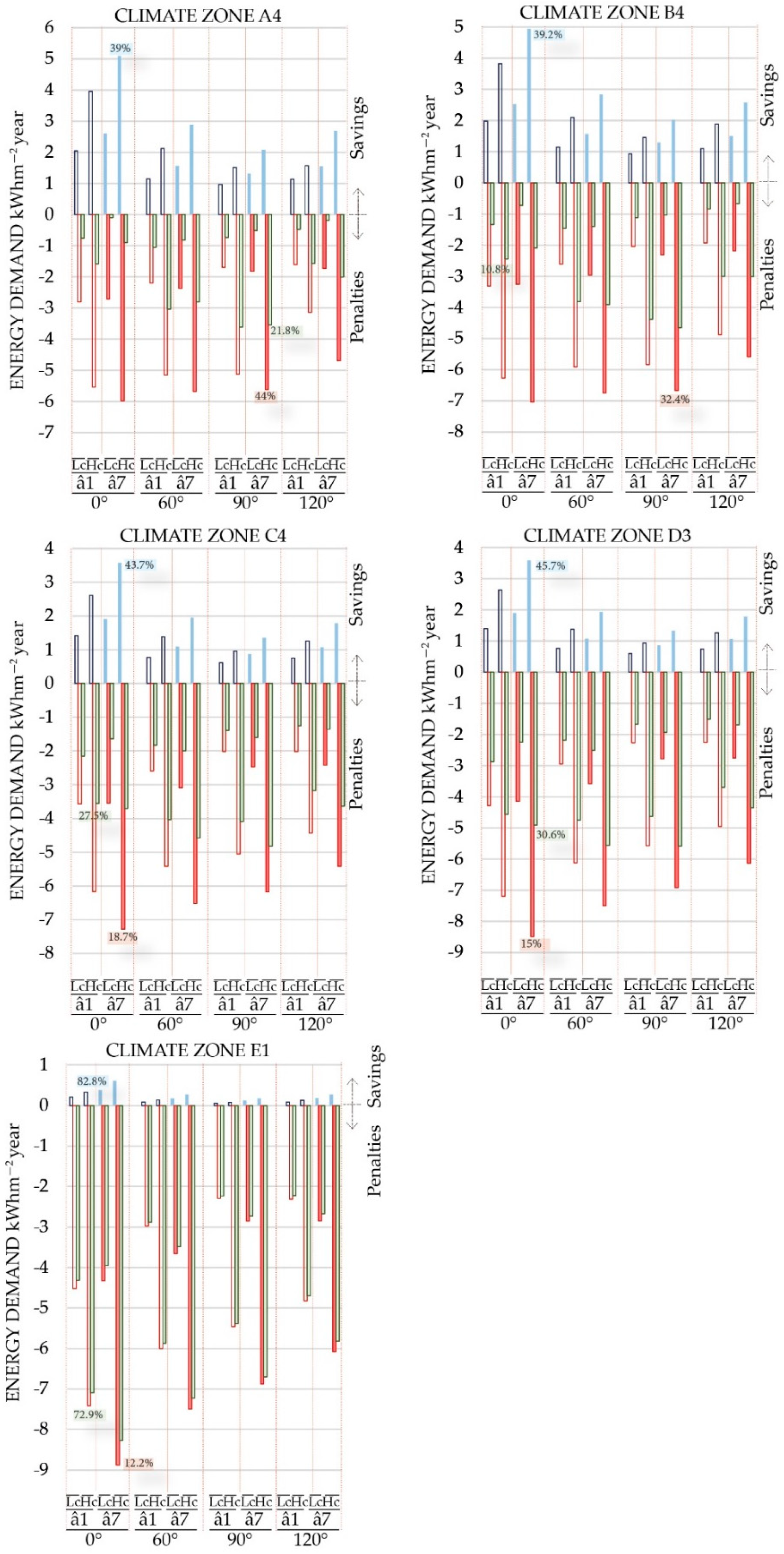
Figure 9 summarizes the differences in the energy demand expressed in kWh m
−2. Results with and without consideration of the urban context are compared, as well as the use of a high and a low urban canyon. The increase in the energy demand is represented by a negative sign (−), since it is considered a penalty, and the decrease in the energy demand is represented by a positive sign (+), since it is considered a saving. In order to show the results, the authors classified the architectural design parameters through a sensitivity analysis. The sensitivity index for each parameter was calculated by using the following expressions:
Q-heat sensitivity index without an urban context—with an urban context (in kWh m−2) means Q-heat X-best—Q-heat X-worst (penalties and negative values).
Q-cool sensitivity index without an urban context—with an urban context (in kWh m−2) means Q-cool X-worst—Q-cool X-best (savings and positive values).
In order to find the sensitivity index considering an urban context, the best Q-heat or Q-cool must be subtracted from the worst Q-heat or Q-cool and divided by the worst Q-heat or Q-cool expressed as a percentage.
X-best refers to the lowest demand values for all design combinations, including the best performing value of both low and high urban contexts.
X-worst refers to the highest demand values for all design combinations, including the worst performing value of both low and high urban contexts.
The simulation with an urban context has a negative impact on the heating demand (increase in kWh m−2). On the contrary, the simulation with an urban context has a positive impact on the cooling demand (reduction in kWh m−2). Finally, with respect to the total demand, there is always a negative impact (increase in kWh m−2).
Table 7 shows the different sensitivity indexes (in kWh m
−2). The gray-shaded values in
Table 7 correspond to the maximum differences, whereas the underlined values shown in the same table correspond to the minimum ones.
The maximum differences found regarding Q-cool and Q-heat coincide in all climate zones. They correspond to model Hc-0°-E1â7 when using a high urban canyon (1.1), dark colors (â7 = 0.04) and east–west orientation. Regarding the total demand in very hot climate zones (A4), the values correspond to model Hc-90°-E1â1 when using a high urban canyon (1.1), light colors (â1 = 0.8), and north–south orientation. In the hot (B4), moderate (C4), and cold (D3) climate zones, it is noted that the values correspond to model Hc-90°-E1â7 when using a high urban canyon (1.1), dark colors (â7 = 0.04), and north–south orientation. Finally, with regard to very cold climate zones (E1), the values correspond to model Hc-0°-E1â7 when using a high urban canyon (1.1), dark colors (â7 = 0.04), and east–west orientation.
Some of the most significant results are shown below. Regarding very hot climate zones (A4), such a model presents heating penalties equal to 5.61 kWh m−2 (44%) and cooling savings equal to 5.09 kWh m−2 (39%) when using a high urban canyon (1.1), dark colors (â7 = 0.04), and east–west orientation. Regarding the total energy demand, the penalties equal 3.54 kWh m−2 (21.8%) when using a high urban canyon (1.1), light colors (â1 = 0.8), and north–south orientation.
With regard to very cold climate zones (E1), heating penalties equal 8.88 kWh m−2 (12.2%) when using a high urban canyon (1.1), dark colors (â7 = 0.04), and east–west orientation. As for moderate climate zones (C4), cooling savings equal 3.57 kWh m−2 (45.7%) and as for cold climate zones (D3) heating penalties turn out to be 8.48 kWh m−2 (15%).
However, penalties relating to the total energy demand vary according to the climate zone considered. Taking into account hot climate zones (B4), penalties equal 4.65 kWh m−2 (10%) when using a high urban canyon (1.1), dark colors (â7 = 0.04), and north–south orientation. Similarly, regarding moderate climate zones (C4), penalties equal to 3.56 kW h−2 (27.5%) are found. With respect to cold climate zones (D3), the penalized values happen to be 5.58 kW h−2 (13%). Finally, considering very cold climate zones (E1), penalties equal to 7.09 kWh m−2 (72.9%) correspond to the use of a high urban canyon (1.1), dark colors (â7 = 0.04), and east–west orientation.
The minimum differences found regarding Q-cool correspond to model Lc-90°-E1â1 when using a low urban canyon (0.6), light colors (â1 = 0.8), and a north–south orientation. However, the minimum differences found regarding Q-heat correspond to very hot (A4), hot (B4), moderate (C4), and cold (D3) climate zones when using model Lc-120°-E1â1 and considering a low urban canyon (0.6), light colors (â1 = 0.8), and northeast–southwest orientation. On the contrary, in the case of very cold climate zones (E1), the minimum differences found regarding Q-heat occur when the building orientation is north–south. Regarding the total energy demand, significant differences are shown depending on the different climate zones. In very hot climate zones (A4), it corresponds to model Lc-0°-E1â7 when taking into account a low urban canyon (0.6), dark colors (â7 = 0.04), and east–west orientation. In hot climate zones (B4), it corresponds to model Lc-120°-E1â7 when using a low urban canyon (0.6), dark colors (â7 = 0.04), and a northeast–southwest orientation. As for the remaining climate zones, the minimum differences are found with model Lc-120°-E1â1 when a low urban canyon (0.6), light colors (â1 = 0.8), and a northeast–southwest orientation are considered.
3.7. Renewable Energies—Aerothermal Energy
Energy savings and penalties were calculated for systems run by electricity, gas, and for an aerothermal system. With regard to the energy efficiency of the building as mentioned above, the seasonal coefficient of performance (SCOP) is the ratio of the heating equipment’s power output to the electrical power input. The seasonal energy efficiency ratio (SEER) is the ratio of the air conditioner’s power output to the electrical power input. The variation of the annual energy demand for the air conditioning and heating systems expressed in kWhm
−2 in Spain is shown below. The cost (€m
−2) refers to a U-value equal to 1.58 W m
−2 K
−1 and an increment in the albedo values from â1 = 0.8 to â7 = 0.04. The gray-shaded values in
Table 8 correspond to the maximum differences, whereas the underlined values shown in the same table correspond to the minimum ones.
Table 8a shows the SCOP and SEER values equal to 1 pertaining to systems run by electricity.
Table 8b shows the SCOP and SEER values equal to 0.7 of systems run by gas.
Table 8c shows values SCOP equal to 3.8 and SEER equal to 4.3 (aerothermal system).
Comparing the tables, the results obtained show that when the simulation considers urban contexts, there are economic savings in the cooling demand by using the following expression: (energy saving in cooling demand × energy cost)/SEER. On the contrary, it produces economic penalties on the heating demand, which are equal to the following expression: (energy penalties in heating demand × energy cost)/SCOP. Regarding the total demand, the results show that penalties will always be obtained.
Regarding the price of electric energy used for the estimates, the price considered was 0.2 €/kWh based on data obtained from the Ministry of Industry and Commerce, 2010 and intended for dwellings with a power consumption lower than 10 kW as per the Spanish regulations. The estimated price of gas is 0.047 €/kWh (European Union, 2010). The price was calculated as an average cost per kWh obtained from the user’s electricity invoice including all taxes (VAT and electricity tax) and including free-market users, who generally pay a higher tariff.
Table 8a shows the maximum savings in the cooling demand pertaining to systems run by electricity. They correspond to model Hc-0°-E1â7 when using a high urban canyon (1.1), dark colors (â7 = 0.04), and the building orientation is east–west. In this particular case, a cost of 1.02 €/m
2a is found in very hot climate zones (A4). However, considering very cold climate zones (E1), the same model presents higher penalties, i.e., 1.78 €/m
2a pertaining to the heating demand and 1.65 €/m
2 relevant to the total demand.
Table 8b shows the maximum savings in the cooling demand relevant to systems run by gas. They correspond to model Hc-0°-E1â7 when using a high urban canyon (1.1), dark colors (â7 = 0.04), and the building orientation is east–west. In this case, a cost of 0.34 €/m
2a is found in very hot climate zones (A4). However, considering very cold climate zones (E1), the same model presents higher penalties, i.e., 0.6 €/m
2a relating to the heating demand and 0.56 €/m
2a in the total demand. Finally,
Table 8c shows the maximum savings in the cooling demand values pertaining to the use of a renewable energy, such as an aerothermal system. It is observed that the maximum savings in the cooling demand correspond to model Hc-0°-E1â7 when using a high urban canyon (1.1), dark colors (â7 = 0.04), and the building orientation is east–west. In this particular case, a cost of 0.24 €/m
2a is found in very hot climate zones (A4). However, considering very cold climate zones (E1), the same model presents higher penalties, i.e., 0.47 €/m
2a pertaining to the heating demand and € 0.44/m
2a relevant to the total demand.
4. Conclusions
The present research work focused on the impact of technology when considering the urban context of a building. This is relevant for the balance of urban albedo levels and indoor thermal comfort. In most studies, simulations were performed without consideration of urban contexts and therefore the effects of solar reflectance and shady spots were not taken into account.
The results obtained through the parametric simulations help understand what the objectives relating to energy efficiency in a project must be. Simulation helps building designers identify the most influential design parameters to be considered. It also allows them to identify the value ranges of the design parameters included in their projects.
One of the limitations of this research work is that it was simulation-based only. However, one of the objectives of this research work was the quantification of the differences in the results according to the variability of parameters. Therefore, as per our viewpoint, this method can be considered adequate although it was simulation-based only.
The increment in the albedo levels (i.e., solar reflectance) of a façade during the winter periods produces minimum differences in the indoor operative temperatures. On the contrary, increasing the albedo levels during the summer period produces maximum temperature differences. Values ranging from 1.24 to 3.04 °C were found depending on the climate zone considered. Therefore, during the winter, a reduction of the albedo values increases the indoor operative temperatures, whereas during the summer, an increment of the albedo values decreases the indoor operative temperatures.
The building orientation influences the maximum temperature differences according to the solar reflectance levels. In the case of very hot (A4), moderate (C4), and very cold (E1) climate zones, the maximum differences were found when the model was northwest–southeast-oriented. On the other hand, in the case of hot (B4) and cold (D3) climate zones, this was found when the model was east–west-oriented. Regarding the minimum temperature differences, the best building orientation was north–south when considering very hot climate zones (A4), whereas in the remaining climate zones the best building orientation was east–west.
Simulation of an urban building in an isolated context (i.e., without its urban context) showed higher cooling than those actually demanded by the building in all climate zones. This is due to the fact that the isolated building receives all possible solar irradiation, since no neighboring building is projecting shady spots on it. Therefore, its cooling demand will be higher and therefore the cooling system might be oversized as the simulated solar irradiation does not reach the real building due to the presence of neighboring buildings.
On the other hand, simulating simulation of an isolated building also showed lower heating demand values than the supply in all climate zones. This is due to the fact that the isolated building receives all the possible solar irradiation, since no neighboring building is projecting shady spots on it. Therefore, its heating demand will be lower and therefore the heating system might be undersized as the simulated solar irradiation does not reach the real building due to the presence of neighboring buildings.
The cooling demand when considering a high urban canyon (1.1) is always lower than when considering a low urban canyon (0.6). The heating demand with a low urban canyon (0.6) is always lower than that of a high urban canyon (1.1). In order to minimize the Q-heat values, it is recommended that dark colors are used. On the contrary, to minimize the Q-cool, light colors must be used. As for the total demand (Q), the lowest values are associated with the use of dark colors. This is due to the fact that the highest demand in a climate, such as Spain, corresponds to the winter months. Thus, the use of light colors is more beneficial for very hot (A4) and hot (B4) climate zones (A4), since higher cooling demand values were found. As for the moderate (C4) and cold (D3) climate zones, similar values of the cooling demand were obtained. In cold (D3) and very cold (E1) climate zones, the use of dark colors is recommended since the heating demand is much higher. However, moderate climate zones (C4) are the most controversial zones at the time of decision making. The differences obtained between simulations with or without consideration of the urban context are more remarkable in the case of the coldest climate zones.
As for the Q-cool, it is noted that a high urban canyon helps reduce the cooling demand. Dark colors favor lower heating demands and total demands whereas light colors favor lower cooling demands.
With respect to the most unfavorable models, the following results are shown. As for Q-heat, light colors and shady spots projected by the neighboring buildings imply that higher heating demands are required. As for Q-cool, the worst configuration corresponds to lower albedo levels (dark colors). The shape factor of a building is more influential than the albedo levels in all climate zones. If building designers want to obtain lower Q-heat and Q-total demands, it is recommended that the building is simulated without an urban context. On the contrary, if designers want to obtain lower Q-cool demands, then a simulation including a high urban context (Hc = 1.1) is recommended.
The simulation with an urban context has a negative impact on the heating demand (i.e., an increment in kWh m−2). On the contrary, simulation with an urban context has a positive impact on the cooling demand (i.e., a reduction of kWh m−2). Finally, with respect to the total demand, simulation with an urban context has a negative impact since higher values of the demand were obtained in all cases (i.e., an increment in kWh m−2). This research work showed the significant importance of urban contexts on the energy demands. Therefore, neighboring buildings play a crucial role and can be considered an important impact variable to be taken into account. Thus, urban contexts substantially affect the Q-cool, showing an increase in the values obtained for all climate zones. On the contrary, in terms of Q-heat and Q-total, the values obtained when considering the urban context were lower than those obtained when simulating the isolated building.
The highest differences between simulating with or without an urban context are described below. The model that considers a high urban canyon when the building orientation is east–west and dark colors are used resulted in an increment in the cooling demand (39% in very hot climate zones) and the heating demand (12% in very cold climate zones).
As for the total demand, it depends on the climate zone considered. In very hot climate zones (A4), the highest difference corresponds to the north–south orientation when using light colors (21.8%), whereas in the remaining zones when using dark colors, the values are 10.8% (hot), 27.5% (moderate), and 30.6% (cold), respectively. As for very cold climate zones (E1), the difference is 72.9% when the building orientation is east–west and dark colors are used.
The smallest differences between simulating with or without an urban context are described below. The model that considers a low urban canyon when the building orientation is north–south and using light colors results in an increment in the cooling demand (i.e., 12.5% in very hot climate zones). A northeast–southwest orientation when using light colors in very cold climate zones results in a lower heating demand (3.3.%).
Similarly, as for the total demand, it depends on the climate zone considered. In very hot climate zones (A4), it corresponds to the east–west orientation and use of dark colors (4.9%). In hot climate zones (B4), it corresponds to the northeast–southwest orientation (1.5%). In the remaining zones, the following results were obtained: 10% (moderate), 11.2% (cold), and 39.6% (very cold) when the building orientation is northeast–outhwest and dark colors are used.
The variation of the solar reflectance values, the building orientation, and the thermal transmittance of the walls results in an energy efficient model in order to optimize the energy demands in buildings. The use of clean and/or efficient technologies provides buildings with a decrease in their energy consumption, once a low total demand is established through an efficient design. A minimum energy consumption complies with European regulations. Saving 76% of the cooling costs in very hot climate zones (A4) and 73% of the heating costs in climate zone A1 are definitely remarkable results to be taken into account.
In conclusion, absorptivity is a parameter that strongly influences the indoor operative temperature of buildings and it can help building designers in their evaluations. On the other hand, this study indicates the differences that building designers must take into account when accomplishing energy simulations in Spain. It is important to find the balance between the albedo values in a climate, such as Spain, since a reduction in cooling costs penalizes heating costs. Finally, the transmission of this knowledge at the training level in sustainable architecture is definitely urgent. The integration of simulation as a forecasting tool in architectural design and as a research tool will have a deep impact on the energy efficiency of buildings.


