Optimal Allocation of Hybrid Renewable Energy System by Multi-Objective Water Cycle Algorithm

Abstract

This article offers a multi-objective framework for an optimal mix of different types of distributed energy resources (DERs) under different load models. Many renewable and non-renewable energy resources like photovoltaic system (PV), micro-turbine (MT), fuel cell (FC), and wind turbine system (WT) are incorporated in a grid-connected hybrid power system to supply energy demand. The main aim of this article is to maximize environmental, technical, and economic benefits by minimizing various objective functions such as the annual cost, power loss and greenhouse gas emission subject to different power system constraints and uncertainty of renewable energy sources. For each load model, optimum DER size and its corresponding location are calculated. To test the feasibility and validation of the multi-objective water cycle algorithm (MOWCA) is conducted on the IEEE-33 bus and IEEE-69 bus network. The concept of Pareto-optimality is applied to generate trilateral surface of non-dominant Pareto-optimal set followed by a fuzzy decision-making mechanism to obtain the final compromise solution. Multi-objective non-dominated sorting genetic (NSGA-III) algorithm is also implemented and the simulation results between two algorithms are compared with each other. The achieved simulation results evidence the better performance of MOWCA comparing with the NSGA-III algorithm and at different load models, the determined DER locations and size are always righteous for enhancement of the distribution power system performance parameters.

1. Introduction

In recent years, worldwide switching towards reliable and workable hybrid renewable energy systems is mainly because of two reasons, the potential technical and economic benefits of hybrid combinations and the rapid depletion of conventional sources of energy [1]. Hybrid renewable energy (RE) systems based on photovoltaic and wind energy systems are known and implemented successfully in different locations and have a long lifetime [2]. Focusing on improving the hybrid energy sources economically and technically receives much attention from the researchers in both off-grid and on-grid. The implementation of hybrid energy sources provides better performance, and more economic than implementing PV energy system or wind energy system individually. On the other hand the hybrid energy sources should be designed optimally to ensure balancing the overall system arrangement [3]. Originally, the utilization of hybrid renewable energy was mainly concentrated for power generation in remote areas [4].

Multi-objective optimization (MOO) shows optimizing various objectives which are often conflicting in nature. Multi-objective optimization is much more convoluted than single-objective optimization because of the presence of multiple optimal solutions. At large, all solutions are conflicting and hence a group of non-dominated solutions is required to be found out to approximate the true Pareto front [5]. Most of the novel single-objective algorithms have been assorted with convenient mechanisms to transact with multi-objective problems (MOP) also such as Mirjalili et al offered Ant Lion Optimizer (MOALO) method in 2017 [6]. Tawhid and Savsaniin 2017 presented Multi-objective Sine Cosine Algorithm (MOSCA) [7]. A multi-objective function is optimized using hybrid an artificial immune with PSO [8]. The development of the genetic algorithm, there has been a growing interest in applying it in different applications and improving its performance by proposing new versions. For example, the multi-objective NSGA-II algorithm called non-dominated sorting genetic algorithm (NSGA-III) is proposed by Jain and Deb [9], which is more efficient to solve problems with more than two objectives. The performance measures reveal that the multi-objective water cycle algorithm (MOWCA) is better than the other algorithms such as MODA, MOGA, MOEA-D. Further, MOWCA suggests a wide range of non-dominated solutions depending on the complexity of the optimization problem [10]. Bacterial Foraging Optimization Algorithm is used to identify the optimum capacity of the DG and DSTATCOM under different load is presented in [11]. A traditional planning approach for electric distribution networks is studied under Voltage-dependent load mode considering other environmental and economic perspectives in [12].

There are many issues to be studied in the case of hybrid systems. Chauhan and Saini [13] in 2016 studied the combination of Micro Hydro Power (MHP), biogas, biomass, wind, and solar energy in order to meet the electrical and cooking demands of the study area. In 2017, Halabi et al [14] published a paper in which they had described the technical, economical, and environmental aspects of the combination of PV/diesel/battery systems using HOMER. Also, Singh and Fernandez, in 2017, studied the optimization of hybrid PV/wind/battery energy sources developed for remote regions [15]. Guangqian et al [16], in 2018, studied practical and a frugal aspect of hybrid energy sources is presented in Iran. Peng et al [17], in 2018, researched technical and economical concepts of the hybrid system based on PV/WT/battery/RO. Also, the summaries of various articles are listed in

Table 1. The summaries of various articles in the literature.

Ref. no.	Solution Method	DER Type						Objective Function			Multi Objective	Uncertainty Effect	Different Load Models
		PV	WT	MT	FC	Bat	DE	PLoss	TC	EM
[18]	a second-order cone programming model	✓						✓				✓
[19]	Cuckoo search algorithm	✓	✓			✓			✓		✓
[20]	The Flower Pollination Algorithm (FPA)	✓			✓				✓
[21]	biogeography-based optimization algorithm	✓						✓			✓
[22]	PSO algorithm	✓				✓	✓		✓	✓		✓
[23]	Multi-objective ant lion optimizer	✓	✓	✓				✓	✓
[24]	Breeder genetic algorithm (BGA).							✓					✓
*	Proposed algorithms	✓	✓	✓	✓			✓	✓	✓	✓	✓	✓

Abbreviations: WT: Wind Turbine; FC: Fuel Cell; PV: Photovoltaic; DE: Diesel; ES: Energy Storage; Bat: Battery; MT: Micro Turbine; P_loss: Power loss; VD: Voltage deviation; TC: Total cost; EM: Emission; *: Proposed algorithms: MOWCA & NSGA-III.

in order to facilitate comparison with the present study.

The prime contributions of this research work are summarized as follows:

(1)

We proposed a multi-objective Water Cycle Algorithm for optimal allocation of the hybrid power system model in distribution systems. Also, an NSGA-III algorithm is performed and the simulation results between two algorithms are compared with each other

(2)

Studying the impact of different load models in summer day and winter day on the optimum placement of the hybrid power system model in radial distribution systems

(3)

Considering the uncertainty of renewable energy sources by using Hong’s 2m +1 PEM method.

(4)

Studying the impact of the hybrid power system model to enhance the technical, economic and environmental issues of distribution systems.

(5)

Reducing the power loss is considered as a technical benefit for achieving the improve system performance, reliability, and efficiency.

(6)

Minimizing energy costs because of the reduction in power loss can also be translated into economic benefits by using multiple distributed energy resources (DER) placements.

(7)

Minimizing the greenhouse gas emission is considered as environmental benefit.

(8)

Eventuality of the aforesaid approach is conducted on the standard IEEE 33 and IEEE 69 bus power system.

The organization of the remainder of the current article is as the following, Load and uncertainty modeling discusses in part II. The formulation of the mathematical problem objective functions and constraints are presented in part III. The concept of MOWCA is briefed in part IV. Part V presents the obtained results and discussion. The article’s conclusion is given in the final part of part VI.

2. Load, Uncertainty and Distributed Energy Resources Modeling

2.1. Load Models

For evaluating the impact of hybrid power system model on DER planning for various load models i.e. summer day load model (SDM) and winter day load model (WDM) loads are adopted in. The real and complex power of the load is considered as constant power in the classical load flow problems, despite, the load may be nonlinear such as industrial load residential and commercial which discussed by models in [25]. The nonlinear dependent voltage load model is represented by exponential function as the following form:

$${\mathrm{P}}_{\mathrm{i}}={\mathrm{P}}_{\mathrm{oi}}{\mathrm{V}}_{\mathrm{i}}^{\mathsf{\alpha }}$$

(1)

$${\mathrm{Q}}_{\mathrm{i}}={\mathrm{Q}}_{\mathrm{oi}}{\mathrm{V}}_{\mathrm{i}}^{\mathsf{\beta } }$$

(2)

In the classical power flow solution, the load is suggested to be fixed power, where α = β = 0. For nonlinear loads representing commercial and residential, the real and complex power components are given in

Table 2. Exponential indices of load type [25].

Load Type		Residential Load		Commercial Load
		α	β	α	β
Summer	SDM	0.72	2.96	1.25	3.5
Winter	WDM	1.04	4.19	1.5	3.15

[25].

2.2. Modeling of DistributedEnergy Resources

2.2.1. Fuel Cell (FC)

The produced energy of FC is described as follows [26]:

$${\mathrm{C}}_{\mathrm{FC}}={\mathrm{C}}_{\mathrm{gasFC}}\times \frac{{\mathrm{P}}_{\mathrm{FC}}}{{\mathsf{\eta }}_{\mathrm{FC}}}$$

(3)

2.2.2. Micro-Turbine (MT)

The output power of MT is presented as follows [26]:

$${\mathrm{C}}_{\mathrm{MT}}={\mathrm{C}}_{\mathrm{gasMT}}\times \frac{{\mathrm{P}}_{\mathrm{MT}}}{{\mathsf{\eta }}_{\mathrm{MT}}}$$

(4)

2.2.3. Photovoltaic System (PVS)

Assume the irradiance of the solar irradiance performance β PDF and CDF are implemented to represent it according to (5) and (6) [27].

$${\mathrm{f}}_{\mathrm{B}}\left(\mathrm{si}\right)=\left\{\begin{array}{c}\frac{\mathsf{\Gamma }\left(\mathsf{\alpha }+\mathsf{\beta }\right)}{\mathsf{\Gamma }\left(\mathsf{\alpha }\right)\mathsf{\Gamma }\left(\mathsf{\beta }\right)}{\mathrm{si}}^{\mathsf{\alpha }-1}\\ 0 \mathrm{otherwise} \end{array}\right.{\left(1-\mathrm{si}\right)}^{\mathsf{\beta }-1} 0\le \mathrm{si}\le 1, \mathsf{\alpha }\ge 0,\mathsf{\beta }\ge 0$$

(5)

$${ \mathrm{F}}_{\mathrm{B}}\left(\mathrm{si}\right)={{\displaystyle \int }}_0^{\mathrm{si}}\frac{\mathsf{\Gamma }\left(\mathsf{\alpha }+\mathsf{\beta }\right)}{\mathsf{\Gamma }\left(\mathsf{\alpha }\right)\mathsf{\Gamma }\left(\mathsf{\beta }\right)}{\mathrm{si}}^{\mathsf{\alpha }-1}{\left(1-\mathrm{si}\right)}^{\mathsf{\beta }-1} \mathrm{dsi}$$

(6)

α & β: beta PDF parameters, that can be used as the following equation:

$$\mathsf{\alpha }=\mathsf{\mu }\left(\frac{\mathsf{\mu }\left(1+\mathsf{\mu }\right)}{{\mathsf{\sigma }}^2} -1\right)$$

(7)

$$\mathsf{\beta }=\left(1-\mathsf{\mu }\right)\left(\frac{\mathsf{\mu }\left(1+\mathsf{\mu }\right)}{{\mathsf{\sigma }}^2} -1\right)$$

(8)

$${\mathrm{P}}_{\mathrm{PV}}\left(\mathrm{si}\right)={\mathrm{A}}_{\mathrm{C}}·\mathsf{\eta }·\mathrm{si}$$

(9)

when applying Equation (5) the PDF f_B(PPV) of the PV generated power can be obtained as the following equation:

2.2.4. Wind Turbine (WT)

$${\mathrm{f}}_{{\mathrm{P}}_{\mathrm{PV}}}\left({\mathrm{P}}_{\mathrm{PV}}\right)=\left\{\begin{array}{c}\frac{\mathsf{\Gamma }\left(\mathsf{\alpha }+\mathsf{\beta }\right)}{\mathsf{\Gamma }\left(\mathsf{\alpha }\right)\mathsf{\Gamma }\left(\mathsf{\beta }\right)}{\left({\mathrm{A}}_{\mathrm{C}}\mathsf{\eta }\mathrm{si}\right)}^{\mathsf{\alpha }-1}\\ 0 \mathrm{otherwise} \end{array}\right.{\left(1-{\mathrm{A}}_{\mathrm{C}}\mathsf{\eta }\mathrm{si}\right)}^{\mathsf{\beta }-1}{ \mathrm{ifP}}_{\mathrm{PV}}\in \left[0,{\mathrm{P}}_{\mathrm{PV}}\left(\mathrm{si}\right)\right]$$

(10)

The PDF and CDF can be expressed according to the following equations [27]:

$${\mathrm{F}}_{\mathrm{V}}\left({\mathrm{V}}_{\mathrm{wind}}\right)=1-\exp \left(-{\left(\frac{{\mathrm{V}}_{\mathrm{wind}}}{{\mathsf{\alpha }}_{\mathrm{w}}}\right)}^2\right)$$

(11)

$${\mathrm{f}}_{\mathrm{V}}\left({\mathrm{V}}_{\mathrm{wind}}\right)=\frac{2}{{\mathsf{\alpha }}_{\mathrm{w}}^2}{\mathrm{V}}_{\mathrm{wind}}\exp \left(-{\left(\frac{{\mathrm{V}}_{\mathrm{wind}}}{{\mathsf{\alpha }}_{\mathrm{w}}}\right)}^2\right)$$

(12)

when assuming the V_m is the mean wind speed, the parameters can be obtained as the following:

$${\mathrm{V}}_{\mathrm{m}}={\mathsf{\alpha }}_{\mathrm{w}}\mathsf{\Gamma }\left(1+\frac{1}{2}\right)=\frac{1}{2}{\mathsf{\alpha }}_{\mathrm{w}}\mathsf{\Gamma }\left(\frac{1}{2}\right)=\frac{\sqrt{\mathsf{\pi }}}{2}{\mathsf{\alpha }}_{\mathrm{w}}, {\mathsf{\alpha }}_{\mathrm{w}}=\frac{2}{\sqrt{\mathsf{\pi }}}{\mathrm{V}}_{\mathrm{m}}$$

(13)

When substituting α_w in PDF and CDF, the Rayleigh model for WT can be obtained as a function of average wind speed according to the Equations (12) and (13).

$${\mathrm{f}}_{\mathrm{V}}\left({\mathrm{V}}_{\mathrm{wind}}\right)=\frac{\mathsf{\pi }}{2}\frac{{\mathrm{V}}_{\mathrm{wind}}}{{\mathrm{V}}_{\mathrm{m}}^2}\exp \left(-\left(\frac{\mathsf{\pi }}{4}\right){\left(\frac{{\mathrm{V}}_{\mathrm{wind}}}{{\mathrm{V}}_{\mathrm{m}}^2}\right)}^2\right)$$

(14)

$${\mathrm{F}}_{\mathrm{V}}\left({\mathrm{V}}_{\mathrm{wind}}\right)=1-\exp \left(-\left(\frac{\mathsf{\pi }}{4}\right){\left(\frac{{\mathrm{V}}_{\mathrm{wind}}}{{\mathrm{V}}_{\mathrm{m}}^2}\right)}^2\right)$$

(15)

The output power generated by WT is obtained in terms of wind speed ${\mathrm{V}}_{\mathrm{wind}}$ as follows:

$${\mathrm{P}}_{\mathrm{WT}}=\left\{\begin{array}{c} 0 {\mathrm{V}}_{\mathrm{wind}}\le {\mathrm{V}}_{\mathrm{c}} or {\mathrm{V}}_{\mathrm{wind}} \ge {\mathrm{V}}_{\mathrm{f}}\\ {\mathrm{P}}_{\mathrm{r}}\frac{\mathrm{V}\left(\mathrm{t}\right)-{\mathrm{V}}_{\mathrm{c}}}{{\mathrm{V}}_{\mathrm{r}}-{\mathrm{V}}_{\mathrm{c}}}{\mathrm{V}}_{\mathrm{c}} \le {\mathrm{V}}_{\mathrm{wind}}<{\mathrm{V}}_{\mathrm{r}}\\ {\mathrm{P}}_{\mathrm{r}}{\mathrm{V}}_{\mathrm{r}}\le {\mathrm{V}}_{\mathrm{wind}}<{\mathrm{V}}_{\mathrm{f}}\end{array}\right.$$

(16)

The characteristics of different DER technologies (i.e., MT, FC, WT, and PV) are listed in

Table 3. Characteristics of assumed distributed energy resources (DERs) technologies [28].

Generation	Capacity (kW)	Capacity Factor	Life Time (Year)	Capital Cost ($/kW)	Maintenance Cost ($/kWh)	Annual Conversion Factor
FC	400	0.4	10	3674	0.001	0.1006
MT	250	1	10	750	0.039	0.2152
PV	300	0.25	20	6675	0.005	0.0843
WT	300	0.2	20	1500	0.005	0.1006

.

2.3. Fundamental of Point Estimated Method (PEM)

The point estimate method is a numerical method exerted to calculate the true unknown value. PEM is a stochastic technique developed by Hong which consists of km and km+1 scheme (K) is a parameter depending on the type of Hong’s PEM schemes. The 2m+1 scheme is more accurate than 2m scheme due to its use the kurtosis of the input random variables. So this research work uses 2×m + 1 Hong’s PEM [29]. General Procedure of Point Estimate Method:

Step 1: 

Calculate the statistical information of the input variables.

Step 2: 

Calculate the concentrations for each input variable ${\mathrm{x}}_{\mathrm{l}}$.

Step 3: 

Evaluate the F function at the points $\left({\mathrm{p}}_1,{ \mathrm{p}}_2,\dots ,{\mathrm{x}}_{\mathrm{l},\mathrm{k}},\dots ,{\mathrm{p}}_{\mathrm{m}-1},{\mathrm{p}}_{\mathrm{m}}\right)$, by theweighted probability factor. ${\mathrm{p}}_{\mathrm{l}}$ is themean value of the input variable ${\mathrm{x}}_{\mathrm{l}}$. The points $\left({\mathrm{p}}_1,{ \mathrm{p}}_2,\dots ,{\mathrm{x}}_{\mathrm{l},\mathrm{k}},\dots ,{\mathrm{p}}_{\mathrm{m}-1},{\mathrm{p}}_{\mathrm{m}}\right)$ includethe kth location ${\mathrm{x}}_{\mathrm{l},\mathrm{k}}$ and the meanvalue of m − 1 remaining input variables $\left({\mathrm{p}}_1,{ \mathrm{p}}_2,\dots ,{\mathrm{p}}_{\mathrm{l}-1},{\mathrm{p}}_{\mathrm{l}+1},\dots ,{\mathrm{p}}_{\mathrm{m}-1},{\mathrm{p}}_{\mathrm{m}}\right)$.

Step 4: 

Compute the statistical information of the output variable (Z)

$$\mathrm{Z}\left(\mathrm{l},\mathrm{k}\right)=\mathrm{F}\left({\mathrm{p}}_1,{ \mathrm{p}}_2,\dots ,{\mathrm{p}}_{\mathrm{l}},\dots ,{\mathrm{p}}_{\mathrm{m}}\right)$$

(17)

For each random variable ${ \mathrm{p}}_{\mathrm{l}}$, the three locations are calculated using mean value $({\mathsf{\mu }}_{\mathrm{p},\mathrm{l}}$) and variance value (${\mathsf{\sigma }}_{\mathrm{p},\mathrm{l}})$ of ${\mathrm{p}}_{\mathrm{l}}$

$${\mathrm{p}}_{\mathrm{l},\mathrm{k}}={\mathsf{\mu }}_{\mathrm{pl}}+{\mathsf{\xi }}_{\mathrm{pl},\mathrm{k}}.{\mathsf{\sigma }}_{\mathrm{pl}}\hspace{1em}\mathrm{k}=1, 2, 3$$

(18)

The standard location, weighting factor ${\mathsf{\omega }}_{\mathrm{l},\mathrm{k} }$ of the uncertain parameters are determined by the following equation:

$${\mathsf{\xi }}_{\mathrm{l},\mathrm{k}}=\frac{{\mathsf{\lambda }}_{\mathrm{pl},3}}{2}+{\left(-1\right)}^{3-\mathrm{k}}\sqrt{{\mathsf{\lambda }}_{\mathrm{pl},4} +\frac{3}{4}{\mathsf{\lambda }}_{\mathrm{pl},3}^2} \mathrm{For}\hspace{1em}\mathrm{k}=1, 2\hspace{1em}\hspace{1em}{\mathsf{\xi }}_{\mathrm{l},3}=0$$

(19)

$${\mathsf{\omega }}_{\mathrm{l},\mathrm{k}}=\frac{{\left(-1\right)}^{3-\mathrm{k}}}{{\mathsf{\xi }}_{\mathrm{l},\mathrm{k}}\left({\mathsf{\xi }}_{\mathrm{l},1}-{\mathsf{\xi }}_{\mathrm{l},2}\right)}, {\mathsf{\omega }}_{\mathrm{l},3}=\frac{1}{\mathrm{m}}-\frac{1 }{{\mathsf{\lambda }}_{\mathrm{l},4}-{\mathsf{\lambda }}_{\mathrm{l},3}^2}\mathrm{For}\hspace{1em}\mathrm{k}=1, 2\hspace{1em}\hspace{1em}{\mathsf{\xi }}_{\mathrm{l},3}=0$$

(20)

The parameters ${ \mathsf{\lambda }}_{\mathrm{pl},3}$, ${\mathsf{\lambda }}_{\mathrm{pl},4}$ are the third and the fourth standard central moments of ${\mathrm{p}}_{\mathrm{l}}$ which are defined as coefficients of skewness and kurtosis as follows:

$${\mathsf{\lambda }}_{\mathrm{pl},3}=\frac{\mathrm{E}\left[{\left({\mathrm{p}}_{\mathrm{l}}-{\mathsf{\mu }}_{\mathrm{pl}}\right)}^3\right]}{{\left({\mathsf{\sigma }}_{\mathrm{pl}}\right)}^3}, {\mathsf{\lambda }}_{\mathrm{pl},4}=\frac{\mathrm{E}\left[{\left({\mathrm{p}}_{\mathrm{l}}-{\mathsf{\mu }}_{\mathrm{pl}}\right)}^4\right]}{{\left({\mathsf{\sigma }}_{\mathrm{pl}}\right)}^4}$$

(21)

In current work, (K = 3,${\mathsf{\xi }}_{\mathrm{l},\mathrm{k}}$= 0) is applied for wind and PV power uncertainties.After computing two pairs of locations and weights (p_{l, k}, ω_{l, k}, k=1, 2) for each point, the output function Z will be computed for each variable and for each concentrated point $\mathrm{Z}\left(\mathrm{l},\mathrm{k}\right)$ based on F $\left({\mathsf{\mu }}_{\mathrm{p}1},{ \mathsf{\mu }}_{\mathrm{p}2}, \dots ,{\mathrm{p}}_{\mathrm{l},\mathrm{k}},\dots ,{\mathsf{\mu }}_{\mathrm{pm}}\right)$. The jth order moment of Zj can be computed as follow:

$$\mathrm{E}\left({\mathrm{Z}}^{\mathrm{j}}\right)\cong {\displaystyle \sum }_{\mathrm{l}=1}^{\mathrm{m}}{\displaystyle \sum }_{\mathrm{k}=1}^{\mathrm{K}}{\mathsf{\omega }}_{\mathrm{l},\mathrm{k}}\times {\left[\mathrm{F}\left({\mathsf{\mu }}_{\mathrm{p}1},{ \mathsf{\mu }}_{\mathrm{p}2}, \dots ,{\mathrm{p}}_{\mathrm{l},\mathrm{k}},\dots ,{\mathsf{\mu }}_{\mathrm{pm}}\right)\right]}^{\mathrm{j}}$$

(22)

3. Mathematical Problem Formulation

3.1. Objective Functions

The goal of multi-objective optimal allocation of DER units is to obtain an accurate solution in the optimization process. In this article, three objective functions are examined for optimization as shown below:

3.1.1. Power Loss (Technical Benefit):

Reducing the total system power loss is mainly affected by the optimal allocation of the DERs problem. The power loss equation can be defined as follows [30].

$${ \mathrm{F}}_1\left(\mathrm{x}\right)={\mathrm{P}}_{\mathrm{L}}\left(\mathrm{x}\right)={\displaystyle \sum }_{\mathrm{i}=1}^{{\mathrm{n}}_{\mathrm{br}}}{\mathrm{R}}_{\mathrm{i}}{\left|{\mathrm{I}}_{\mathrm{i}}\right|}^2$$

(23)

3.1.2. Total Annual Energy Cost (Annual Economic Benefit)

After installing DERs in the network, the overall real losses (${\mathrm{P}}_{\mathrm{L}}^{\mathrm{wDER}}$) is decreased when compared to that without DER (${\mathrm{P}}_{\mathrm{L}}^{\mathrm{woDER}})$. The cost provided by DERs is given in [31]. Annual cost has been calculated as the difference in energy loss cost without DER and with DER. The DER cost includes the cost of DER and its installation. So the total annual cost is given by the following equation [32].

$${\mathrm{F}}_2\left(\mathrm{x}\right)=\left({\mathrm{C}}_{\mathrm{e}}\times \left({\mathrm{P}}_{\mathrm{L}}^{\mathrm{woDER}}-{\mathrm{P}}_{\mathrm{L}}^{\mathrm{wDER}}\right)+{\mathrm{C}}_{\mathrm{DER} }\right)\times 8760$$

(24)

$$C_{DER}={\displaystyle \sum }_{i=1}^{N_{FC}}{C}_{F{C}_i}+{\displaystyle \sum }_{i=1}^{N_{WT}}{C}_{W{T}_i}+{\displaystyle \sum }_{i=1}^{N_{Gas}}{C}_{Ga{s}_i}+{\displaystyle \sum }_{i=1}^{N_{PV}}{C}_{P{V}_i}$$

(25)

3.1.3. Total Greenhouse Gas Emission (Environmental Benefit)

The third objective function (${\mathrm{F}}_3$) is considered to minimize the harmful gas emission into the environment resulted from the substation and DER units. The values of emission coefficients of DER units and the grid are given in [31].

$$F_3\left(x\right)={\displaystyle \sum }_{i=1}^{N_{MT}}{E}_{M{T}_i}+{\displaystyle \sum }_{i=1}^{N_{FC}}{E}_{F{C}_i}+ {\displaystyle \sum }_{i=1}^{N_{PV}}{E}_{P{V}_i}+{\displaystyle \sum }_{i=1}^{N_{WT}}{E}_{W{T}_i}+E_{grid}$$

(26)

3.2. Constraints

3.2.1. Equality Constraints

The basics of equilibrium effect on the equality constraints. Real and interactive power balance equations can be written as below [32]:

$${\mathrm{P}}_{\mathrm{i}}={\mathrm{V}}_{\mathrm{i}}\sum _{\mathrm{j}=1}^{{\mathrm{n}}_{\mathrm{bus}}}{\mathrm{V}}_{\mathrm{j}}{\mathrm{Y}}_{\mathrm{ij}}\cos ({\mathsf{\theta }}_{\mathrm{ij}}-{\mathsf{\delta }}_{\mathrm{i}}+{\mathsf{\delta }}_{\mathrm{j}})$$

(27)

$${\mathrm{Q}}_{\mathrm{i}}={\mathrm{V}}_{\mathrm{i}}{\displaystyle \sum }_{\mathrm{j}=1}^{{\mathrm{n}}_{\mathrm{bus}}}{\mathrm{V}}_{\mathrm{j}}{\mathrm{Y}}_{\mathrm{ij}}\sin ({\mathsf{\theta }}_{\mathrm{ij}}-{\mathsf{\delta }}_{\mathrm{i}}+{\mathsf{\delta }}_{\mathrm{j}})$$

(28)

The real and complex power that can be injected when the energy sources are taking into account for distribution system can be calculated as the following equations

$${ \mathrm{P}}_{\mathrm{i}}={\mathrm{P}}_{\mathrm{gi}}-{\mathrm{P}}_{\mathrm{di}}$$

(29)

$${\mathrm{Q}}_{\mathrm{i}}={\mathrm{Q}}_{\mathrm{gi}}-{\mathrm{Q}}_{\mathrm{di}}$$

(30)

3.2.2. Inequality Constraints

• Bus Voltage constraints

The bus voltages amplitude at the radial network should be limited by prescribed operating conditions, which appear as the following equation:

$${\mathrm{V}}_{\mathrm{i}}^{\min }\le {\mathrm{V}}_{\mathrm{i}}\le {\mathrm{V}}_{\mathrm{i}}^{\max }$$

(31)

where, ${\mathrm{V}}_{\mathrm{i}}^{\min }=0.95{ \mathrm{and} \mathrm{V}}_{\mathrm{i}}^{\max }=1.05$

• Power generation limit

It contains the limits of the maximum real power of the DERs and assuring that the whole DERs capable to work within the permissible limits as the following equation:

$${\mathrm{P}}_{\mathrm{gi}}\le {\mathrm{P}}_{\mathrm{gi}}^{\mathrm{limit}}$$

(32)

4. Preliminaries of Proposed Algorithm

4.1. Review of WaterCycle Algorithm

The water cycle optimization algorithm (WCA) mimics the stream of rivers and flow directly to the sea and derived by the notification of the water cycle process [33]. The complete details are used from [32]. The general procedures of the multi-objective water cycle algorithm (MOWCA) are summarized as follows [32].

Step 1: 

Choose the initial parameters for the MOWCA: N_sr, _dmax, N_pop, Max Iteration, and Pareto archive size.

Step 2: 

Generate a random initial population and form the initial streams, rivers, and sea by using equations as below.

$$\mathrm{Total} \mathrm{population}=\left[\begin{array}{c}\mathrm{Sea} \mathrm{River}1, \mathrm{River}2, \mathrm{River}3\\ \mathrm{StreamNsr}+1, \mathrm{StreamNsr}+2, \mathrm{StreamNsr}+3\\ \mathrm{StreamNpop}\end{array}\right]$$

(33)

$${\mathrm{N}}_{\mathrm{sr}}= \mathrm{Numbers} \mathrm{of} \mathrm{River} +1\left(\mathrm{sea}\right)$$

(34)

$${\mathrm{N}}_{\mathrm{Stream}}={\mathrm{N}}_{\mathrm{POP}}-{\mathrm{N}}_{\mathrm{Sr}}$$

(35)

Step 3: 

Calculate the value of multi-objective functions for each stream using Equation (36).

$${\mathrm{C}}_{\mathrm{i}}={\mathrm{Cos}\mathrm{t}}_{\mathrm{i}}=\mathrm{f}\left({\mathrm{x}}_1^{\mathrm{i}},{ \mathrm{x}}_2^{\mathrm{i}}, \dots ,{ \mathrm{x}}_3^{\mathrm{i}}\right)$$

(36)

Step 4: 

Determine the non-dominated solutions in the initial population and save them in the Pareto archive.

Step 5: 

Determine the non-dominated solutions among the feasible solutions and save them in the Pareto archive

Step 6: 

Calculate the crowding-distance for each Pareto archive member.

Step 7: 

Select a sea and rivers based on the crowding-distance value.

Step 8: 

Determine the intensity of the flow for rivers and sea-based on the crowding distance values using Equation (37).

$${\mathrm{NS}}_{\mathrm{n}}=\mathrm{round}\left\{\left|\frac{{\mathrm{Cos}\mathrm{t}}_{\mathrm{n}}}{{{\displaystyle \sum }}_{\mathrm{i}}^{{\mathrm{N}}_{\mathrm{Sr}}}{\mathrm{Cos}\mathrm{t}}_{\mathrm{i}}}\right|\times {\mathrm{N}}_{\mathrm{Stream}}\right\}\hspace{1em}\hspace{1em}\mathrm{n}=1,2,\dots , \mathrm{NSr}$$

(37)

Step 9: 

Streams flow into the rivers using Equation (38).

$${\mathrm{X}}_{\mathrm{Stream}}^{\mathrm{i}+1}={\mathrm{X}}_{\mathrm{Stream}}^{\mathrm{i}}+ \mathrm{rand}\times \mathrm{C}\times \left({\mathrm{X}}_{\mathrm{River}}^{\mathrm{i}}-{\mathrm{X}}_{\mathrm{Stream}}^{\mathrm{i}}\right)$$

(38)

Step 10: 

Exchange positions of the river with a stream which gives the best solution.

Step 11: 

Some streams may directly flow into the sea using Equation (39).

$${\mathrm{X}}_{\mathrm{Stream}}^{\mathrm{i}+1}={\mathrm{X}}_{\mathrm{Stream}}^{\mathrm{i}}+ \mathrm{rand}\times \mathrm{C}\times \left({\mathrm{X}}_{\mathrm{Sea}}^{\mathrm{i}}-{\mathrm{X}}_{\mathrm{Stream}}^{\mathrm{i}}\right)$$

(39)

Step 12: 

Exchange positions of the sea with a stream which gives the best solution.

Step 13: 

Rivers flow into the sea using Equation (40).

$${\mathrm{X}}_{\mathrm{River}}^{\mathrm{i}+1}={\mathrm{X}}_{\mathrm{River}}^{\mathrm{i}}+ \mathrm{rand}\times \mathrm{C}\times \left({\mathrm{X}}_{\mathrm{Sea}}^{\mathrm{i}}-{\mathrm{X}}_{\mathrm{River}}^{\mathrm{i}}\right)$$

(40)

Step 14: 

Exchange positions of the sea with a river which gives the best solution.

Step 15: 

Check the evaporation condition.

Step 16: 

If the evaporation condition is satisfied, the raining process will occur using Equation (41).

$${\mathrm{X}}_{\mathrm{Stream}}^{\mathrm{New}}=\mathrm{LB}+\mathrm{rand}\times \left(\mathrm{UB}-\mathrm{LB}\right)$$

(41)

Step 17: 

Reduce the value of d_max which is a user-defined parameter using Equation (42).

$${\mathrm{d}}_{\max }^{\mathrm{i}+1}={\mathrm{d}}_{\max }^{\mathrm{i}}-\frac{{\mathrm{d}}_{\max }^{\mathrm{i}}}{\max \mathrm{Iteration}}$$

(42)

Step 18: 

Determine the new feasible solutions in the population.

Step 19: 

Determine the new non-dominated solutions among the feasible solutions and save them in the Pareto archive.

Step 20: 

Eliminate any dominated solutions in the Pareto archive.

Step 21: 

If the number of members in the Pareto archive is more than the determined Pareto archive size, go to Step 22, otherwise, go to Step 23.

Step 22: 

Calculate the crowding-distance value for each Pareto archive member and remove as many members as necessary with the lowest crowding-distance value.

Step 23: 

Calculate the crowding-distance value for each Pareto archive member to select new sea and rivers.

Step 24: 

Check the convergence criteria. If the stopping criterion is satisfied, the algorithm will be stopped, otherwise return to Step 9.

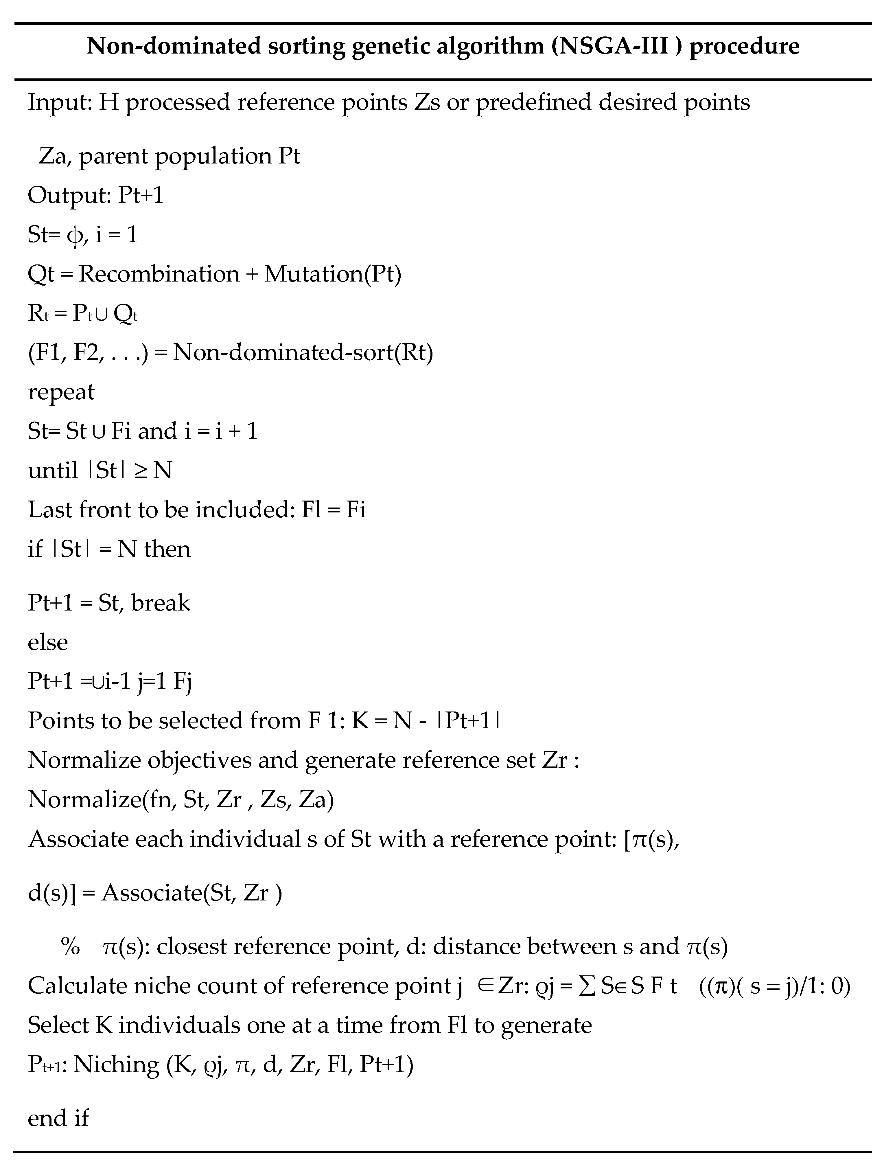
4.2. Non-Dominated Sorting Genetic Algorithm (NSGA-III)

A modified version of NSGA, called NSGA-II, developed by Deb et al. (2000) and Deb et al. (2002), utilizes a fast non-dominated sorting genetic algorithm. This method is computationally efficient, non-elitism preventing, and less dependent on a sharing parameter for diversity preservation. Recently, a reference-point based multi-objective NSGA-II algorithm (called NSGA-III) is proposed by Deb and Jain, which is more efficient to solve problems with more than two objectives [33]. The main procedure of NSGA-III can be briefly described below. NSGA-III starts with the definition of a set of reference points. Then an initial population with N members is randomly generated, where N is the population size. The next steps are iterated until the termination criterion is satisfied. At the t-th generation, the current parent population Pt is used to produce an offspring population Q_t by using random selection, simulated binary crossover (SBX) operator and polynomial mutation. The size of Pt and Qt are both N. subsequently, the two populations P_t and Q_t are merged together to form a new population R_t = P_t∪Q_t (of size 2N). To choose the best N members from R_t for the next generation, the non-dominated sorting based on the usual domination principle [34,35] is first used, which classifies R_t into different non-domination levels (F₁, F₂, and so on). Then, a new population S_t is constructed by filling members of different non-domination levels one at a time, starting from F₁, until the size of St equals to N or for the first time becomes greater than N. Let us suppose that the last level included is the l-th level. Hence, the solutions from the level l + 1 onwards are simply rejected. Members in S_t\F_l are already chosen for P_t+1, and the remaining population slots are chosen from F_l such that the desired diversity is maintained in the population. In the original NSGA-II, the solutions in F_l with the largest crowding distance values are selected. However, the crowding distance measure does not perform well for many-objective problems. Thus, the selection mechanism in NSGA-III is modified by conducting a more systematic analysis of members in S_t with respect to the supplied reference points. To achieve this, objective values and supplied reference points are first normalized so that they have an identical range. After normalization, the ideal point of the set S_t is the zero vectors. Thereafter, the perpendicular distance between a member in St and each of the reference lines (joining the ideal point with a reference point) is calculated. Each member in S_t is then associated with a reference point having the minimum perpendicular distance. Next, the niche count ρj for the j-th reference point, defined as the number of members in S_t\F_l that are associated with the j-th reference point, can be obtained based on the above process. Further, a niche-preservation operation is executed to select members from Fl, and it works as follows. First, the reference point set J_min = {j:argmin_j$\rho$_j} having the minimum $\rho$_j value is identified. In case of |J_min| > 1, one ¯j $\in$ J_min is randomly chosen. If $\rho$¯_j = 0, we choose the one having the shortest perpendicular distance to the j-th reference line among members associated with the j-th reference point in F_l and add it to P_t+1. The count of $\rho$¯_j is then increased by one. In the event $\rho$_j ≥ 1, a randomly chosen member from front Fl that is associated with the j-th reference point is added to P_t+1, and the count of $\rho$¯_j also needs increasing by one. In both of the two cases, once there exists no such member to be selected, the j-th reference point is excluded from further consideration for the current generation. After niche counts are updated, the above niche operation is repeated for a total of K = N − |S_t \ F_l| times to fill the remaining population slots of P_t+1. For more details of NSGA-III, please refer to [33].The pseudo-codes of NSGA-III are shown in Figure 1.

4.3. Best Compromise Solution

The power system operators may have imprecise goals for the DERs planning problem. Therefore, a fuzzy-based mechanism is employed over the tradeoff curve of the Pareto optimal set obtained by the MOWCA and NSGA-III algorithm to extract the best compromise solution. The value of the membership function ${\mathsf{\mu }}_{\mathrm{i}}^{\mathrm{k}}$ is calculated for the $\mathrm{k}$th solution of the $\mathrm{i}$th objective function, as follows [34]:

$${\mathsf{\mu }}_{\mathrm{i}}^{\mathrm{k}}=\left\{\begin{array}{c}1 \mathrm{for} {\mathrm{F}}_{\mathrm{i}}\left(\mathrm{x}\right)\le {\mathrm{F}}_{\mathrm{i}}^{\min }\\ \frac{{\mathrm{F}}_{\mathrm{i}}^{\mathrm{Max}}-{\mathrm{f}}_{\mathrm{i}}\left(\mathrm{x}\right)}{{\mathrm{F}}_{\mathrm{i}}^{\mathrm{Max}}-{\mathrm{F}}_{\mathrm{i}}^{\mathrm{Min}}} \mathrm{for} {\mathrm{F}}_{\mathrm{i}}^{\mathrm{Min}}\le {\mathrm{f}}_{\mathrm{i}}\left(\mathrm{x}\right)\le {\mathrm{F}}_{\mathrm{i}}^{\mathrm{Max}}\\ 0 \mathrm{for} {\mathrm{F}}_{\mathrm{i}}\left(\mathrm{x}\right)\ge {\mathrm{F}}_{\mathrm{i}}^{\max }\end{array}\right.$$

(43)

For each non-dominated solution in the archive set, the normalized membership function ${\mathrm{U}}^{\mathrm{k}}$ is calculated as follows:

$${\mathrm{U}}^{\mathrm{k}}=\frac{{{\displaystyle \sum }}_{\mathrm{i}=1}^{{\mathrm{N}}_{\mathrm{obj}}}{\mathsf{\mu }}_{\mathrm{i}}^{\mathrm{k}}}{{{\displaystyle \sum }}_{\mathrm{k}=1}^{{\mathrm{N}}_{\mathrm{Archive}}}{{\displaystyle \sum }}_{\mathrm{i}=1}^{{\mathrm{N}}_{\mathrm{obj}}}{\mathsf{\mu }}_{\mathrm{i}}^{\mathrm{k}}}$$

(44)

The solution that has the maximum value of ${ \mathrm{U}}^{\mathrm{k}}$ is considered the best compromise solution. In this paper, all objective functions have the same importance (weight factor).

The values of input data parameters used in NSGA-III and MOWCA are summarized in

Table 4. Values of parameter settings used in non-dominated sorting genetic algorithm (NSGA-III) and multi-objective water cycle algorithm (MOWCA).

Parameter	NSGA-III	Parameter	MOWCA
Population size N	80	Population size	80
Evaluation generation	50	Evaluation generation	50
Crossover probability (pc)	0.5	Nsr (Number of rivers + sea)	4
Mutation probability (pm)	0.5	dmax (Maximum allowable distance between river and sea)	1×10−16
Distribution index for a crossover (ηc)	30
Distribution index for mutation (ηm)	20

.

5. Results and Discussion

To define the impact of the suggested algorithm carried out on a test system of IEEE-33 bus systems and the IEEE-69 bus network. The cost of the energy losses per kWh is supposed to be $0.05 [31]. The planning of hybrid power system model added to different load models, like constant, residential and commercial load models at summer day load (SDM) and winter day load (WDM) are made by employing MOWCA and NSGA-III form minimization of total power loss, total annual energy cost, and emission while placing the DERs in appropriate locations. The simulations have been carried out over six different cases as shown in

Table 5. The case studies presented in this study.

Case Study	Load Models		System
Case 1	Constant load		IEEE- 33 bus system
Case 2	Residential load Commercial load	At summer day
Case 3	Residential load Commercial load	At winter day
Case4	Constant load		IEEE-69 bus system
Case5	Residential load Commercial load	At summer day
Case 6	Residential load Commercial load	At winter day

.

5.1. IEEE 33- Bus System

For examining the feasibility of the suggested MOWCA optimization technique, a test system consists of 33-bus and 32 branches are used. 100 MVA, and 12.66 kV operating parameters, and loading parameters are 3720 kW and 2300 kVAr respectively. The active and reactive losses without installing DER units are 202.7 kW and 140.03 kVAr, respectively. The system parameters are found in [31].

5.1.1. Case 1: Constant Load Model

The results calculated by the suggested MOWCA algorithm are shown in Table 4. It is compared to the results obtained by other techniques like NSGA-III for comparative study with the suggested algorithm. It is observed from

Table 6. Simulation results using MOWCA and NSGA-III for optimization of power loss, annual economic loss and emission under different loads such as the Summer Day Load Model (SDM) and Winter Day Load Model (WDM) (IEEE-33 bus systems).

Method	Type of DG	Constant		Summer Day Load Model (SDM)						Winter Day Load Model (WDM)
				Residential Load			Commercial Load			Residential Load			Commercial Load
		Location (bus no)	Size (kW)	Location (bus no)		Size (kW)	Location (bus no)		Size (kW)	Location (bus no)		Size (kW)	Location (bus no)	Size (kW)
MOWCA method	MT	(27) (13) (13)	89.751 73.116 0	(13) (26) (27)		135.25 150 129.85	(9) (5) (24)		250 172.95 100	(6) (9) (19)	198.37 121.99 153.42		(32) (27) (27)	241.53 116.8 0
	FC	(19) (13) (29)	205.74 0 210.71	(16) (6) (27)		137.14 186.18 0	(5) (10) (18)		0 323.36 400	(19) (11) (24)	0 152.96 191.82		(4) (24) (20)	146.76 220.32 200
	PV	(18) (14) (26)	-	(21) (28) (14)		-	(30) (8) (28)		-	(15) (10) (22)	-		(13) (8) (30)	-
	WT	(16) (28) (8)	-	(24) (29) (12)		-	(32) (6) (29)		-	(14) (26) (16)	-		(17) (23) (15)	-
	F1 (kW)	103.9202		71.2596			54.95523			69.68398			59.18302
	F2 ($)	683.595.915		710.536.85			793,960.79887			738.466.285			835.280.76
	F3 (Ib/h)	5489.94691		5105.50415			4779.93565			4928.2749			4624.96045
NSGA-III method	MT	(31) (32) (23)	58.58 247 134.5	(27) (5) (9)	2.161 59.053 116.97		(21) (17) (2)	0.23526 0.021001 0.032842		(33) (28) (11)	223.4 101.4 175.99		(17) (11) (18)		19.834 242.84 133.4
	FC	(7) (7) (25)	17.24 0343.6	(14) (18) (14)	218.51 324.28 0		(17) (33) (15)	0 0.33302 0.12261		(21) (15) (9)	109.5 162.5 191.4		(11) (12) (23)		0 229.63 251.36
	PV	(4) (15) (12)	-	(22) (16) (30)	-		(18) (14) (19)	-		(25) (26) (31)	-		(3) (27) (31)		-
	WT	(12) (28) (17)	-	(12) (2) (32)	-		(4) (30) (25)	-		(31) (6) (28)	-		(21) (24) (14)		-
	F1(kW)	96.54708		77.65119			70.53227			53.64945			64.16248
	F2 ($)	744204.37		757584.55805			739478.40639			818483.8614			792.522.977
	F3(Ib/h)	5520.95828		5078.22182			4964.23913			5087.94170			4793.43071

* The best solution marked in bold.

that a significant reduction is achieved by MOWCA in the annual energy cost (683,595.915 $) and Emission (5489.94691 Ib/h) in comparison with NSGA-III while the power loss achieved by MOWCA method (103.9202 kW) is higher than NSGA-III method. Figure 2 shows a set of non-dominated solutions or Pareto optimal fronts of constant load model.

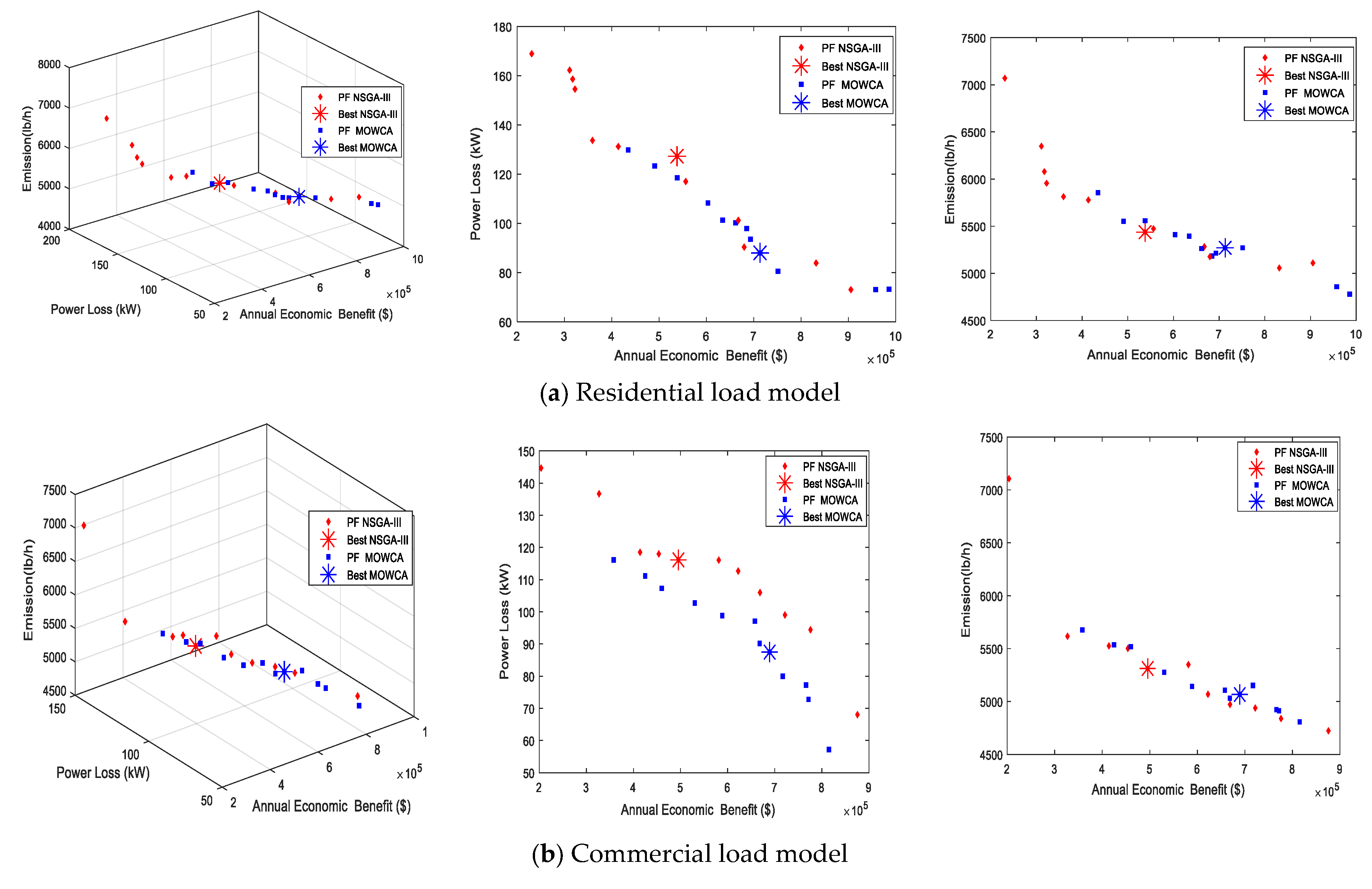
5.1.2. Case 2: Summer Day Load Model (SDM)

• Residential load

Table 6 depicts the multi-objective output for the residential load model. The network losses are 164kW before the installation of any DER, and after installing they are reduced to 71.2596 kW.From Table 4 it is clear that the MOWCA method significantly improves the system performance in terms of reduction of the power loss of (71.2596kW) and annual energy cost (710,536.85$)as compared with NSGA-III. However, the emission (5078.22182Ib/h) is less in NSGA-III.

• Commercial load

Table 6 illustrates the obtained results from implementing multi-objective optimization for the commercial load model. Before installing any DER the system losses are 152 kW and after installing they are reduced to 54.95 kW. The simulation results show that the MOWCA method reduces power losses and emissions. However, the annual energy cost is less in NSGA-III. Figure 3 shows Pareto optimal fronts and three dimensional residential and commercial load models at summer day load model.

5.1.3. Case 3: Winter Day Load Model (WDM)

• Residential load

The output results using MOWCA optimization algorithms are compared to the NSGA-III method and summarized in Table 6. The comparison proves that the suggested MOWCA provides the most reduction is achieved in annual cost and emission as compared with NSGA-III method. While the power loss achieved by MOWCA (69.68398 kW) is higher than NSGA-III (53.64945 kW).

• Commercial load

The output results deduced using the suggested MOWCA are compared to NSGA-III as presented in Table 6. It may be notified that MOWCA significantly reduces the power loss and emission as compared with the NSGA-III algorithm. However, the annual cost is less in NSGA-III. Figure 4 shows Pareto optimal fronts and three dimensional residential and commercial load models at the winter day load model.

5.2. IEEE 69- Bus System

To show the performance of the proposed optimization techniques on a huge network is developed using a 69-bus network, the second test system used is 69-bus systems with a load of 3800 kW and 2690 kVAr, respectively and the data related to this test system was taken from [31]. Before the placement of DG units, the total active and reactive power losses are 224.95 kW and 102.12 kVAr, respectively.

5.2.1. Case 4: Constant Load Model

From

Table 7. Simulation results using MOWCA and NSGA-III for optimization of power loss, annual economic loss and emission under different loads such as SDM and WDM (IEEE-69 bus systems).

Method	Type of DG	Constant			Summer Day Load Model(SDM)								Winter Day Load Model(WDM)
					Residential Load				Commercial Load				Residential Load							Commercial Load
		Location (bus no)		Size (kW)	Location (bus no)			Size (kW)	Location (bus no)			Size (kW)	Location (bus no)				Size (kW)		Location (bus no)		Size (kW)
Proposed MOWCA	MT	(6) (62) (45)	123.6 197.44 61.991		(45) (39) (37)		98.874 131 24.193		(54) (35) (59)		204.1 100.58 0.17812		(19) (15) (47)	187.33 75.74 149.42					(28) (53) (21)		164.19 30.188 85.132
	FC	(62) (20) (7)	0 136.72 302.2		(38) (62) (44)		50.602 392.54 173.06		(21) (61) (30)		216.05 274.91 65.198		(56) (60) (36)		2.3104 355.13 96.482				(24) (32) (55)		257.94 65.586 207.26
	PV	(24) (41) (65)	-		(15) (65) (68)		-		(7) (38) (11)		-		(63) (32) (33)		-				(64) (23) (67)		-
	WT	(15) (12) (44)	-		(20) (21) (5)		-		(27) (64) (53)		-		(41) (64) (31)		-				(62) (46) (31)		-
	F1 (kW)	135.852			88.02824				87.47904				78.90383						96.37189
	F2 ($)	653.778.637			713.190.23449				689.160.668				669.380.049						661.212.176
	F3 (Ib/h)	5622.082			5270.99823				5066.35384				5094.87203						4991.83448
NSGA-III method	MT	(55) (45) (33)	46.52 173.36 111.68		(50) (20) (6)	96.838 0 149.14			(37) (36) (46)	109.69 19.288 17.67			(37) (24) (51)			0 116.5 116.5			(43) (6) (43)			0 0 0
	FC	(11) (60) (54)	117.83 331.41 184.07		(50) (19) (31)	0 201.44 147.54			(52) (52) (29)	75.316 0 262.41			(26) (26) (33)			296.54 0 0			(40) (500) (28)			0 300 0
	PV	(51) (15) (40)	-		(23) (24) (60)	-			(62) (51) (33)	-			(65) (21) (35)			-		(33) (47) (63)				-
	WT	(46) (38) (47)	-		(27) (34) (39)	-			(16) (54) (25)	-			(4) (7) (38)			-		(26) (18) (7)				-
	F1 (kW)	152.73747			127.309				116.14785				111.44034					120.86334
	F2 ($)	744.761.744			537.874.808				495.466.135				499.478.626					418.812.277
	F3 (Ib/h)	5498.66641			5437.09658				5311.83193				5473.49029					5411.5537

* The best solution marked in bold.

, it is clearly notified that the results obtained by MOWCA show that significant reduction is achieved in the active power losses (135.852 kW) and annual energy cost (653,778.637$) in comparison with NSGA-III while the emission achieved by MOWCA method (5622.082 Ib/h) is higher than NSGA-III method. A group of non-dominated solutions or Pareto optimal fronts of constant load model are shown in Figure 5.

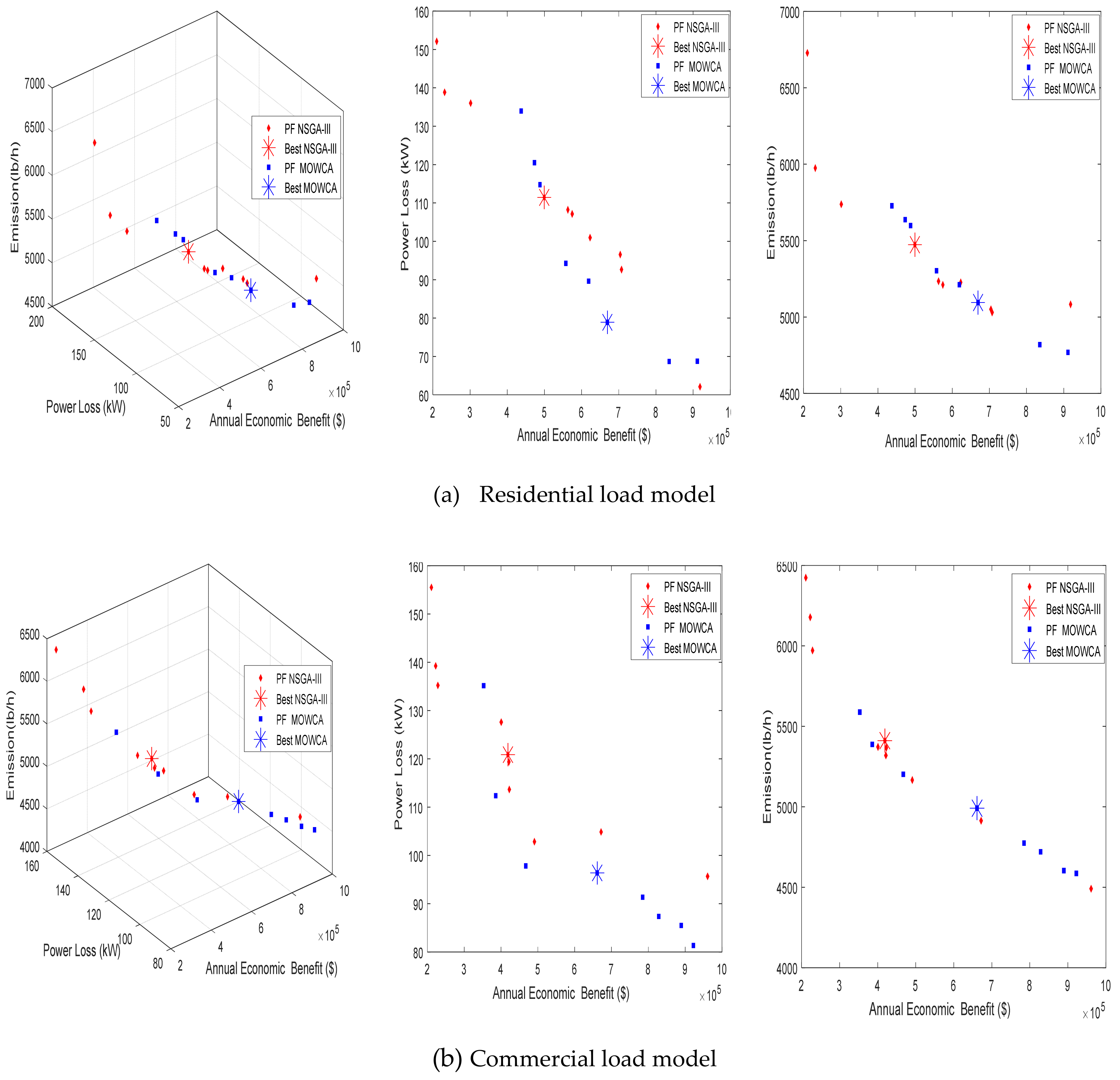
5.2.2. Case 5: Summer Day Load (SDM)

• Residential load

Before installing any DER the system losses are 177 kW active power loss and after installing they are reduced to 88.02824 kW. Form Table 7, it can be noticed that the results obtained by MOWCA show that significant reduction is achieved in power loss (88.02824 kW) and emission (5270.99823 Ib/h) as compared with the NSGA-III while the annual economic benefit achieved by MOWCA(713,190.234$) is higher than NSGA-III (537,874.808$).

• Commercial load

Before installing any DER, the system losses are 162 kW active power loss and after installing they are reduced to 97.75 kW. Form Table 7, it can be seen that the MOWCA method significantly improve the system performance in terms of reduction of power loss of (87.47904 kW) and emission (5066.35384 Ib/h) as compared with NSGA-III. However, the annual economic benefit is less in NSGA-III method. Figure 6 shows Pareto optimal fronts and three dimensional of residential and commercial load model at summer day load.

5.2.3. Case 6: Winter Day Load Model (WDM)

• Residential load

Without allocation DER, the network losses are 161 kW and after installing they are reduced to 78.90383 kW. The simulation results show that the MOWCA method reduces power losses and emission in an effective manner. However, the total annual energy cost is high compared with the method NSGA-III.

• Commercial load

Without installing DER, the network losses are 159 kW and after installing they are reduced to (96.37189 kW). It may further be noted from Table 7 that the power losses and emission obtained by the MOWCA method which provides highly accurate results in compared with that obtained by NSGA-III method while the annual energy cost achieved by NSGA-III is lower than MOWCA method. Figure 7 shows Pareto optimal fronts and three dimensional residential and commercial load models at winter day load.

6. Conclusions

In this article, the Multi-objective Water Cycle Algorithm (MOWCA) is proposed to determine the optimum placement and size of a hybrid power system model consisting of various combinations of a conventional system and renewable energy resources. Various optimization problems are addressed in this article such as real power loss, annual energy cost, and greenhouse gas emission as objective functions. The prime aim of considering these objectives is minimization of power loss, annual energy cost, and greenhouse gas emission. The DER planning with MOWCA method is tested for different voltage-dependent load models, namely constant, residential, and commercial load at summer and winter day load models in IEEE 33 bus and 69 bus distribution systems. The attained results by MOWCA method are compared with NSGA-II algorithm to validate its performance. It is clear from the comparison of simulation results that MOWCA was capable of obtaining better solutions than NSGA-III approach for multi-objective problems. The results indicated that enhancement of the distribution power system performance parameters depends on the size of DERs and their suitable placement in the distribution power systems. It was clear the proposed MOWCA method proves that the economic and environmental benefit is achieved with the optimal allocation of DERs at the constant load and residential load in the winter day load model regarding to other load models for IEEE 33-bus system while technical and economic benefit is got at the constant load with respect to other load models for the IEEE 69-bus system. The technical and environmental benefit is obtained at commercial load in summer and winter day load model for the IEEE 33-bus system and also at residential load for the IEEE 69-bus system while the technical and e economic benefit is attained at residential load in summer day load model for IEEE 33-bus system.

References

1. Sawle, Y.; Gupta, S.C.; Bohre, A.K. Review of hybrid renewable energy systems with comparative analysis of off-grid hybrid system. Renew. Sustain. Energy Rev. 2018, 81, 2217–2235. [Google Scholar] [CrossRef]
2. Zhang, W.; Maleki, A.; Rosen, M.A.; Liu, J. Optimization with a simulated annealing algorithm of a hybrid system for renewable energy including battery and hydrogen storage. Energy 2018, 163, 191–207. [Google Scholar] [CrossRef]
3. Diemuodeke, E.O.; Addo, A.; Oko, C.O.C.; Mulugetta, Y.; Ojapah, M.M. Optimal mapping of hybrid renewable energy systems for locations using multi-criteria decision-making algorithm. Renew. Energy 2019, 134, 461–477. [Google Scholar] [CrossRef]
4. Guo, S.; Liu, Q.; Sun, J.; Jin, H. A review on the utilization of hybrid renewable energy. Renew. Sustain. Energy Rev. 2018, 91, 1121–1147. [Google Scholar] [CrossRef]
5. Buch, H.; Trivedi, I.N. A new non-dominated sorting ions motion algorithm: Development and applications. Decis. Sci. Lett. 2019, 9, 59–76. [Google Scholar] [CrossRef]
6. Mirjalili, S.; Jangir, P.; Saremi, S. Multi-objective ant lion optimizer: A multi-objective optimization algorithm for solving engineering problems. Appl. Intell. 2017, 46, 79–95. [Google Scholar] [CrossRef]
7. Tawhid, M.A.; Savsani, V. Multi-objective sine-cosine algorithm (MO-SCA) for multi-objective engineering design problems. Neural Comput. Appl. 2019, 31, 915–929. [Google Scholar] [CrossRef]
8. Bhadoria, V.S.; Pal, N.S.; Shrivastava, V. Artificial immune system based approach for size and location optimization of distributed generation in distribution system. Int. J. Syst. Assur. Eng. Manag. 2019, 10, 339–349. [Google Scholar] [CrossRef]
9. Mobin, M.; Mousavi, S.M.; Komaki, M.; Tavana, M. A hybrid desirability function approach for tuning parameters in evolutionary optimization algorithms. Measurement 2018, 114, 417–427. [Google Scholar] [CrossRef]
10. Veeramani, C.; Sharanya, S. Analyzing the Performance Measures of Multi-Objective Water Cycle Algorithm for Multi-Objective Linear Fractional Programming Problem. In Proceedings of the 2018 Second International Conference on Intelligent Computing and Control Systems (ICICCS), Madurai, India, 14–15 June 2018; pp. 297–306. [Google Scholar]
11. Devabalaji, K.R.; Ravi, K. Optimal size and sitting of multiple DG and DSTATCOM in radial distribution system using Bacterial Foraging Optimization Algorithm. Ain Shams Eng. J. 2016, 7, 959–971. [Google Scholar] [CrossRef]
12. Melgar-Dominguez, O.D.; Pourakbari-Kasmaei, M.; Lehtonen, M.; Mantovani, J.R. Voltage-Dependent Load Model-Based Short-Term Distribution Network Planning Considering Carbon Tax Surplus. IET Gener. Transm. Distrib. 2019, 13, 3760–3770. [Google Scholar] [CrossRef]
13. Chauhan, A.; Saini, R.P. Discrete harmony search based size optimization of integrated renewable energy system for remote rural areas of Uttarakhand state in India. Renew. Energy 2016, 94, 587–604. [Google Scholar] [CrossRef]
14. Halabi, L.M.; Mekhilef, S.; Olatomiwa, L.; Hazelton, J. Performance analysis of hybrid PV/diesel/battery system using HOMER: A case study Sabah, Malaysia. EnergyConvers. Manag. 2017, 144, 322–339. [Google Scholar] [CrossRef]
15. Guangqian, D.; Bekhrad, K.; Azarikhah, P.; Maleki, A. A hybrid algorithm based optimization on modeling of grid independent biodiesel-based hybrid solar/wind systems. Renew. Energy 2018, 122, 551–560. [Google Scholar] [CrossRef]
16. Peng, W.; Maleki, A.; Rosen, M.A.; Azarikhah, P. Optimization of a hybrid system for solar-wind-based water desalination by reverse osmosis: Comparison of approaches. Desalination 2018, 442, 16–31. [Google Scholar] [CrossRef]
17. Singh, S.S.; Fernandez, E. Modeling, size optimization and sensitivity analysis of a remote hybrid renewable energy system. Energy 2018, 143, 719–731. [Google Scholar] [CrossRef]
18. Ikeda, S.; Takeda, A.; Ohmori, H. Optimal sizing of photovoltaic systems for loss minimization in distribution network. In Proceedings of the 2018 SICE International Symposium on Control Systems (SICE ISCS), Tokyo, Japan, 9–11 March 2018; pp. 185–192. [Google Scholar]
19. Nadjemi, O.; Nacer, T.; Hamidat, A.; Salhi, H. Optimal hybrid PV/wind energy system sizing: Application of cuckoo search algorithm for Algerian dairy farms. Renew. Sustain. Energy Rev. 2017, 70, 1352–1365. [Google Scholar] [CrossRef]
20. Samy, M.M.; Barakat, S.; Ramadan, H.S. A flower pollination optimization algorithm for an off-grid PV-Fuel cell hybrid renewable system. Int. J. Hydrog. Energy 2019, 44, 2141–2152. [Google Scholar] [CrossRef]
21. Duong, M.Q.; Pham, T.D.; Nguyen, T.T.; Doan, A.T.; Tran, H.V. Determination of Optimal Location and Sizing of Solar Photovoltaic Distribution Generation Units in Radial Distribution Systems. Energies 2019, 12, 174. [Google Scholar] [CrossRef]
22. Yahiaoui, A.; Benmansour, K.; Tadjine, M. Control, analysis and optimization of hybrid PV-Diesel-Battery systems for isolated rural city in Algeria. Sol. Energy 2016, 137, 1–10. [Google Scholar] [CrossRef]
23. Li, Y.; Feng, B.; Li, G.; Qi, J.; Zhao, D.; Mu, Y. Optimal distributed generation planning in active distribution networks considering integration of energy storage. Appl. Energy 2018, 210, 1073–1081. [Google Scholar] [CrossRef]
24. Asmi, R.Y.; Salama, M.; Ahmad, I.A. Distributed generation’s integration planning involving growth load models by means of genetic algorithm. Arch. Electr. Energy 2018, 67, 667–682. [Google Scholar]
25. Singh, B.; Mukherjee, V.; Tiwari, P. GA-based multi-objective optimization for distributed generations planning with DLMs in distribution power systems. J. Electr. Syst. Inf. Technol. 2017, 4, 62–94. [Google Scholar] [CrossRef]
26. Moradi, M.H.; Eskandari, M.; Hosseinian, S.M. Operational strategy optimization in an optimal sized smart micro grid. IEEE Trans. Smart Grid 2015, 6, 1087–1095. [Google Scholar] [CrossRef]
27. Aghajani, G.R.; Shayanfar, H.A.; Shayeghi, H. Demand side management in a smart micro-grid in the presence of renewable generation and demand response. Energy 2017, 126, 622–637. [Google Scholar] [CrossRef]
28. Esmaeili, M.; Sedighizadeh, M.; Esmaili, M. Multi-objective optimal reconfiguration and DG (Distributed Generation) power allocation in distribution networks using Big Bang-Big Crunch algorithm considering load uncertainty. Energy 2016, 103, 86–99. [Google Scholar]
29. Aien, M.; Hajebrahimi, A.; Fotuhi-Firuzabad, M. A comprehensive review on uncertainty modeling techniques in power system studies. Renew. Sustain. Energy Rev. 2016, 57, 1077–1089. [Google Scholar] [CrossRef]
30. Imran, M.; Kowsalya, M. Optimal size and siting of multiple distribution generators in distribution system using bacterial foraging optimization. Swarm Evol. Comput. 2014, 15, 58–65. [Google Scholar] [CrossRef]
31. Kefayat, M.; Ara, A.L.; Niaki, S.N. A hybrid of ant colony optimization and artificial bee colony algorithm for probabilistic optimal placement and sizing of distributed energy resources. Energy Convers. Manag. 2015, 92, 149–161. [Google Scholar] [CrossRef]
32. Rao, B.H.; Sivanagaraju, S. Optimum allocation and sizing of distributed generations based on clonal selection algorithm for loss reduction and technical benefit of energy savings. In Proceedings of the 2012 International Conference on Advances in Power Conversion and Energy Technologies (APCET), Mylavaram, Andhra Pradesh, India, 2–4 August 2012; pp. 1–5. [Google Scholar]
33. Sadollah, A.; Eskandar, H.; Kim, J.H. Water cycle algorithm for solving constrained multi-objective optimization problems. Appl. Soft Comput. 2015, 27, 279–298. [Google Scholar] [CrossRef]
34. Deb, K.; Jain, H. An evolutionary many-objective optimization algorithm using reference-point-based non-dominated sorting approach, part I: Solving problems with boxconstraints. IEEE Trans. Evol. Comput. 2014, 18, 577–601. [Google Scholar] [CrossRef]
35. Hashim, H.A.; Abido, M.A. Location management in lte networks using multi-objective particle swarm optimization. Comput. Netw. 2019, 157, 78–88. [Google Scholar] [CrossRef] [Green Version]
Figure 1. Non-dominated sorting genetic algorithm (NSGA-III).
Sustainability 11 06550 g001
Figure 2. Distribution of Pareto-optimal solution for the constant load model in the IEEE 33 bus system.
Sustainability 11 06550 g002
Figure 3. Distribution of Pareto-optimal solutions for residential and commercial load models at summer day load in the IEEE 33 bus system.
Sustainability 11 06550 g003
Figure 4. Distribution of Pareto-optimal solutions for residential and commercial load models at winter day load in the IEEE 33 bus system.
Sustainability 11 06550 g004
Figure 5. Distribution of Pareto-optimal solution for the constant load model in the IEEE 69 bus system.
Sustainability 11 06550 g005
Figure 6. Distribution of Pareto-optimal solutions for residential and commercial load models at summer day load in the IEEE-69 bus system.
Sustainability 11 06550 g006
Figure 7. Distribution of Pareto-optimal solutions for residential and commercial load models at winter day load in the IEEE-69 bus system.
Sustainability 11 06550 g007