Tramp Ship Routing and Scheduling with Speed Optimization Considering Carbon Emissions

Abstract

The International Maritime Organization (IMO) proposed to reduce the total CO₂ emissions of the maritime sector by 50% by 2050, and strive to gradually achieve the zero-carbon target. Therefore, shipping companies need to consider environmental impacts while pursuing benefits. In view of the tramp ship scheduling with speed optimization problem, considering carbon emissions, the configuration of owner ships and charter ships, and the impact of sailing speed on ship scheduling with the target of minimizing the total costs of shipping companies, multi-type tramp ship scheduling and speed optimization considering carbon emissions is established. A genetic simulated annealing algorithm based on a variable neighborhood search is proposed to solve the problem. Firstly, the ship type is matched with the cargo. Then the route is generated according to the time constraint, and finally, the neighborhood search strategy is adopted to improve the solution quality. The effectiveness of the proposed model and algorithm is verified by an example, which also confirms that ship scheduling and sailing speed joint optimization can reduce costs and carbon emissions. Research results can not only deepen the study of the theory of tramp scheduling but also to effectively solve the tramp shipping schedule considering carbon emissions problems faced by companies to provide theoretical guidance.

1. Introduction

Seaborne transportation is one of the main freight transportation modes and the only cost-effective option for transportation of large volumes between the continents. Within commercial shipping it is common to distinguish between three different basic operating modes: liner, tramp, and industrial. In contrast to liner shipping, tramp shipping does not consider service frequency. A ship can sail at different speeds on different sailing legs of a route. Compared with liner shipping, tramp ships have more research gaps and complexities.

The excessive emissions of greenhouse gases (GHG) increasingly intensify global climate warming, which not only jeopardizes the balance of natural ecosystems but also threatens the food supply and living environment of human beings. At the same time, with the rapid growth of world maritime trade volume, Maritime carbon dioxide emissions are projected to increase significantly in the coming decades. According to the International Maritime Organization (IMO), CO₂ emissions from the maritime sector in 2007 increased by 86% compared to 1990 and accounted for 3.3% of the world’s total emissions. This study’s BAU scenarios project an increase of 50% to 250% in the period to 2050 [1,2].

Sailing speed is an important factor considered by a shipping company because it has a significant impact on tramp ship routing and scheduling, including ship fuel cost. On one hand, a cubic function can describe the relationship between fuel consumption and speed. On the other hand, the sailing speed can also decide the sailing time of a ship route and affect ship carriers’ service quality as well as the shipper’s satisfaction. To ensure the cargo transported to the destination within the time window, meet the demand of the shipper, and obtain more profit, shipping companies need, therefore, to optimize the configuration of ships and their speeds, considering sailing speed optimization in tramp shipping has always been a concern of shipping companies.

At the same time, speed determines the sailing time and indirectly affects the amount of carbon dioxide emissions in the process of transportation. Therefore, it is an important issue to investigate optimizing sailing speed in order to reduce fuel costs and CO₂ emissions.

While considering the profits of shipping companies, it is necessary to pay attention to sustainability challenges such as air pollution, resource shortages, and human health problems. Strengthening energy conservation and reducing CO₂ emissions by ships will become an inevitable choice to alleviate the environmental pressure of sustainable development.

The main contribution of this paper is the proposed load dependent fuel consumption. In terms of modeling, it is the first to join the tramp ship routing and speed problem while considering carbon emissions. At the same time, we focus on a fleet of heterogeneous ships that is composed of owner ships and charter ships. We establish a nonlinear programming model and propose a variable neighborhood genetic simulated annealing (VNGSA) algorithm for this problem. Finally, we show that incorporating variable speeds in ship routing and scheduling can yield significant improvements in profits for the shipping company. Different objective functions will generally produce different solutions to the same problem, at the same time considering that carbon emissions can influence results in the choice of ship routing and cost.

The rest of this paper is organized as follows. Section 2 presents the literature review. In Section 3, we discuss modeling approaches for this class of problems, including problem descriptions and, assumptions. The VNGSA algorithm is described in Section 4. In Section 5, we evaluate the applicability of the proposed models and the efficiency of the algorithm. Finally, in Section 6, we present the paper’s conclusions.

2. Literature Review

The literature is summarized in three aspects: (1) tramp ship routing and scheduling models and methods, (2) speed optimization, and (3) carbon emissions consideration.

2.1. Tramp Ship Routing and Scheduling Models and Methods

In recent years, scholars have conducted an in-depth exploration of the problem of tramp ship routing and scheduling. Thai [3] proposed and validated a service quality (SQ) model for tramp shipping. Here, service quality was a key consideration by them. Armas [4] focused on the ship routing and scheduling problem with discretized time windows and proposed a hybridization of a greedy randomized adaptive search procedure and a variable neighborhood search (GRASP–VNS). Hennig [5] considered the crude oil tanker routing and scheduling problem with split pickup and split delivery and proposed two approaches to solve this problem. The discrete split model provides quicker results but lower quality solutions. The arbitrary split model provides better results but cannot solve large instances. One characteristic of the problem was that, in contrast to the problem discussed above, each ship was capable to carry several different products simultaneously in separate cargo tanks. Lee [6] solved an industrial ship routing problem of heterogeneous ships. They considered owner ships and tramp ships for industrial ship routing problem. An adaptive large neighborhood search-based heuristic was proposed. Hemmati et al. [7] presented a benchmark suite for ship routing and scheduling problems from industrial and tramp shipping. They proposed an adaptive large neighborhood search (ALNS) for solving the problem, which was used to provide best known results for the benchmark instances. Otherwise, a vendor managed inventory (VMI) service in tramp shipping was considered by Hemmati [8]. A two-phase heuristic was proposed to determine routing and scheduling for the shipping company and showed the influence of benefits obtainable through VMI. Siddiqui [9] presented a mixed-integer bi-objective optimization program to solve routing and scheduling of crude oil tankers from a cost and risk perspective. The conclusion was that larger vessels should be used if risk was more important. Wu [10] developed a two-step solution scheme, consisting of a dynamic programming algorithm and a tailored benders decomposition method to solve a stochastic backhaul cargo, canvassing problem for an industrial company that managed a fleet of bulk ships.

2.2. Speed Optimization

Speed optimization for ship routing and scheduling has attracted some attention recently. We have encountered several papers that address tramp ship routing and scheduling with speed. Norstad [11] and Hvattum [12] presented a multi-start local and an exact algorithm for the ship speed optimization problem with giving a fixed sequence of port calls, respectively. It was demonstrated that incorporating sailing speed as a decision variable when planning vessel routes significantly improved fleet utilization and profit. Meng [13] considered speed optimization, as the above did. However, he dealt with the jointing tramp ship routing and bunkering (JSRB) problem, which considering different bunker prices at different ports. The branch-and-price (B&P) approach incorporated an efficient method for obtaining the optimal bunkering policy. De [14] also addressed bunker fuel management strategies with shipping operations, it was different from the problem discussed above that provide adequate recovery policies for countering disruption within maritime transportation about container shipping. In 2019, De [15] also proposed an algorithm which was hybridizing basic variable neighborhood search with particle swarm optimization to solve sustainable ship routing and bunker management problem. Most of the research work pertaining to tramp ship routing only considered the combination transportation cost and port cost as the main objective function such as Li [16] and Li [17]. Li [16] studied the influence of different fuel consumption of semi-submersible vessels with full-load and no-load on heavy cargo distribution and optimal speed. The results of an application example show that compared with the traditional recursive smoothing algorithm (RSA), the global search method could reduce the transportation cost. Li [17] solved the problem of speed optimization by giving a fixed sequence of port calls. Wen investigated a combined full-shipload tramp ship routing and speed optimization, the objective of which was to determine which orders to serve and to find the optimal route for each ship and the optimal sailing speed on each leg of the route so that the total profit was maximized. A heuristic branch-and-price algorithm was proposed [18]. However, the port cost was no consideration in this paper. Due to the influence of demurrage and dispatch on the profit of the ship owner, Yu [19] established a speed optimization of tramp shipping considering probability of default and port choice. The two-stage particle swarm optimization algorithm (PSO) was used to solve the model. Through the experiment, demurrage and handling efficiency indicated that the profit of shipping companies would increase within a certain range with the increase of default rate, demurrage fee, and loading and unloading efficiency. Yet, they did not address the intricacies associated with carbon emissions in the tramp ship routing and scheduling domain.

2.3. Carbon Emissions Consideration

The fuel cost, and consequently CO₂ emissions, are strongly dependent on the sailing speed. With the development of greener shipping, Psaraftis [20] placed speed in the context of current developments and highlighted the role of ship speed in maritime transportation with respect to both economics and environment. At the same time, he surveyed models in the maritime transportation literature that embed ship speed as a decision variable and developed a taxonomy of these models according to several parameters. By investigating, Psaraftis [21] clarified some important issues as regards ship speed optimization at the operational level. In 2014, he incorporated the fuel price, freight rate, the inventory cost of the cargo, and the dependency of fuel consumption on the payload that weighs heavily in speed and routing decisions. Yet another study from sailing speed and environment was provided by Wang [22]. He established the sailing speed decision models under three different forms of carbon emission taxation. It turned out that considering the taxation of carbon emissions above a certain threshold was better than considering a model based on carbon emissions taxation. Wen [23], which investigated the routes and speeds optimized under time, cost, and environmental objectives, and a branch-and-price algorithm and a constraint programming model were developed. Computational experience with the algorithm was reported on a variety of objective functions. Yigit [24] focused on a new electrical energy management system and algorithm for the future ship and port designs. The influence of the system was proved by five cases, and the fundamental principles of the future ship and port designs for sustainable cities could be presented. Dere [25] investigated slow steaming from a novel perspective, and the cooling system was analyzed for decreased engine loads. The literature provided a few ship routing studies that were not focused on dynamic considerations. De [26] proposed Particle Swarm Optimization-Composite Particle (PSO-CP) to solve sustainable integrated dynamic ship routing and scheduling optimization. The complex problem incorporated several real-time constraints addressing the multiple time windows, varying supply and demand, carbon emission, etc. A small size numerical example was considered. To satisfy the demand at different ports during the planning horizon, De [27] incorporated sustainability aspects and several time window constraints. Owing to the inherent complexity of the aforementioned problem, an effective search heuristic was proposed. At the same time, De [28] considered different maritime operations, such as routing and scheduling of ships, time window concept considering port’s high tidal scenario, discrete planning horizon, carbon emission from the vessel, and ship’s draft restriction for maintaining the vessel’s safety at the port. His research addressed the sustainability and safety-related challenges associated with the complex, practical, and real-time maritime transportation problem. Different from this paper, De focused on port time window and port sustainability, while this paper focused on tramp ship routing and scheduling with speed optimization considering carbon emissions including a fleet of heterogeneous ships that was composed of owner ships and charter ships.

Most the work associated with tramp ship routing and scheduling fails to apprehend the importance of the fuel consumption of each ship depends individually on the sailing speed and the load of the ship. The earlier researches consider the fuel consumption only depends on the speed. In addition, it is absolutely clear that the earlier researches focused primarily on either ship routing or just speed and fuel consumption. They did not consider the joint optimization of speed and routing with carbon emissions. Most of the earlier researches did not care about a fleet of heterogeneous ships. In this paper, it proposed different modeling approaches for our problems than their formulations. Due to tramp ships having their particularity, the problem extends to the pickup and delivery problems with time windows (PDPTW) with a heterogeneous fleet, compatibility constraints, different ship starting points and starting times. The interplay of these complex attributes requires the joint optimization of multiple decision sets.

3. Problem Description and Mathematical Model

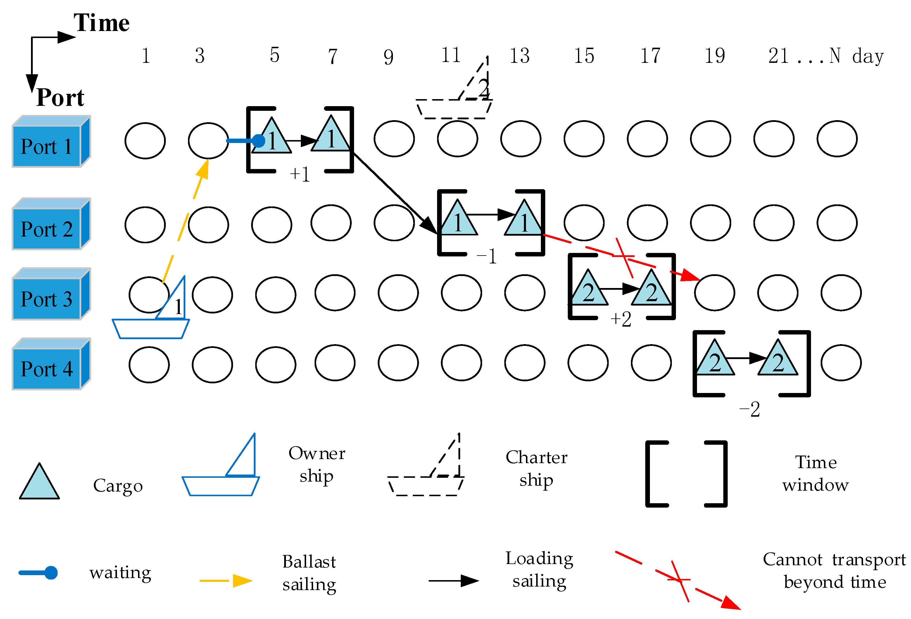
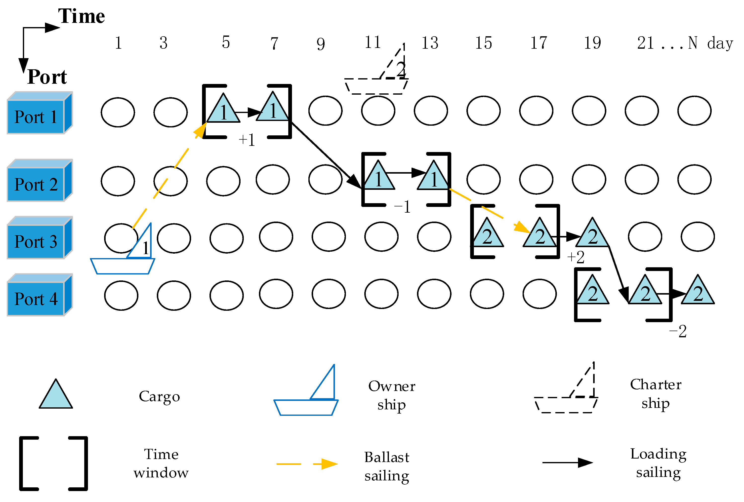
3.1. Problem Description

Consider a problem of tramp ship routing and scheduling with a fleet of heterogeneous ships. Assume that $n$ is the number of cargoes indexed by $i$. Associated with cargo $i$ is a loading port node $i$ and a discharging port node $n+i$. Let $N^P=\{1,2,3\dots n\}$ be the set of loading nodes and $N^D=\{n+1,n+2,n+3,\dots ,2n\}$ the set of delivery nodes. Note that several nodes can refer to the same physical port. The tramp ship routing and scheduling problem studied in this paper can be defined on a graph $(N^P\cup N^D,A)$, where $A=\{(i,j):i,j\in N^P\cup N^D,i\ne j\}$. Let $K=\{1,2\ne ,k,\ne \phi \}$ be the set of ships. The ship routing and scheduling with single speed is shown in Figure 1. The ship needs to wait at the port for the cargo 1. The cargo 2 cannot be transported by the owner ship, because ship 1 cannot arrive at port within the shipper’s desired time. Therefore, charter ship 2 will transport cargo 2.

Sailing speed has a significant impact on fuel cost and fuel consumption, as well as carbon emissions. Therefore, in order to reduce waiting time in the port and further reduce carbon emissions, ships can adopt a ‘slow-steaming’ strategy. Ship 1 can reduce its speed to arrive at port 1 within the desired time of the shippers and shorten the waiting time at the loading port of cargo 1. At the same time, the speed of the ship also determines the length of the sailing time. By adjusting the speed on the sailing leg from port 2 to port 3, the sailing time of ship 1 is changed from 6 days to 4 days, so ship 1 can arrive at the loading port of cargo 2 in time, as shown in Figure 2. Finally, ship routing and scheduling can reduce the number of charter ships. Thus, from the perspective of the shipping company, this paper not only focuses on improving the profit of the shipping company by optimizing the speed, but also takes into account the environment problem during transportation by considering the impact of carbon emissions, cargo, ports, and a fleet of heterogeneous ships on economic parameters comprehensively. We studied the optimal deployment of ships for a given transportation network. The main decision involves: formulating ship routing and scheduling and calculating the optimal speed, ship configuration, and carbon emissions strategy.

3.2. Model Assumptions

To facilitate the establishment of the model, the following assumptions are made:

(1)

The shipping company has a fleet of heterogeneous ships, which have their own attributes such as capacity, cruising speed, draft, and other parameters.

(2)

For transporting cargo, the shipping company is allowed to choose its owner ships or charter ships in the spot market.

(3)

Each cargo has a specific weight, loading port and discharging port, and time window. This information is known in advance. Cargoes cannot be split and should be picked up by exactly one ship during one visit. However, the ships are allowed to make multiple visits to a port if this is necessary.

(4)

Each ship is initially located at a given port and shall not return to the initial port after completing a voyage. A ship can sail at different speeds on different legs of the route as long as the speeds are within its feasible speed range.

(5)

Fuel price does not change over time.

3.3. Fuel Cost and Carbon Emissions Tax

Since heavy fuel is consumed during the sailing period, the daily fuel consumption of each ship (in tons/day) is given by a function $f(v,w)$ of the ship’s speed $v$ (in knots) and payload $w$ (in tons). In this paper, we use the realistic closed-form approximation of $f$ given in [23]:

$$f(v,w)=\mu v^3{(w+A)}^{2/3}$$

(1)

where $\mu$ is a constant, $v$ is the ship speed,$w$ is the payload, and $A$ is the ship of lightship weight.

Let $d_{ij}^{}$ be the sailing distance from node $i$ and $j$. Let variable $v_{ijk}$ be the sailing speed from node $i$ and $j$ with ship $k$. Let $p_{f1}$ be heavy fuel price. Therefore, heavy fuel consumption costs between nodes $i$ and $j$ for the ship is expressed as:

$$C_{ijk}^f=p_{f1}\mu v_{ijk}{}^3{(w_k+A_k)}^{2/3}\frac{d_{ij}}{24v_{ijk}}$$

(2)

Let $[E{T}_i,L{T}_i]$ denote the expected time window associated with node $i$. Let $t_{ik}$ denote the service time at node $i$ when visited by ship $k$. $T_{ik}$ is the time for arriving node $i$ for ship $k$. Let $C_{ik}^{pf}$ be the light fuel consumption of each ship in port. Since light fuel is consumed during berthing at port, the light fuel consumption during berthing at port can be demonstrated as:

$$C_{ik}^{pf}=\gamma [t_{ik}+((E{T}_i-T_{ik})\vee 0)]$$

(3)

where $\gamma$ represents light fuel consumption of the ship per hour at port (ton/h) and $\vee$ means that taking the lager of two.

$P_{ik}$ is lump-sum payment in port. Let $p_{f2}$ be the light fuel price and $C_{ik}^p$ denotes the port cost of node $i$ for owner ship $k$, including the lump-sum payment cost and light fuel consumption cost.

$$C_{ik}^p=P_{ik}+p_{f2}\gamma [t_{ik}+(E{T}_i-T_{ik})\vee 0]$$

(4)

$p_{c{o}_2}$ denotes carbon emissions tax rate, ${\epsilon }_1$ denotes carbon dioxide coefficient for heavy fuel, and ${\epsilon }_2$ denotes carbon dioxide coefficient for light fuel. Carbon emissions tax is obtained as:

$$C_{ijk}^{c{o}_2}=p_{c{o}_2}{\epsilon }_1\mu v_{ijk}{}^3{(w_k+A_k)}^{2/3}\frac{d_{ij}}{24v_{ijk}}+p_{c{o}_2}{\epsilon }_2\gamma [t_{ik}+(E{T}_i-T_{ik})\vee 0]$$

(5)

3.4. Notation Used in the Model

The graph $(N_k,A_k)$ is the sub-graph for ship $k$ in the model, and included in $N_k=N_k^P\cup N_k^D\cup o(k)\cup d(k)$ is the set of nodes that can be visited by ship $k$. We can extract the sets $N_k^P$ and $N_k^D$ consisting of the pickup and delivery nodes that ship $k$ may visit, respectively. $o(k)$ is the initial position for $k$, which could be in a port or sailing. $d(k)$ is an artificial destination node, which will be determined by the solution process and corresponds to the last delivery port for ship $k$. Let $q_i$ be the quantity of cargo $i$, while $Q_k$ represents the capacity of ship $k$. $C_i$ represents that node $i$ is transported by a spot charter. The interval $[v{b}_k^{\min },v{b}_k^{\max }]$ is ballast speed range for ship k. The interval $[v{l}_k^{\min },v{l}_k^{\max }]$ is loading speed range for ship $k$.

The variable $w_{ik}$ is the weight on board ship $k$ when leaving node $i$. The variable $x_{ijk}$ is equal to one if ship $k$ travels directly from node $i$ and $j$, and zero otherwise. The variable $Y_i$ is equal to one if node $i$ is transported by a charter ship in a spot market, and zero otherwise.

3.5. Mathematical Model

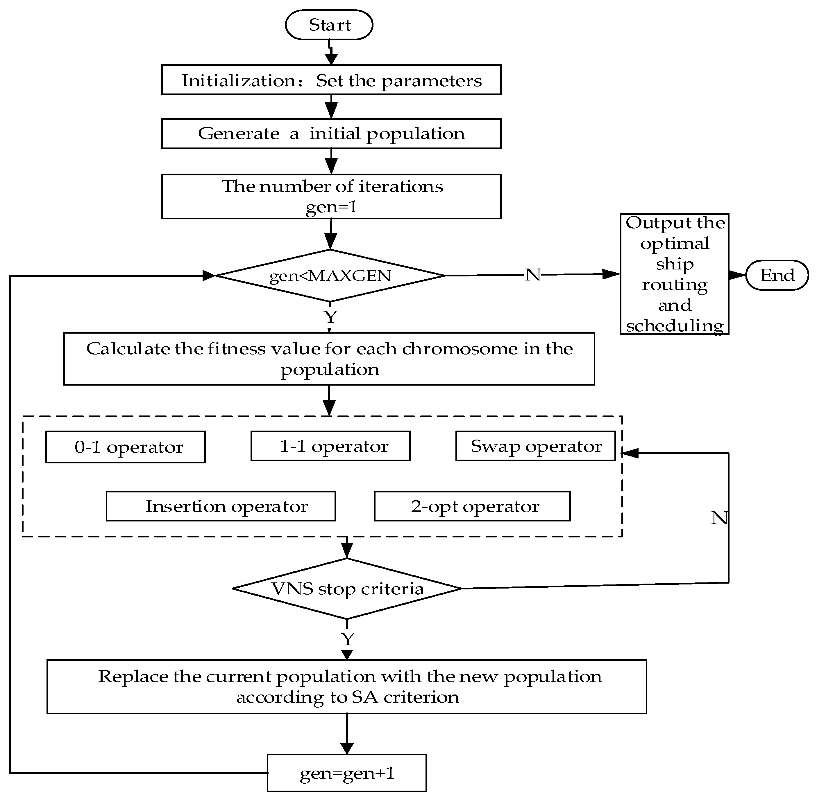
The model may be stated as follows:

$$\min {\displaystyle \sum _{k\in K}^{}{\displaystyle \sum _{(i,j)\in A_k}^{}{C}_{ijk}^f}}{x}_{ijk}+{\displaystyle \sum _{k\in K}^{}{\displaystyle \sum _{(i,j)\in A_k}^{}{C}_{ik}^p}}{x}_{ijk}+{\displaystyle \sum _{k\in K}^{}{\displaystyle \sum _{(i,j)\in A_k}^{}{C}_{ijk}^{c{o}_2}}}{x}_{ijk}+{\displaystyle \sum _{i\in N^P}^{}{C}_i}{Y}_i$$

(6)

The objective (6) minimizes the total cost of all the route legs, including fuel cost, port cost, CO₂ emissions cost, and charter cost.

$${\displaystyle \sum _{j\in N_k^P\cup \{d(k)\}}{x}_{o(k)jk}}=1\hspace{1em}\hspace{1em}\forall k\in K$$

(7)

$${\displaystyle \sum _{i\in N_k^D\cup \{o(k)\}}{x}_{id(k)k}}=1\hspace{1em}\hspace{1em}\forall k\in K$$

(8)

$${\displaystyle \sum _{j\in N_k}{x}_{ijk}}-{\displaystyle \sum _{j\in N_k}{x}_{jik}}=0\hspace{1em}\hspace{1em}\forall k\in K,i\in N_k\backslash \{o(k),d(k)\}$$

(9)

Constraints (7)–(9) describe the flow on the sailing route used by ship $k$.

$${\displaystyle \sum _{k\in K}{\displaystyle \sum _{j\in N_k}{x}_{ijk}}}+Y_i=1\hspace{1em}\hspace{1em}\hspace{1em}\forall k\in K,i\in N_{}^P$$

(10)

Constraint (10) states that all cargoes are transported, either by a ship in the fleet or by a spot charter ship.

$${\displaystyle \sum _{j\in N_k}{x}_{ijk}}-{\displaystyle \sum _{j\in N_k}{x}_{j(n+i)k}}=0\hspace{1em}\hspace{1em}\forall k\in K,i\in N_k^P$$

(11)

Constraint (11) is a so-called paring constraint and precedence constraint that forces pickup node $i$ to be visited before the corresponding delivery node $n+i$ by the same ship.

$$x_{ijk}=0\hspace{1em}\hspace{1em}\hspace{1em}\hspace{1em}\forall k\in K,i\in N_k^P,j\in N_k^P$$

(12)

$$x_{ijk}=0\hspace{1em}\hspace{1em}\hspace{1em}\hspace{1em}\forall k\in K,i\in N_k^D,j\in N_k^D$$

(13)

Constraints (12) and (13) ensure that the ship cannot continuously be called at two loading ports or two discharging ports, respectively.

$$T_{ik}\vee E{T}_i+t_{ik}+d_{i(n+i)}/v_{i(n+i)k}=T_{(n+i)k}\hspace{1em}\hspace{1em}\forall k\in K,(i,j)\in A_k$$

(14)

$$x_{ijk}(T_{ik}\vee E{T}_i+t_{ik}+d_{ij}/v_{ijk})=T_{jk}\hspace{1em}\hspace{1em}\forall k\in K,(i,j)\in A_k$$

(15)

$$T_{jk}\le L{T}_j\hspace{1em}\hspace{1em}\forall k\in K,j\in N_k$$

(16)

Precedence constraint (14) means that the discharging node for cargo must be visited after its loading node. Constraint (15) states the relationship between the time of starting service at a node j and the departure time from the previous node i. Constraint (16) defines the time window in which service must start.

$$x_{i(n+i)k}{w}_{(n+i)k}=0\hspace{1em}\hspace{1em}\forall k\in K,i\in N_k^P,(i,n+i)\in A_k$$

(17)

$$x_{(n+i)jk}(q_j-w_{jk})=0\hspace{1em}\hspace{1em}\forall k\in K,i,j\in N_k^P,(n+i,j)\in A_k$$

(18)

$$0\le w_{ik}\le Q_k\hspace{1em}\hspace{1em}\forall k\in K,i\in N_k^{}$$

(19)

Constraints (17) and (18) ensure transportation is a full-shipload by ships. Constraint (19) ensures that the load on board does not exceed the ship’s capacity.

$$v{b}_k^{\min }\le v_{ijk}\le v{b}_k^{\max }\hspace{1em}\hspace{1em}\forall k\in K,i\in N_k\backslash N_k^P,j\in N_k^P$$

(20)

$$v{l}_k^{\min }\le v_{i(n+i)k}\le v{l}_k^{\max }\hspace{1em}\hspace{1em}\forall k\in K,i\in N_k^P$$

(21)

Constraint (20) is the lower and upper bounds for the ballast speed variables. Constraint (21) is the lower and upper bounds for the loading speed variables.

$$Y_i\in \{0,1\}\hspace{1em}\hspace{1em}\forall i\in N^P$$

(22)

$$x_{ijk}\in \{0,1\}\hspace{1em}\hspace{1em}\forall k\in K,(i,j)\in A_k$$

(23)

Binary restrictions on the flow variables are given by constraints (22) and (23).

4. Solution Method

The model is a nonlinear programming model with a complex structure and composition, including 0–1 variable, continuous variable, equation, and inequality. The Genetic Algorithm (GA) is a global search heuristic approach according to the principles of evolutionary biology, based on the principle of ‘survival of the fittest’. However, the algorithm has a disadvantage in falling into local optima easily. The Variable Neighborhood Search (VNS) algorithm can systematically traverse different search spaces that are defined by different neighborhood structures in order to obtain various search strategies. Compared with the genetic algorithm, VNS has a strong ability for local search and search depth. The Simulated Annealing (SA) algorithm is a global optimization algorithm that converges to the global optimal solution with a probability of l, which has asymptotic convergence and parallelism. The combination of three algorithms can simultaneously start to conduct a local search and global optimization. In this paper, a genetic simulated annealing algorithm based on a variable neighborhood search is proposed to solve the problem. The process is shown in Figure 3.

4.1. Encoding and Initial Feasible Solution

Due to the nature of the problem, we chose real-number encoding, the length of the chromosome is the number of cargoes, the location of the gene on the chromosome is where the order of the ship service cargo is located. In order to obtain an initial solution, consider two constraints about ship capacity and time. The specific method is as follows: Firstly, judge ships that are compatible with cargo, where cargo is defined as the set of contracts to be performed by the corresponding ship. Secondly, select the first cargo of the route with the first ship in order to analyze whether it is possible to assign the cargo to the ship or not. If it is possible to assign the cargo to the ship, check if the next cargo meets the constraints and move this cargo from the set of other ships at the same time. Otherwise, select the next ship from the list and repeat the same procedure until all ships are tried. For example, the problem is composed of three owner ships and ten cargoes, indexed by real-number encoding. The 1-2-4-5-3-7-9-8-6-10 constitutes a chromosome. Ship 1 can transport cargo {3-5-9-10}, Ship 2 can transport {2-3-4-5-8-9-10} cargoes, and Ship 3 can transport {1-2-3-4-5-6-7-8-9-10}. Ship 1 cannot meet the time window of cargo 10 constraints after transporting cargo 9, the route is 3-5-9. At this time, remove cargo 3,5, and 9 that have been arranged for transportation from the initial route generated by ships 2 and 3, the initial route of ship 2 becomes {2-4-8-10}, and the initial route of ship 3 is {1-2-3-4-6-7-8-10}. Then check whether ship 2 meets the time window requirements of each cargo loading and discharging port, and then generate route {2-4-8-10} by ship 2. Delete the cargo that has been arranged to transport with ship 3, checking whether the route of ship 3 can meet the time window constraint. Finally, a ship route is determined based on the loading dates, discharging dates, origins, and destinations of the cargo assigned to that ship.

4.2. Calculate Fitness

In this paper, we attempt to minimize the total cost of a tramp shipping company. In other words, the function presented in Equation (6) is used to calculate the total cost. Search for the fitness value of the optimal individual in the contemporary population. If pop _ best < global _ best, record the ship routing corresponding to the individual in this generation. Otherwise, the optimal value of the individual in this generation will not be accepted.

4.3. Variable Neighborhood Search Strategy

VNS systematically changes different neighborhoods within a local search. The sequence is defined as follows: Exchange, Swap, Insertion, and 2-opt. This sequential selection is applied based on cardinality, which implies moving from relatively poor to richer neighborhood structures, and significantly increases the ability of the local search, and avoids falling into local optima. In order to improve the running efficiency and shorten the running time, this paper introduces adaptive evolutionary pressure, $p=\beta ·\exp (\frac{gen-MAXGEN}{MAXGEN})$, $\beta =0.1~1$. In the early stage of evolution, in order to ensure the diversity of the population, the adaptive evolutionary pressure is less, in the later stage of evolution, in order to improve the quality of the solution, the adaptive evolutionary pressure is great. This search strategy is used instead of the crossover and mutation of the traditional genetic algorithm. We start the neighborhood search based on the distance between ports, so as to significantly increase the possibilities of finding higher quality solutions.

(1)

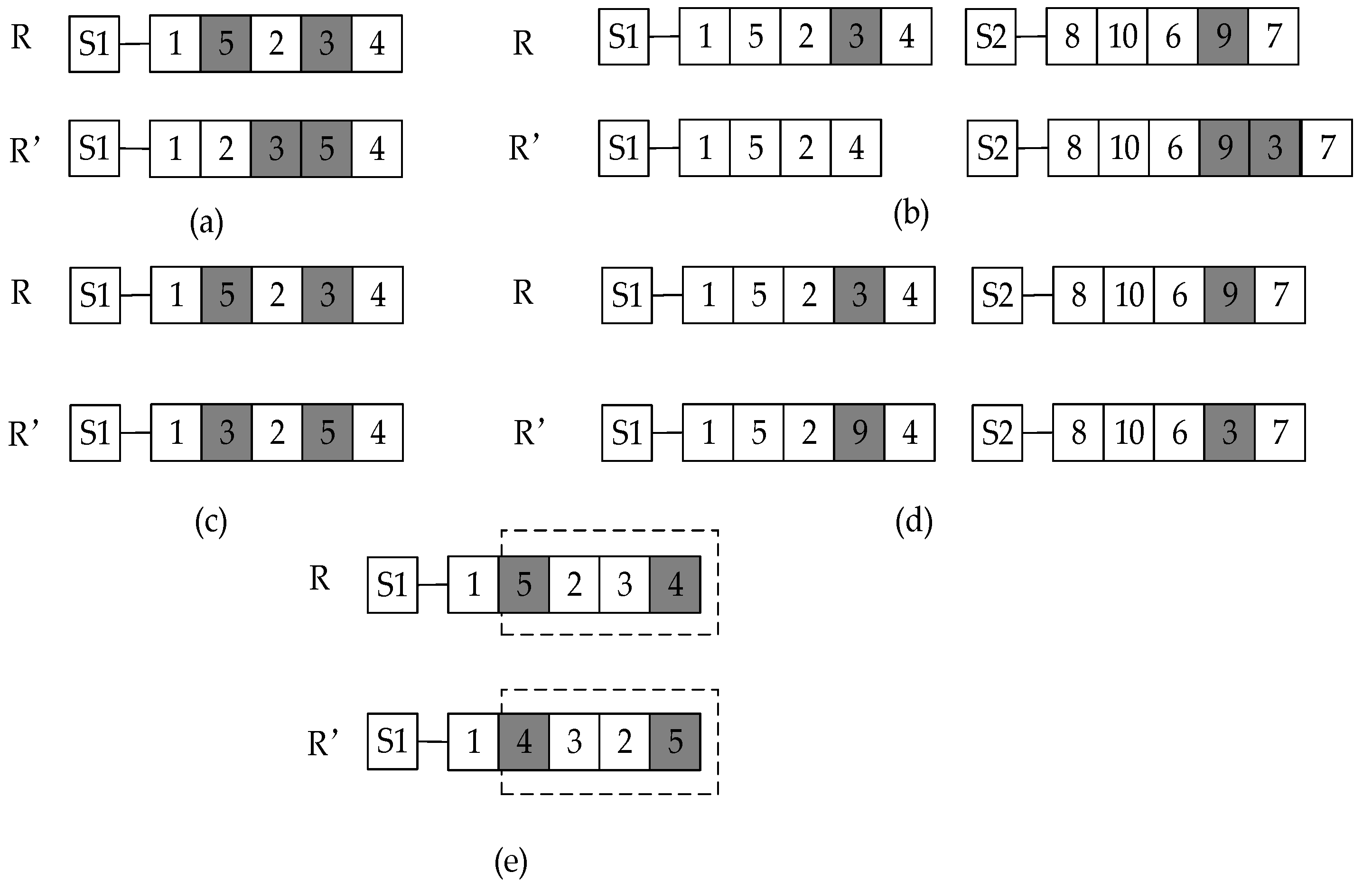
The 0–1 exchanged operator selects two points from a route randomly and tries to insert one point after the other point within the same route. Figure 4a shows an example where customer 5 and customer 3 are selected, we can insert customer 5 after customer 3 in R’.

(2)

The insertion operator chooses cargo $i$ from a route and $j$ from other routes randomly, deletes the cargo $i$ from a route, and inserts it into another route. Figure 4b shows an example where customer 3 on the S1 and customer 9 on the S2 are selected, we can insert customer 3 after customer 9 in R’.

(3)

The 1–1 exchanged operator selects two points from a route randomly and exchanges them. Figure 4c shows an example where customer 5 and customer 3 are selected, and we can relocate customer 5 and customer 3.

(4)

The swap operator selects a contract from a route, and another contract from another route, and swaps them. Figure 4d shows an example where customer 3 and customer 9 are selected, we can swap customer 3 and customer 9 in R’.

(5)

The 2-opt operator chooses two points on route R randomly and reverses between the two points. The process is shown in Figure 4e, an exchange between customer 4 and customer 5.

4.4. Update Solution

After the variable neighborhood search, the fitness value of the offspring is calculated. If the offspring is superior to the parent, the offspring will be retained. Otherwise, according to the simulated annealing criterion, offspring is accepted with a certain probability $P=\exp (-\frac{pop\_best-global\_best}{\lambda ·MAXGEN-gen})$. This method can improve local searchability. From population numerical experiments, $\mathsf{\lambda }=1.1–1.3$.

5. Discussion

5.1. Numerical Example

To evaluate the applicability of the proposed models and the efficiency of the algorithm, we use a real-case example provided by reference [7]. The numerical example is composed of seven owner ships and thirty cargoes, and the time window is measured in hours. The fleet has seven ships with different load capacities and speed intervals, which are shown in

Table 1. Information about owner ships.

Ship ID	Capacity (ton)	Initially Location	Ballast Speed/Knot		Laden Speed/Knot		Departure Time	Light Ship Weight (ton)
			Min	Max	Min	Max
1	13,200	HAMBURG	11	16	11	15.5	80	7529
2	16,500	MONTOIR DE BRETAGNE	12	17	12	16.5	116	6365.2
3	24,000	VIGO	10	15	10	14.5	0	14,295
4	33,200	DUNKIRK	11.5	15.5	11.5	15	34	13,828
5	5800	LA PALLICE	11.5	16	11.5	15.5	0	2184
6	2950	LA PALLICE	11	15.5	11	15	0	1514.4
7	3570	KLAIPEDA	11	15	11	14.5	0	2238.5

. The cargo information is shown in

Table 2. Information about cargo.

ID	S	Quantity (ton)	Loading Port	Discharging Port	ET of Loading Port (h)	LT of Loading Port (h)	ET of Discharging Port (h)	LT of Discharging Port (h)	Charter Cost (K$)
1	-	2259	GDANSK	RAVENNA	364	436	364	1017	464.6
2	-	1707	CADIZ	VADO LIGURE	1096	1168	1096	1592	527.0
3	-	2277	GDANSK	KLAIPEDA	891	963	891	1292	345.8
4	-	2357	ANTWERP	BRAKE	106	178	106	567	657.5
5	-	2111	ANCONA	CADIZ	258	330	258	784	584.3
6	1,2,7	2234	ALGECIRAS	ANCONA	72	144	72	572	416.3
7	-	2302	TILBURY	ANTWERP	639	711	639	1002	679.1
8	-	1848	DUNKIRK	THISVI	1454	1526	1454	2060	938.3
9	-	2049	VIGO	VADO LIGURE	852	924	852	1344	552.8
10	-	2797	TALLINN	MO I RANA	1068	1140	1068	1578	382.3
11	-	2389	ZEEBRUGGE	LIVERPOOL	604	676	604	1077	223.3
12	-	1111	SINES	MO I RANA	535	607	535	1038	513.9
13	-	2581	GENOA	GDANSK	490	562	490	1092	348.6
14	-	2087	BILBAO	LA SPEZIA	932	1004	932	1446	299.8
15	1,2,3,4,5,6	12,949	GDANSK	TEESPORT	0	72	0	422	664.8
16	-	2622	TEESPORT	HAMBURG	193	265	193	639	179.3
17	1,2,7	2028	HUELVA	VADO LIGURE	52	124	52	574	653.6
18	-	2112	HUELVA	THISVI	310	382	310	841	294.6
19	1,2,4,7	2217	VIGO	THISVI	18	90	18	549	680.4
20	-	1174	LAS PALMAS	MO I RANA	996	1068	996	1583	304.2
21	1,2,3,4,5,6	10,767	GDANSK	THISVI	0	72	0	637	998.1
22	-	2188	CADIZ	KLAIPEDA	1155	1227	1155	1694	724.4
23	-	2242	VLISSINGEN	DUNKIRK	386	458	386	780	179.5
24	-	2079	CARTAGENA	VADO LIGURE	420	492	420	863	200.6
25	-	855	GDANSK	ROTTERDAM	322	394	322	834	513.0
26	-	1625	GDANSK	ANCONA	880	952	880	1496	584.2
27	-	2010	ALGECIRAS	VADO LIGURE	391	463	391	839	256.8
28	-	292	ORESUND	LISBON	678	750	678	1196	780.4
29	-	2289	HUELVA	LA SPEZIA	892	964	892	1369	606.1
30	-	2303	MO I RANA	SINES	520	592	520	1091	609.9

Note: “-” means no ship cannot carry this cargo.

. The second column, S, indicates that cargoes are incompatible with ships. The heavy fuel price $p_{f1}$ is $590/ton and $p_{f2}$ is $950/ton. The carbon emissions tax rate $p_{c{o}_2}$ is $10/ton.

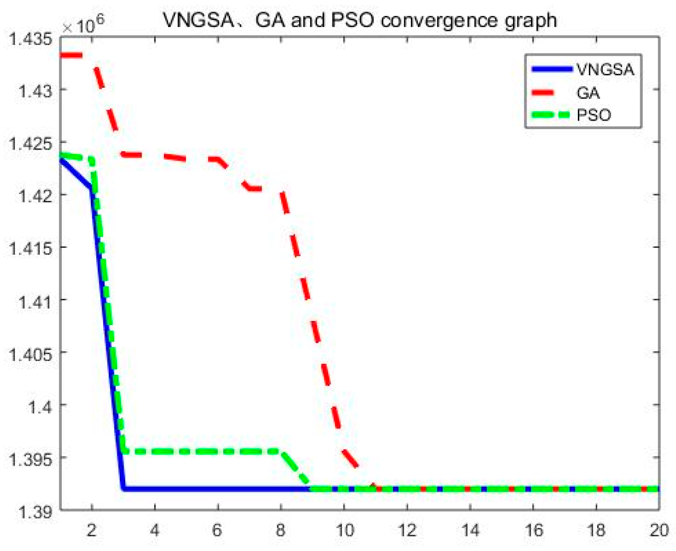
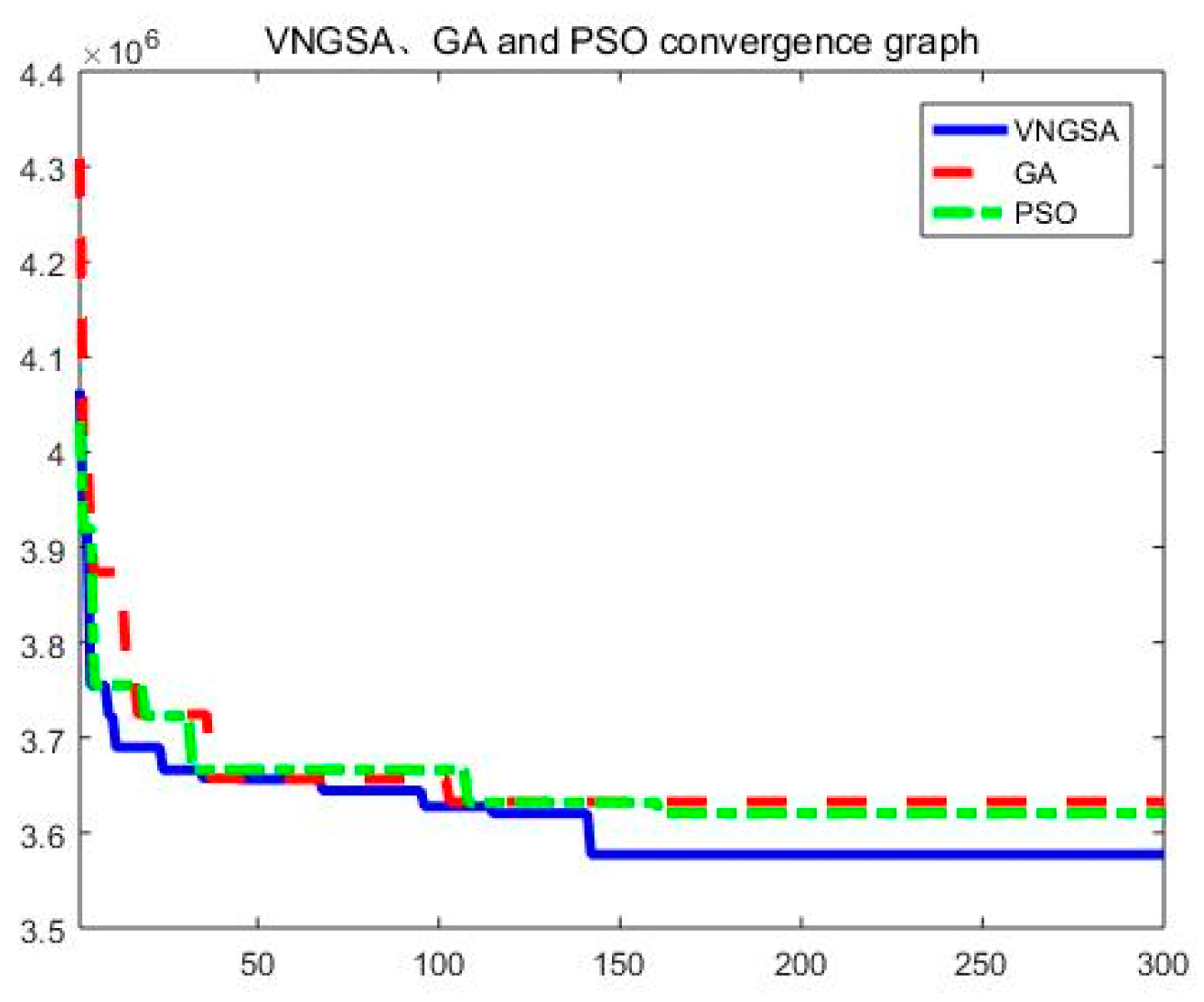
5.2. Computational Performance

To evaluate the efficiency of the variable neighborhood genetic simulated annealing algorithm in this paper, benchmark suites for tramp ship routing and scheduling problems are tested. Instances are from http://iot.ntnu.no/users/larsmahv/benchmarks/. This standard example, which solves multiple tramp ship scheduling problems with hard time windows, sums up the costs from operating the fleet plus the costs of spot charters. Constraints include port time window, ship capacity, etc. Standard examples are different from this paper is lacking speed constraints and carbon emissions costs. The computational tests were performed on MATLAB 2016a with Intel(R) Core (TM), 3.6 GHz processor and 8 GB of RAM under Windows 10.

The algorithm parameters depend on the size of the problem. The population size is 20–1000, and the number of generations is 15–1000. There are 15 groups of small, medium, and large instances, each considering a different combination of ships, time window nodes, and cargo. Each instance is labeled by using the values of the parameters. Hence, C8 indicates that the number of cargoes is eight, ships need to visit 16 ports, and V3 refers to 3 vessels. With each set of examples in the fleet of ship performance, the initial location of ports is different, as is indicated in

Table 3. The results comparison of standard examples.

Instance	Best	GA		PSO		VNGSA
		Z	%GAP	Z	%GAP	Z	%GAP
C8_V3_1	1,391,997	1,391,997	0.00	1,391,997	0.00	1,391,997	0.00
C8_V3_2	1,246,273	1,246,273	0.00	1,246,273	0.00	1,246,273	0.00
C8_V3_3	1,698,102	1,698,102	0.00	1,698,102	0.00	1,698,102	0.00
C8_V3_4	1,777,637	1,777,637	0.00	1,777,637	0.00	1,777,637	0.00
C8_V3_5	1,636,788	1,636,788	0.00	1,636,788	0.00	1,636,788	0.00
C16_V6_1	3,577,005	3,642,887	1.84	3,620,263	1.20	3,577,005	0.00
C16_V6_2	3,560,203	3,560,203	0.00	3,614,705	1.53	3,560,203	0.00
C16_V6_3	4,081,013	4,081,013	0.00	4,081,013	0.00	4,081,013	0.00
C16_V6_4	3,667,080	3,718,542	1.40	3,667,080	0.00	3,667,080	0.00
C16_V6_5	3,438,493	3,476,347	1.10	3,468,662	0.88	3,438,493	0.00
C35_V13_1	2,986,667	3,531,066	18.23	3,408,526	14.12	3,252,532	8.90
C35_V13_2	3,002,974	3,147,092	4.80	3,139,321	4.54	3,002,974	0.00
C35_V13_3	3,084,339	3,226,146	4.60	3,350,027	8.61	3,149,614	2.12
C35_V13_4	3,952,461	4,202,921	6.34	4,191,942	6.06	4,093,356	3.56
C35_V13_5	3,293,086	3,507,983	6.53	3,495,537	6.15	3,370,315	2.35
AVE	-	-	2.99	-	2.87	-	1.13

. Results about standard numerical examples are produced by the proposed algorithm, particle swarm optimization algorithm (PSO) and the traditional genetic algorithm (GA), under the same iteration number and population size, each algorithm calculates the same example for 5 times and takes the optimal value, where best is the known optimal solution, and Z obtains the optimal solution by the algorithm to calculate the gap values $\%GAP$:$\%GAP=\frac{Z-best}{best}\cdot 100\%$, where Z corresponds to the value obtained by the corresponding heuristic. AVE indicates the average values about the gap in this work.

Table 3 shows results for instances of 8, 16 and 32 cargoes corresponding to the small, medium and large size instances. In terms of the quality of solutions, using our VNGSA algorithm instead of the GA, the gap is considerably reduced from 2.99% to 1.13% on average. VNGSA algorithm instead of the PSO, the gap is considerably reduced from 2.87% to 1.13 % on average. We can see that the quality of optimal solutions by the VNGSA algorithm is better than the GA and the PSO. Additionally, the GA cannot find 7 optimum solutions and the PSO cannot find 8 optimum solutions, 11 optimal objective values are reached by the VNGSA algorithm. This VNGSA algorithm finds solutions even when the GA and the PSO are not able to find an optimum one. The Variable neighborhood genetic simulated annealing algorithm in this paper shows that this algorithm optimization ability is stronger and has superior solution performance. Figure 5 and Figure 6 show the convergence graphs for C8_V3_1 instance and C16_V6_1 instance. The graph shows the convergence of all three algorithms for two different problem instances. From the figures, it is amply clear that the VNGSA algorithm can converge quickly, the GA and the PSO trapped in local optima as it converges early for instance C16_V6_1.

5.3. Calculation of Examples

The computational performance proves the effectiveness of the proposed algorithm. Therefore, this algorithm is used to solve the tramp ship routing and scheduling with speed optimization considering carbon emissions. As pointed out in [22], ${\epsilon }_1=3.33$ and ${\epsilon }_2=3.11$. The calculation results are shown in

Table 4. Tramp ship routing and scheduling with speed optimization considering carbon emissions.

Ship ID	Route	Speed (knot)	Fuel Cost (K$)	Port Cost (K$)	Charter Cost (K$)	CO2 Emissions Cost (K$)	Total Cost (K$)
1	16-1-20	[12.6,14.4] [14.6,11.8] [12.7,11.2]	1583.7	1520.3	1160.0	93.5	4357.5
2	23-12	[13.7,13.2] [14.8,12.5]
3	19-27-29	[13.9,12.2] [11.2,11.2] [11.1,11.5]
4	4-25-11-10	[13.8,14.4] [13.7,14.3] [12.5,13.4] [14.1,13.2]
5	17-30-9-22-8	[11.6,14.4] [13.7,11.5] [15.0,11.6] [14.5,13.3] [13.0,13.5]
6	6-5-7-28-14-2	[12.2,12.0] [14.7,13.2] [11.6,12.0] [12.1,13.0] [15.3,13.9] [13.8,12.2]
7	21-13-3-26	[12.8,11.0] [11.8,11.4] [11.8,14.3] [12.5,11.6]
C	15-18-24	-

.

As we can see in Table 4, the owner ship is not idle, only 27 of the 30 cargoes are transported by owner ships, and the remaining cargo needs to be chartered. Due to the speed adjustment, the cost of CO₂ is $93,500, and the total cost is $4,357,500.

5.3.1. Multiple Optimal Speeds versus a Single Optimal Speed

In order to test the impact of different speed strategies on the economic benefits of shipping companies in the process of ship routing and scheduling, in this paper, we analyze the maximum speed, service speed, and variable speed strategy of the ship. The average speed of each ship is 14.97 knot for service speed.

Table 5. Speed strategy analysis.

Strategy	Ship ID	Route	CO2 Emissions (ton)	Fuel Cost (K$)	Port Cost (K$)	Charter Cost (K$)	CO2 Emissions Cost (K$)	Total Cost (K$)
Service speed	1	4-25-30-3-10	2174.58	2103.7	1626.3	998.1	122.2	4850.3
	2	27-13-26	2331.76
	3	17-7-14	2049.88
	4	23-11	504.39
	5	6-18-28-20	1723.42
	6	19-5-24-12-9-22-8	2004.99
	7	15-16-1-29-2	1434.02
	C	21	-
Max speed	1	1-14	2289.95	2307.8	1670.5	998.1	133.4	5109.8
	2	16-23-30-9-22	2651.80
	3	17-27	1119.41
	4	4-25-11-3-10	2149.59
	5	19-24-13-26	1691.03
	6	6-5-12-29- 2-8	1880.94
	7	15-18-7-28-20	1554.41
	C	21	-
Variable speed	1	16-1-20	1613.03	1583.7	1520.3	1160.0	93.5	4357.5
	2	23-12	707.38
	3	19-27-29	1419.38
	4	4-25-11-10	1770.17
	5	17-30-9-22-8	1545.02
	6	6-5-7-28-14-2	1030.56
	7	21-13-3-26	1265.76
	C	15-18-24	-

compares the various costs of the three speed strategies. C represents the charter ship.

From Table 5, we can see that if shipping enterprises always adopt the maximum speed, although they can transport more cargo by their owner ships and reduce charter cost, among all the costs, including fuel costs, port costs, and carbon emissions costs are the highest among the three strategies. Compared with the variable speed strategy, fuel cost is $724,100 higher and hence the cost of carbon emissions $39,900 higher. Therefore, the maximum speed strategy is the highest cost among all speed strategies. If the shipping enterprises adopt a fixed service speed, the number of cargoes that can be transported by owner ships is the same as the maximum speed, but due to the single speed, the fuel costs and port costs are higher than the corresponding costs under variable speed. Finally, the total cost is 10.2% higher than the total cost of variable speed. Therefore, it is a better choice for shipping enterprises to adopt variable speed in the process of transportation, which can reduce costs and carbon emissions, achieve profits, and have a positive effect on the environment. At the same time, we can see in the fourth column of Table 5 that in terms of the CO₂ emissions of each ship, because of different ship types and parameters, the ships transport more cargo, but their carbon emissions are less. Therefore, greener ships should be chosen as much as possible in the allocation of ships.

5.3.2. Results under Different Objective Functions

As mentioned, earlier in the discussion of models, by approaching the objective differently, we obtain different variations of the problem. Here we take numerical example 5.1 to examine the solutions of the following five variations: the alternative objective functions to be optimized are minimum fuel cost, minimum port cost, minimum charter cost, minimum CO₂ emissions cost, and minimum total cost.

Solutions can be found in

Table 6. Results under different objective functions.

Objective	Fuel Cost (K$)	Port Cost (K$)	Charter Cost (K$)	CO2 Emissions Cost (K$)	Total Cost (K$)
Min fuel cost	849.90	1136.4	7835.2	63.5	9885
Min port cost	1055.5	1087.8	8114.0	73.7	10,331
Min charter cost	2329. 5	1640.0	664.8	108.9	4743.2
Min CO2 emissions cost	852.1	1124.2	7835.2	63.2	9874.7
Min total cost	1583.7	1520.3	1160.0	93.5	4357.5

. It is important to know that different objective functions will generally produce very different solutions to the same problem. The objective is to minimize fuel costs, which results in an increased number of charter ships. In case the shipping company wants to minimize total CO₂ emissions, the result is similar to the minimize fuel cost objective. The reason is that the cost of carbon dioxide emissions mainly comes from fuel consumption in sailing. As can be seen from Table 6, the pursuit of minimum port cost is not beneficial to a shipping company. In practice, it is straightforward to see that with all objective functions, the best choices should help minimize total costs.

5.4. Sensitivity Analysis

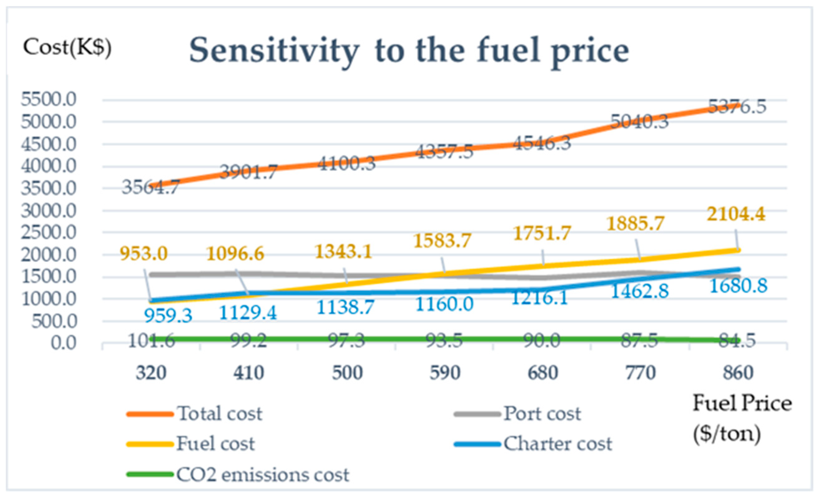
Since heavy fuel price is an important factor affecting the total cost, to investigate how fuel price and carbon emissions tax strategies affect the solution, we have tested instance 5.1 with different inputs of these parameters.

5.4.1. Fuel Price

To investigate how the fuel pricing affects the solution, we have tested instance 5.1 with different inputs of parameters, which provides the results when the heavy fuel price varies from $320 per ton to $860 per ton.

Figure 7 summarizes the results graphically, it is obvious that fuel prices are a very critical determinant of fuel costs, with the rise of fuel prices, the fuel cost is accordingly increased, and the charter cost is also increased. The reason is that high fuel costs make it impossible for some cargo to obtain profit by their owner ships. Therefore, charter ships are adopted. Since fuel cost is the main cost for shipping companies, the total cost increases with the rising fuel price.

To establish the linkage of fuel pricing with speed and carbon emission. We calculated total distance, total trip time, fuel consumption and average speed under different scenarios.

Table 7. The linkage of fuel pricing with speed and carbon emission.

Fuel Price ($/ton)	320	410	500	590	680	770	860
Total cost (K$)	3564.7	3901.7	4100.3	4357.5	4546.3	5040.3	5376.5
Port cost (K$)	1550.8	1576.5	1521.2	1520.3	1488.5	1604.3	1506.8
Fuel cost (K$)	953.0	1096.6	1343.1	1583.7	1751.7	1885.7	2104.4
Charter cost (K$)	959.3	1129.4	1138.7	1160.0	1216.1	1462.8	1680.8
CO2 emissions cost (K$)	101.6	99.2	97.3	93.5	90.0	87.5	84.5
Total distance (nautical miles)	77,219.4	72,145.0	73,134.6	74,174.4	73,335.2	70,977.3	69,455.5
Total trip time (days)	224.5	227.5	232.1	239.4	244.2	247.1	251.9
Fuel consumption (tons)	3249.2	3155.7	3100.6	2985.5	2873.2	2787.9	2699.6
Average speed (knot)	14.3	13.2	13.1	12.9	12.5	12.0	11.5
Used ships	7	7	7	7	7	7	7

summarizes the results about the linkage of fuel pricing with speed and carbon emission, where the results for CO₂ emissions cost, total trip time, fuel consumption and average speed are reflected. As can be seen from the results in all cases all ships are being used. In addition, when the fuel price increases, the ships would try to reduce the fuel consumption by taking shorter routes and sailing at a lower speed revealed from the increasing trip time. The reduction of speed affects CO₂ emissions cost. Finally, the table shows that increases in the fuel price lead to lower average speeds in order to reduce fuel costs and fuel consumption. Thus, slow speed will reduce carbon emissions and fuel consumption, increasing total trip time.

5.4.2. Carbon Emissions Taxation Strategy

In this section, we consider the effects of three cases on the solution. The first case is without carbon emissions cost, the second case considers carbon emissions costs based on emissions exceeding a certain threshold, and the third case considers tax costs based on carbon emissions. Computation results for three different calculations of carbon emissions costs are shown in

Table 8. Computation results for three different calculations of carbon emissions cost.

Strategy	Without Carbon Emissions Cost	Carbon Emissions Cost Based on Emission Exceed a Certain Threshold	Carbon Emissions Cost Based on Carbon Emissions
Fuel cost (K$)	2103.7	2066.2	2103.7
Port cost (K$)	1626.3	1630.0	1626.3
Chartering Cost (K$)	998.1	998.1	998.1
Carbon Emissions (K$)	-	93.7	122.2
Total cost (K$)	4728.1	4788.0	4850.3

.

It can be shown from Table 8 that both carbon emissions costs that exceed a certain threshold and carbon emissions costs based on carbon emissions will increase ship owner’s costs. However, we need to pay attention to environmental problems. Therefore, comparing two cases, carbon emissions costs that exceed a certain threshold are better than carbon emissions costs based on carbon emissions. It can reduce carbon emissions costs by $28,500. In the future, governments should be cautious in determining the suitable calculation method of carbon emissions costs.

6. Conclusions

Aiming at the joint tramp ship routing and scheduling and speed optimization, this paper considers the impacts of carbon emissions, the configuration of owner ships and charter ships, and speed on ship routing and scheduling. This paper established a model of tramp ship routing and scheduling with speed optimization considering carbon emissions with the objective of minimizing the total cost of shipping companies. A Variable Neighborhood Genetic Simulated Annealing (VNGSA) algorithm is used to solve the problem, and the applicability of the proposed models and the efficiency of the algorithm is verified by an example. The results show that: (a) Joint optimization of ship scheduling and speed can reduce fuel costs and carbon emissions costs. (b) Different objective functions will generally produce very different solutions to the same data, and greener ships should be used more. (c) The proposed algorithm matches ship type with cargo, and then according to the time constraints, the solution quality can be improved by using the neighborhood search strategy. (d) When the costs of chartering a ship are much higher than fuel costs, the shipping company can increase the number of cargoes transported by owner ships and reduce the number of chartered ships in the spot market. When the fuel price is too high, the number of chartered ships can be increased, reducing the cost of fuel, which is generated by transporting cargo by their owner ships. With the increase in fuel price, lower average speeds will be taken in order to reduce fuel costs and fuel consumption.

The research results not only deepen the theoretical research of tramp ship scheduling but also provide theoretical guidance and a decision basis for solving the joint optimization problem of ship scheduling and speed. Future research can focus on real-time ship scheduling in a dynamic environment. Based on the contributions presented in this paper, the next stage of the research will be focused on a dynamic environment and the increased allocation of ships and cargo.

References

1. International Maritime Organization. Third IMO Greenhouse Gas Study 2014; IMO: London, UK, 2014. [Google Scholar]
2. Buhaug, Ø.; Corbett, J.J.; Endresen, Ø.; Eyring, V.; Faber, J.; Hanayama, S.; Lee, D.S.; Lee, D.; Lindstad, H.; Markowska, A.Z.; et al. Second IMO GHG Study; International Maritime Organization (IMO): London, UK, 2009. [Google Scholar]
3. Thai, V.V.; Tay, W.J.; Tan, R.; Lai, A. Defining Service Quality in Tramp Shipping: Conceptual Model and Empirical Evidence. AJSL 2014, 30, 1–9. [Google Scholar] [CrossRef]
4. De Armas, J.; Lalla-Ruiz, E.; Expósito-Izquierdo, C.; Landa-Silva, D.; Melián-Batista, B. A hybrid GRASP-VNS for ship routing and scheduling problem with discretized time windows. Eng. Appl. Artif. Intell. 2015, 45, 350–360. [Google Scholar] [CrossRef]
5. Hennig, F.; Nygreen, B.; Furman, K.C.; Song, J. Alternative approaches to the crude oil tanker routing and scheduling problem with split pickup and split delivery. Eur. J. Oper. Res. 2015, 243, 41–51. [Google Scholar] [CrossRef]
6. Lee, J.; Kim, B.I. Industrial ship routing problem with split delivery and two types of vessels. Exp. Syst. Appl. 2015, 42, 9012–9023. [Google Scholar] [CrossRef]
7. Hemmati, A.; Hvattum, L.M.; Fagerholt, K.; Norstad, I. Benchmark Suite for Industrial and Tramp Ship Routing and Scheduling Problems. INFOR 2014, 52, 28–38. [Google Scholar] [CrossRef]
8. Hemmati, A.; Stalhane, M.; Hvattum, L.M.; Andersson, H. An effective heuristic for solving a combined cargo and inventory routing problem in tramp shipping. Comput. Oper. Res. 2015, 64, 274–282. [Google Scholar] [CrossRef]
9. Siddiqui, A.W.; Verma, M. A bi-objective approach to routing and scheduling maritime transportation of crude oil. Transp. Res. Part D Transp. Environ. 2015, 37, 65–78. [Google Scholar] [CrossRef]
10. Wu, L.X.; Pan, K.; Wang, S.; Yang, D. Bulk ship scheduling in industrial shipping with stochastic backhaul canvassing demand. Transp. Res. Part B. 2018, 117, 117–136. [Google Scholar] [CrossRef]
11. Norstad, I.; Fagerholt, K.; Laporte, G. Tramp ship routing and scheduling with speed optimization. Transp. Res. Part C Emerg. Technol. 2011, 19, 853–865. [Google Scholar] [CrossRef]
12. Hvattum, L.M.; Norstad, I.; Fagerholt, K.; Laporte, G. Analysis of an exact algorithm for the vessel speed optimization problem. Networks 2013, 62, 132–135. [Google Scholar] [CrossRef]
13. Meng, Q.; Wang, S.A.; Chung, Y.L. A tailored branch-and-price approach for a joint tramp ship routing and bunkering problem. Transp. Res. Part B Methodol. 2015, 72, 1–19. [Google Scholar] [CrossRef]
14. De, A.; Wang, J.; Tiwari, M.K. Fuel Bunker Management Strategies Within Sustainable Container Shipping Operation Considering Disruption and Recovery Policies. IEEE Trans. Eng. Manag. 2019, 1–23. [Google Scholar] [CrossRef]
15. De, A.; Wang, J.; Tiwari, M.K. Hybridizing basic variable neighborhood search with particle swarm optimization for solving sustainable ship routing and bunker management problem. IEEE Trans. Intell. Transp. Syst. 2019, 1–12. [Google Scholar] [CrossRef]
16. Li, X.J.; Xie, X.L. Integrated optimization of cargo distribution and ship speed for Heavy-Cargo transportation. J. Southwest Jiao Tong Univ. 2015, 50, 747–754. [Google Scholar]
17. Li, Z.; Pan, X.M. Research on optimization algorithm of ship speed. Ship Sci. Technol. 2016, 38, 7–9. [Google Scholar]
18. Wen, M.; Ropke, S.; Petersen, H.L.; Larsen, R.; Madsen, O.B.G. Full-shipload tramp ship routing and scheduling with variable speeds. Comput. Oper. Res. 2016, 70, 1–8. [Google Scholar] [CrossRef]
19. Yu, C.; Wang, Z.H.; Gao, P. Speed optimization considering dispatch and demurrage of the tramp shipping. J. Transp. Syst. Eng. Inform. Technol. 2018, 18, 195–201. [Google Scholar]
20. Psaraftis, H.N.; Kontovas, C.A. Speed models for energy-efficient maritime transportation: A taxonomy and survey. Transp. Res. Part C Emerg. Technol. 2013, 26, 331–351. [Google Scholar] [CrossRef]
21. Psaraftis, H.N.; Kontovas, C.A. Ship speed optimization: Concepts, models and combined speed-routing scenarios. Transp. Res. Part C Emerg. Technol. 2014, 44, 52–69. [Google Scholar] [CrossRef]
22. Wang, C.; Xu, C. Sailing speed optimization in voyage chartering ship considering different carbon emissions taxation. Comput. Ind. Eng. 2015, 89, 108–115. [Google Scholar] [CrossRef]
23. Wen, M.; Pacino, D.; Kontovas, C.A.; Psaraftis, H.N. A multiple ship routing and speed optimization problem under time, cost and environmental objectives. Transp. Res. Part D Transp. Environ. 2017, 52, 303–321. [Google Scholar] [CrossRef]
24. Yigit, K.; Acarkan, B. A new electrical energy management approach for ships using mixed energy sources to ensure sustainable port cities. Sustain. Cities Soc. 2018, 40, 126–135. [Google Scholar] [CrossRef]
25. Dere, C.; Deniz, C. Load optimization of central cooling system pumps of a container ship for the slow steaming conditions to enhance the energy efficiency. J. Clean. Product. 2019, 222, 206–217. [Google Scholar] [CrossRef]
26. De, A.; Mamanduru, V.K.R.; Gunasekaran, A.; Subramanian, N.; Tiwari, M.K. Composite particle algorithm for sustainable integrated dynamic ship routing and scheduling optimization. Comput. Ind. Eng. 2016, 96, 201–215. [Google Scholar] [CrossRef]
27. De, A.; Kumar, S.K.; Gunasekaran, A.; Tiwari, M.K. Sustainable maritime inventory routing problem with time window constraints. Eng. Appl. Artif. Intell. 2017, 61, 77–95. [Google Scholar] [CrossRef]
28. De, A.; Choudhary, A.; Tiwari, M.K. Multiobjective Approach for Sustainable Ship Routing and Scheduling With Draft Restrictions. IEEE Trans. Eng. Manag. 2017, 99, 1–17. [Google Scholar] [CrossRef] [Green Version]
Figure 1. Ship routing and scheduling with a single speed.
Sustainability 11 06367 g001
Figure 2. Ship routing and scheduling with variable speeds.
Sustainability 11 06367 g002
Figure 3. Process flowchart of proposed algorithm.
Sustainability 11 06367 g003
Figure 4. Variable neighborhood search strategy.
Sustainability 11 06367 g004
Figure 5. Convergence graph for instance C8_V3_1.
Sustainability 11 06367 g005
Figure 6. Convergence graph for instance C16_V6_1.
Sustainability 11 06367 g006
Figure 7. Sensitivity to the fuel price.
Sustainability 11 06367 g007