Application of a Adaptive Neuro-Fuzzy Technique for Projection of the Greenhouse Gas Emissions from Road Transportation

Abstract

In the past, different forecasting models have been proposed to predict greenhouse gas (GHG) emissions. However, most of these models are unable to handle non-linear data. One of the most widely known techniques, the Adaptive Neuro-fuzzy inference system (ANFIS), can deal with nonlinear data. Its ability to predict GHG emissions from road transportation is still unexplored. This study aims to fulfil that gap by adapting the ANFIS model to predict GHG emissions from road transportation by using the ratio between vehicle-kilometers and number of transportation vehicles for six transportation modes (passenger cars, motorcycle, light trucks, single-unit trucks, tractors, and buses) from the North American Transportation Statistics (NATS) online database over a period of 22 years. The results show that ANFIS is a suitable method to forecast GHG emissions from the road transportation sector.

1. Introduction

One of the most significant environmental issues in the world remains to be air pollution. This has resulted from the high levels of greenhouse gases (GHGs) in the atmosphere [1]. Moreover, one of the greatest contributors to global GHG emissions is the transportation sector. The increasing number of vehicles worldwide has led to a tremendous rise in GHG emissions. In 2007, 23% of the total worldwide GHG emissions came from the transportation sector. The estimate indicated that 73% of this was from the road transport sector [2].

In the recent past, there has been huge concern about the growing effects and implications of GHG emissions on our surroundings. These concerns have led to the development of many initiatives that aim at reducing the GHG emissions across the whole world [3].

Several approaches have been put forward to carry out predictions of GHG emissions. However, the accuracy of these approaches has been hugely affected by the lack of incorporation of non-linear variables in the model. It has also been noted that the amount of emissions emanating from road traffic is highly uncertain [4]. Given the uncertainity and complex interaction of variables contributing to GHG emosssions, consideration of non-linear variables relationships is important when developing a forecasting tool for GHG emissions in order to improve the reliability of the model’s predictions.

It is usually very complex to model environmental data because of the underlying correlation between multiple variables resulting in complex network relationships. Therefore, many researchers are working towards improving the forecast for GHG emissions. As such, several approaches have been proposed in the literature to predict GHG emissions. Historical data have played an important role for development of those models. Based on the literature review, it has been established that the majority of the prediction methods aim at improving the accuracy of the results [1].

A number of researchers [5,6] have succeeded in applying the Adaptive Neuro-fuzzy inference system (ANFIS) to model and forecast CO₂ emissions in various fields. ANFIS is a type of adaptive network that incorporates both neural networks and fuzzy logic principles, and can handle both linear and nonlinear parameters. However, to the authors’ knowledge, the use of the ANFIS approach to predict GHG emissions from the road transportation sector is not available in the literature.

Objective and Scope of Study

This paper aims to adapt and test the ANFIS Method to predict GHG emissions from the road transportation sector. We used the ratio between vehicle kilometer traveled (VKT) and the number of transportation vehicles (NTV). The ratio considers the six modes of transport (passenger cars, motorcycle, light trucks, single-unit trucks, tractors, and buses) for model development. The model will calculate the GHG emissions generated from the road transportation sector. Therefore, it will be a valuable resource for planners to forecast GHG emissions from different modes of transport and develop appropriate measures to reduce GHG emissions from the road transportation sector.

The rest of the paper is organized as follows: the next section provides a literature review followed by the research methodology. Results obtained from the adaptive neuro-fuzzy technique to predict and forecast the greenhouse gas emissions are presented next. The last section presents the conclusions and recommendations for future research.

2. Literature Review

It has been revealed from the review of the literature that emission factors in the transport sector have been considered in several studies across many countries. These factors are heavily affected by transport routes, and the age and size of the vehicles used [7].

There have been lots of findings in existing literature from various scholars which are aimed at bolstering the understanding of GHG emissions, as well as depicting the strategies to reduce GHG emissions. Our review of literature on the GHG emissions from the transport sector reveals that the methods could be classified into five categories: a bottom-up approach, decomposition models, system optimization, time series, and regression analysis.

Van der Zwaan, Keppo [8] carried out an investigation on CO₂ emissions of transport divisions in Europe, and how they can be decarbonized. Additionally, other strategies that include the COPART III methodology have been used in the analysis of road transport emissions in Italy [9]. This method ws also applied to study emissions from vehicles in urban areas [10,11,12].

The CO₂ emissions has implications which alter modal shift, fuel mix, population, economic growth, transport energy intensity, and emission coefficients. Timilsina and Shrestha [13] conducted a decomposition analysis and found that the main variables for CO₂ emissions are the transportation energy intensity and economic growth. Furthermore, it has been established that economic growth plays an integral part when it comes to the contribution of CO₂ emissions in ASEAN-5 and EU27 economies [14,15]. After application of decomposition analysis, Lakshmanan and Han [16] determined that the population number and GDP were the main causes of CO₂ discharges in the transport sector. Alternatively, Li, [17] used Kaya identity and the Logarithmic Mean Division Index (LMDI) to decompose the CO₂ emissions of urban freight, identify the main determinants of emissions change, and to use those determinants to predict CO₂ emissions from the transport sector. Moreover, Fan and Lei [18] built a multivariate generalized Fisher index (GFI) decomposition model based on the expanded Kaya identity to measure the influence of the energy structure, energy intensity, output value of per unit traffic turnover, transportation intensity, economic growth and population size on carbon emissions in the transportation sector of Beijing.

The system optimization method has been widely used in the forecasting of CO₂ emissions and energy demand [19,20,21]. Additionally, it has been used in the process of planning networks that can help in energy supply activities [22]. It has also been used in analyzing strategies that can lead to better energy planning, which promotes sustainable development [23].

Several optimisation models have been proposed in the literature that estimate CO₂ emissions and recommend strategies to reduce CO₂ emissions. By utilizing linear programming models, several studies examined benefits associated with energy choices that could support the reduction of CO₂ by industries [24,25,26]. Moreover, a mixed-integer linear programming model has been proposed by researchers [27] that further sheds light on the effects of fuel switching and balancing on power generation. Reference [27] established that fuel efficiency (FE) switching was the best choice for decreasing discharges of CO₂. This was backed up by another study by Tan, Hashim [28] who used mixed-integer linear programming to achieve a perfect arrangement of waste to vitality in order to ensure reduction costs were related to CO₂ emissions and generation of electricity.

After utilization of time series analysis, Saboori et al. [27] explored the long run nexus between the emissions of CO₂ by the transport sector and economic growth in OECD nations. There has been a substantial focus on predicting the CO₂ emissions trends from the vehicles, vehicular energy intake and population in order to improve management of CO₂ emissions in Taiwan [29]. Meyer, Leimbach [30], provide an estimate of the demand of passenger cars in 11 world regions and the associated CO₂ emissions. Furthermore, panel data has been used by Tokunaga and Konan [31] and Konur [32], in order to provide estimations of CO₂ which are caused by the transportation sector. Moreover, Tolón-Becerra and Pérez-Martínez [33] focus on the targets set by EU countries towards the reduction of CO₂ emissions. Sultan [34] was able to find out that there existed a co-combination of fuel price (FP) and pay per capita on transport fuel consumption (FC). There was also a discovery of a relationship between CO₂ discharges and vitality utilization, as noted by reference [35,36,37,38,39]. Begum, Sohag [40], delved at the impact of GDP, FC and populace development on the emissions of CO₂. Ivy-Yap and Bekhet [41], put forward recommendations that could help reduce CO₂ emissions which included the use of low-carbon advancements. Additionally, Talbi [42] looked at the impact of energy consumption, economic growth, urbanization, and fuel rate on CO₂ emissions using the Vector Autoregressive (VAR) model and analyzed the influencing factors of the changes in CO₂ emissions from the transportion sector.

By using regression analysis, Sadorsky [43] looked into the relationship between GDP, salary, urbanization, and vitality force and found that diminishing CO₂ emissions could develop from an increase in fuel changing and fuel efficiency (EF) to renewable vitality. High population density which led to thick road networks in urban areas could create a better absorption of emitted CO₂ [44]. Alhindawi et al. [45] identified the main drivers of greenhouse gas emissions for the road sector by using the ratio between vehicle-kilometers and number of transportation vehicles for six transportation modes. Additionally, Xu, He [46] concluded that there were effects of vitality structure, populace, vitality intensity, and GDP on emanations of CO₂. GDP was found to be the main driving force behind major emanations of CO₂, followed by the scale of the populace and vitality structure. Furthermore, Friedrich and Trois [47] combined the regression analysis and the life cycle assessment approach to predict the GHG emissions for solid waste management, utilizing specific emission factors for different waste management processes and included upstream, downstream, and operational GHG emissions. The autoregressive distributed lag (ARDL) approach was used by Alshehry and Belloumi [48] to study the relationship between transport CO₂ emissions, road transport energy consumption, and economic activity in Saudi Arabia. Lin and Benjamin [49] looked at the impact of gross domestic product GDP per capita, energy intensity (EI), carbon intensity (CI), and total population on carbon dioxide emissions in China’s transport industry using quantile regression analysis, and the results showed that GDP, energy intensity, and carbon intensity have a greater impact on carbon emissions than urbanization. Meanwhile, Danish, Baloch [50] investigated the relationship between transport energy consumption, economic growth, and carbon dioxide emissions to account for Foreign direct investment (FDI) and urbanization by applying autoregressive distributive lag (ARDL) and vector error correction model (VECM). The results also indicated a strong significant impact of transport energy consumption on CO₂ emissions from the transportation sector. Several studies have successfully applied ANFIS for forecasting scenarios in different fields including automatic control and decision analysis [51,52], and all have shown a high accuracy rate [53,54]. Jang and Chuen-Tsai [55] listed the applications of the neuro-fuzzy approach while also describing the theoretical basis of the model.

This section reviewed the body of knowledge relative to the analysis of the tools and methods used for prediction of the GHG emissions along with their pros and cons.

Table 1. Comparision of Pros and Cons of different forecasting techniques.

Techniques	Pros	Cons
Bottom-up approach	▪ Able to determine a typical end-use energy consumption ▪ Encompasses occupant behaviors ▪ Does not require detailed data (only billing data and simple survey information) ▪ Easy to develop and use	▪ Relies on historical consumption data ▪ Limited capacity to assess the impact of retrofited or new technologies ▪ Provides fewer data and less flexibility ▪ Requires large survey sample ▪ Multicollinearity
Decomposition models	▪ It is easy to understand	▪ The cycle component must be input by the forecaster since it is not estimated by the algorithm.
System optimization	▪ Can be simple to implement ▪ Have few parameters to adjust ▪ Able to run parallel computation ▪ Can be robust	▪ Can be difficult to define initial design parameters ▪ Cannot work out the problems of scattering
Time series analysis	▪ It is a very effective method of forecasting because it makes use of the seasoned patterns. ▪ It helps to understand the past behavior and would be helpful for future predictions. ▪ It helps us to compare the present performance of the series with that of the past. ▪ It helps to compare the performance of two different series of a different type for the same time duration.	▪ It is costly because the forecasts are based on the historical data patterns that are used to predict the future market behavior. ▪ The conclusion drawn from the analysis of time series is not always perfect. ▪ The various factors that affected the fluctuations of a series cannot be fully adjusted by the time series analysis. ▪ The various factors that influence the time series may not remain the same for an extended period of time and so forecasting made on this basis may become unreliable.
Regression analysis	▪ Easy to implement and interpret	▪ It involves a very lengthy and complicated procedure of calculations and analysis.
Neuro-Fuzzy inference system (ANFIS)	▪ Ability to change the qualitative aspects of human knowledge into the process of precise quantitative analysis	▪ Time-consuming

and

Table 2. Summary of literature review outlining the key features, including methodolog.

Author/Year	Methodology/Approach
	COPERT III	Johansen Cointegration	Granger Causality	Linear Programming	Time Series	Autoregressive Distributed Lag (ARDL) Approach	Logarithmic Mean Division Index (LMDI)	Vector Error Correction Model VECM	System Optimization	Vector Autoregressive (VAR)model	Autoregressive Integrated Moving Average (ARIMA)	Seasonal Autoregressive Integrated Moving Average (S-ARIMA)	Toda–Yamamoto	Decomposition	Life Cycle Assessment (LCA)	Regression Analysis	Double Exponential Smoothing	ANFIS
Horikawa, Furuhashi, and Uchikawa (1992)																		x
Jang (1993)																x
Jang and Chuen-Tsai (1995)																		x
Bai and Wei (1996)				x
Lakshmanan and Han (1997)														x
Shi and Mizumoto (2000)																x
YEH, TSAY, and LIANG (2005)																		x
Hashim et al. (2005)				x
Ediger and Akar (2007)											x	x
Meyer, Leimbach, and Jaeger (2007)					x
Bellasio et al. (2007)	x
Ang (2008)		x
Wang et al. (2008)									x
Lu, Lewis, and Lin (2009)					x
Bekhet and Yusop (2009)		x
Timilsina and Shrestha (2009)														x
Khajeh, Modarress, and Rezaee (2009)													x					x
Zhou, Chan, and Tontiwachwuthikul (2010)																		x
Sultan (2010)					x	x
Borjesson and Ahlgren (2012)				x
Shu and Lam (2011)																x
Wang et al. (2011)														x
Andreoni and Galmarini (2012)														x
Tolón-Becerra et al. (2012)																x
Si et al. (2012)									x
Bekhet and Yasmin (2013)			x		x	x
Tan et al. (2013)				x
Chandran and Tang (2013)		x	x					x
He and Chen (2013)	x
Dallmann et al. (2013)	x
Kanzian et al. (2013)									x
Sider et al. (2013)	x
Sadorsky (2014)																x
Xu et al. (2014)														x
Ahanchian and Biona (2014)									x
Motasemi et al. (2014)									x
Szendrő and Török (2014)									x
Saboori, Sapri, and bin Baba (2014)					x
Tokunaga and Konan (2014)																x
Konur (2014)																x
Xu, He, and Long (2014)																x
Begum et al. (2015)					x	x
Ivy and Bekhet (2015)					x	x
Friedrich, E., & Trois, C. (2016)															x	x
Alhindawi et al. (2016)																x
Li et al. (2016)							x
Fan, F., & Lei, Y. (2016)														x
Alshehry et al. (2017)			x			x
Talbi, B. (2017)					x					x
Lin, B., & Benjamin, N. I. (2017)																x
Danish et al. (2018)						x		x

provide a summary of methodology adopted in the existing literature to predict GHG emissions in various industry sectors along with the associated pros and cons. where Table 1 and Table 2 are the authors own synthesis from the literature. As can be seen, the ANFIS method has been less examined, particularly fpr predicting GHG emissions from the road transportation sector.

3. Model Development

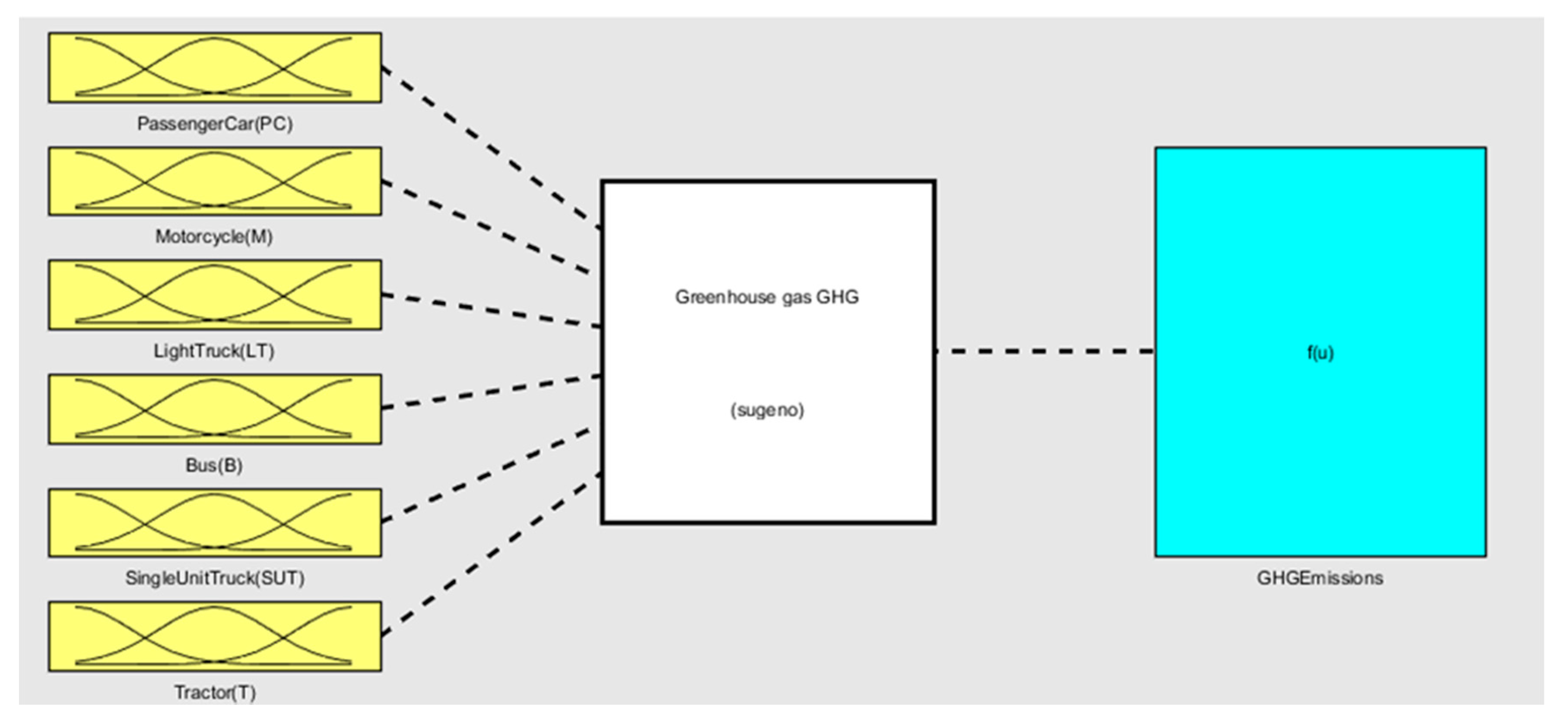
As observed from the literature review above, a variety of methods exist which are used in the computation of GHG emissions. However, there is a difference in their assumptions and scope, since they are reliant on data gathered from various countries. As a result of this disparity, there has been huge variations in the results obtained. Thus, this leads to the need for having a robust and flexible approach which can accommodate a substantial amount of data and a non-linear variables relationship by ensuring a reasonable accuracy of GHG emissions predictions. Therefore, the prime goal of this study is to provide a general approach which can be used in analyzing and recognising various factors that influence the GHG emissions from the road transportation sector. We adapted the neuro-fuzzy technique to achieve this objective.

ANFIS is functionally equivalent to a Sugeno-type fuzzy rule base [56] which makes use of a set of training data to adjust the base of the current rule to adapt to neuro-fuzzy. Training data are utilized to teach the neuro-fuzzy system by adjusting its variables and using a standard neural network algorithm, resulting in a reduced mean square output error [56].

3.1. Variables

3.1.1. Data Sources

We used historical data (1990–2012) of GHG emissions, the ratio between Vehicle-kilometres by Mode (VKM), and the Number of Transportation Vehicles (NTVs) for six different road vehicle modes (passenger cars, motorcycle, light trucks, single-unit trucks, tractors, and buses) in North America. The data were extracted from the official online database of North American Transportation Statistics (NATS) [57].

VKM is the total kilometers traveled by different road vehicles on the highway system during a given period of time. This is an important variable for transport planning and is used in estimating vehicle emissions, environmental quality, and assessing traffic impact [58] Likewise, NTV that characterizes traffic volume is an important parameter to examine how the road network is being used, level of congestion and the time spent in the network. This will have implications for estimating the GHG emissions from road traffic.

The collected data has been used to carry out the analysis and identification of the various factors which influence GHG emissions.

Table 3. Data set for the Model (Ratio (Vehicle-kilometers Traveled by Mode (Millions of vehicle-kilometers)/Number of Transportation Vehicles (Equipment)).

Year *	GHG Emissions	Ratio (Vehicle-Kilometres by Mode (Millions of Vehicle-kilometers)/Number of Transportation Vehicles/Equipment)
		Passenger cars	Motorcycles	Light trucks	Bus	Single-unit trucks	Tractor
1990	1,235,100	16,951.2	3611.02	19,154.65	14,697.27	18,615.41	88,845.13
1995	1,352,700	18,029.19	4045.73	19,340.74	15,072.14	20,087.7	109,567.97
1996	1,388,200	18,234.27	4123.62	19,007.95	15,201.91	19,580.98	109,556.01
1997	1,416,900	18,637.02	4240.05	19,496.62	15,785.29	20,337.56	112,012.62
1998	1,461,200	18,915.58	4265.81	19,589.92	15,760.13	19,088.13	103,424.3
1999	1,511,800	19,068.06	4101.93	19,242.62	16,920.13	19,633.12	105,025.63
2000	1,521,500	19,273.95	3876.61	18,783.83	16,371.25	19,145.87	103,640.19
2001	1,527,400	19,028.74	3161.7	18,019.17	15,179.82	20,427.1	102,001.97
2002	1,562,500	19,636.86	3071.85	18,287.93	14,481.08	21,607.19	98,071.69
2003	1,571,300	19,833.21	2869.81	18,163.64	14,054.47	21,394.12	118,171.31
2004	1,604,400	20,052	2824.23	17,998.3	13,762.55	20,489.92	113,972.05
2005	1,612,100	20,132.35	2701.72	17,573.58	13,919.78	19,753.29	111,076.55
2006	1,609,800	20,093.44	2903.45	17,574.81	13,281.68	19,445.7	105,453.36
2007	1,614,100	17,236.04	4823.72	24,091.42	27,996.16	23,788.94	112,486.14
2008	1,540,100	16,560.69	4319.92	24,552.89	28,287.41	24,632.22	114,434.35
2009	1,500,100	16,704.39	4221.33	24,521.05	27,443.22	23,142.86	103,211.24
2010	1,509,000	17,144.27	3711.09	24,895.69	26,239.55	21,684.42	110,940.84
2011	1,489,900	17,089.15	3575.54	23,499.82	33,315.12	21,314.6	107,497.11
2012	1,487,100	18,128.56	4053.84	19,121.97	31,059.15	20,623.94	106,475.9

* This varies depending on the data. Generally, the data includes 1990, 1995–2012.

shows the complete set of the data used in this study.

3.1.2. Data Limitations

The US Department of Transportation is in charge of the NTV data, which is collected and stored in the database. This data covers all categories of vehicles which include combination truck tractors, light trucks, and passenger cars. Data collected from the light trucks categories include data of vans, pick-up trucks as well as sporty utility vehicles. The category of tractors also included data of tractors while on the other hand taxis were included under the passenger’s car category. Furthermore, local motors were included under the bus category [57].

On the other side, VKT data included motorcycles, light trucks, and passenger cars. The Department of Transportation in the US gave an updated VKT data using a highway mode for a long period of time. It was noted that there was a change in the classification of vehicles where some vehicles had relocated from the passenger’s category and moved to the truck category at some point in time [57].

Hence, based on that observation, we need to understand that time-series data is prone to discontinuities which can result in errors when we are performing estimation using a regression model. However, the proposed method to be used in this study as well as the generated results create room for further testing once a new, good, and detailed dataset is obtained.

3.2. Adaptive Neuro-Fuzzy Model (ANFIS)

The MATLAB ANFIS algorithm was used to develop the model as it offers a process for the fuzzy modeling to study information about a data set, in order to count the membership function (MF) variables that allow the connected Fuzzy Inference System (FIS) to follow the provided data set (input-output) [59].

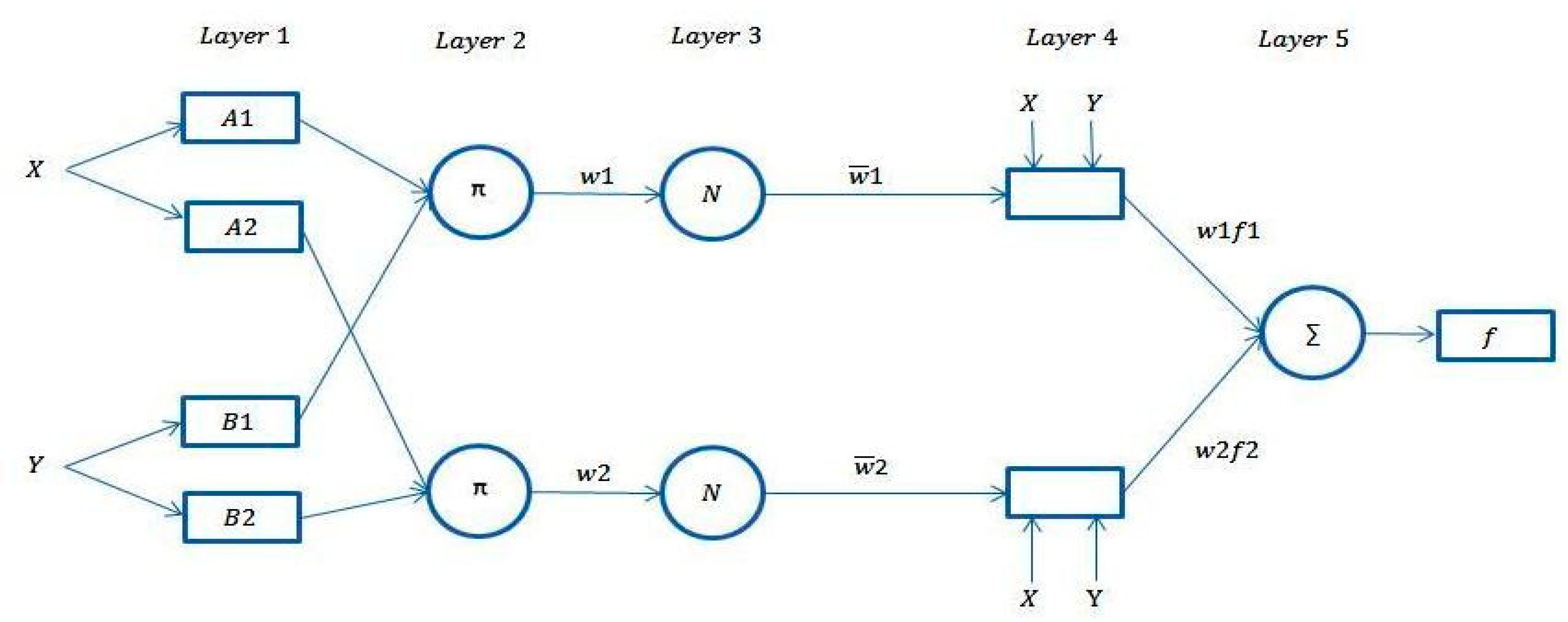
3.2.1. Learning Algorithm and Architecture of ANFIS

Figure 1 shows the ANFIS architecture. It is to be noted that for any input parameters, the output can be represented as a linear combination of the resulting parameters [50].

Each layer has different functions which is summarized as follows [60]:

Layer 1: The outputs are the membership values due to input samples and used membership functions. To clarify the structure. $x$ and $y$ are considered to be the input nodes, $A$ and $B$ are the linguistic labels, while ${\mu }_{Ai}$ and ${\mu }_{Bi}$ are the membership functions. Below are the outputs obtained from the nodes.

$$\begin{array}{c}{O}_i^1={\mu }_{Ai}\left(x\right)i=1,2\\ O_{i+2}^1={\mu }_{Bi}\left(x\right)i=3,4\end{array}$$

(1)

The membership functions ${\mu }_{Ai}$, and ${\mu }_{Bi}$ are generally presumed to be bell-shaped with the maximum and the minimum values of 1 and 0, respectively. Meanwhile $m_i$ is the middle point of the bell-shaped membership function and ${\sigma }_1$ is the standard deviation, $\mu \left(x\right)$ can be calculated as shown in Equation (2):

$$\mu \left(x\right)=\frac{1}{1+{\left\{\frac{x-c_i}{a_i}\right\}}^{2b_i}}$$

(2)

where $a_i$,$b_i,$ and $c_i$ are the premise parameters.

Layer 2: The firing strength in this layer of each rule is calculated as:

$$O_i^2=w_i={\mu }_{Ai}\left(x\right).{\mu }_{Bi}\left(y\right)fori=1,2$$

(3)

Layer 3: The normalization of the firing strengths is performed. The $i$th node calculates the ratio of the $i$th rules firing strength to all rules firing strength.

$$O_i^3=\overline{w_i}=\frac{w_i}{w_1+w_2}\mathrm{for}i=1,2$$

(4)

Layer 4: The output of each node is the product of the normalized firing strength and a first order polynomial. Where $f_1$ and $f_2$ are the fuzzy if-then rules, the outputs are written as given in the following equation:

• Rule 1: if $x$ is $A_1$ and $y$ is $B_1$ then $f_1$ = $p_{1}x+q_{1}y+r_1$
• Rule 2: if $x$ is $A_2$ and $y$ is $B_2$ then $f_2$ = $p_{2}x+q_{2}y+r_2$

$$O_i^4={\overline{w}}_i{f}_{\mathrm{i}}={\overline{w}}_i\left(p_{i}x+q_{i}y+r_i\right)$$

(5)

where linear $p$, $q,$ and $r$ are the consequent parameters.

Layer 5: The overall output of ANFIS in this layer will be computed as follows:

$$O_i^5={\displaystyle \sum _i}{\overline{w}}_i{f}_i=\frac{{\sum }_i{w}_i{f}_i}{{\sum }_i{w}_i}$$

(6)

The final output of ANFIS is expressed as:

$$f_{out}={\overline{w}}_1{f}_1+{\overline{w}}_2{f}_2=\frac{w_1}{w_1+w_2}{f}_1+\frac{w_2}{w_1+w_2}{f}_2=\left({\overline{w}}_{1}x\right)p_1+\left({\overline{w}}_{1}y\right)q_1+\left({\overline{w}}_1\right)r_1+\left({\overline{w}}_{2}x\right)p_2+\left({\overline{w}}_{2}y\right)q_2+\left({\overline{w}}_2\right)$$

(7)

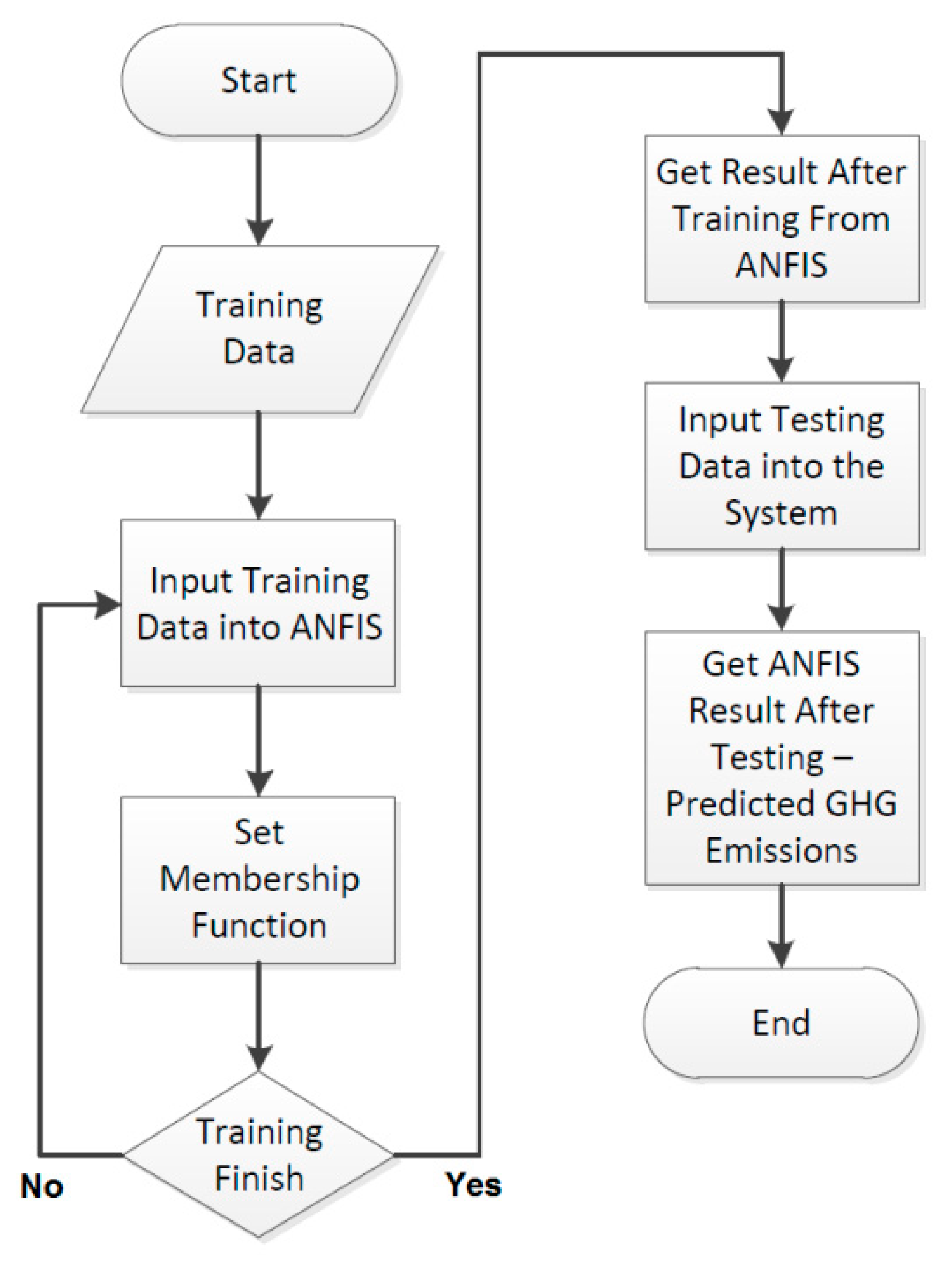
3.2.2. Division of the Data and developing the ANFIS Model

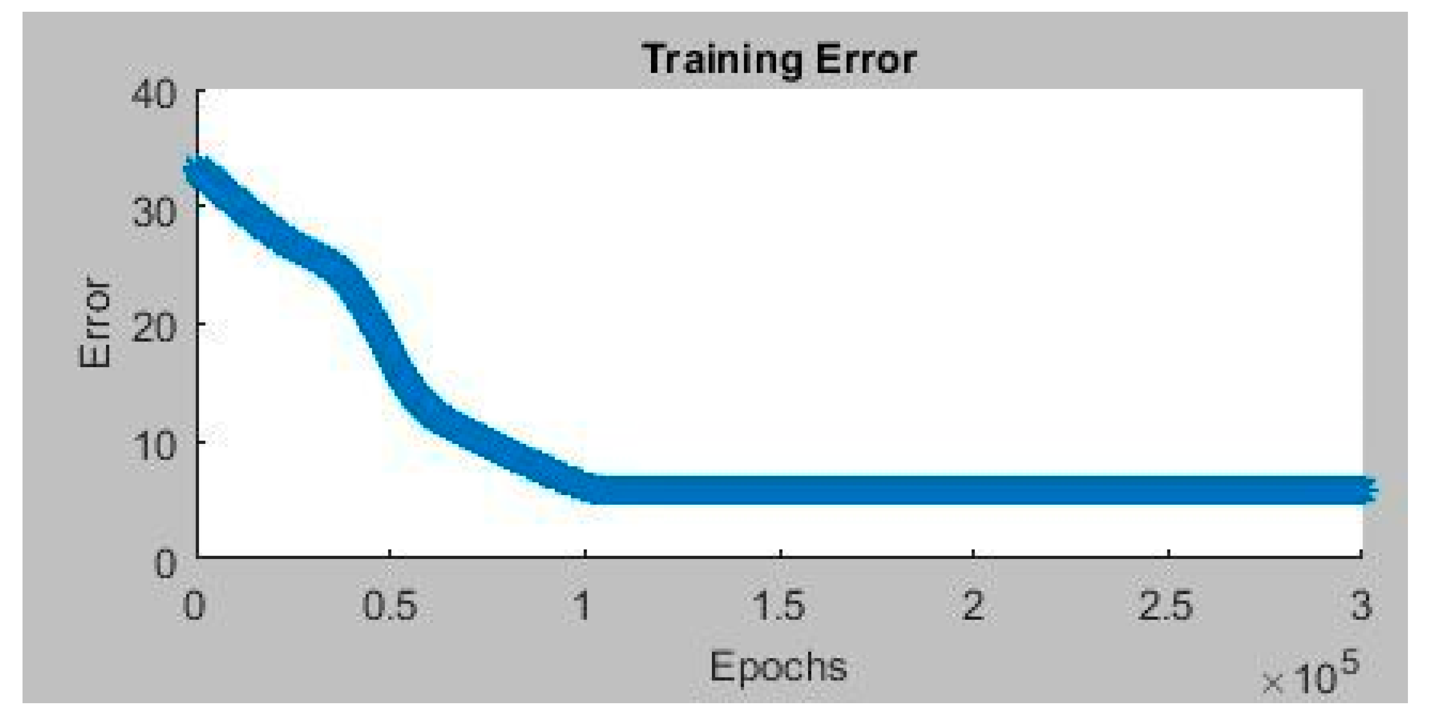
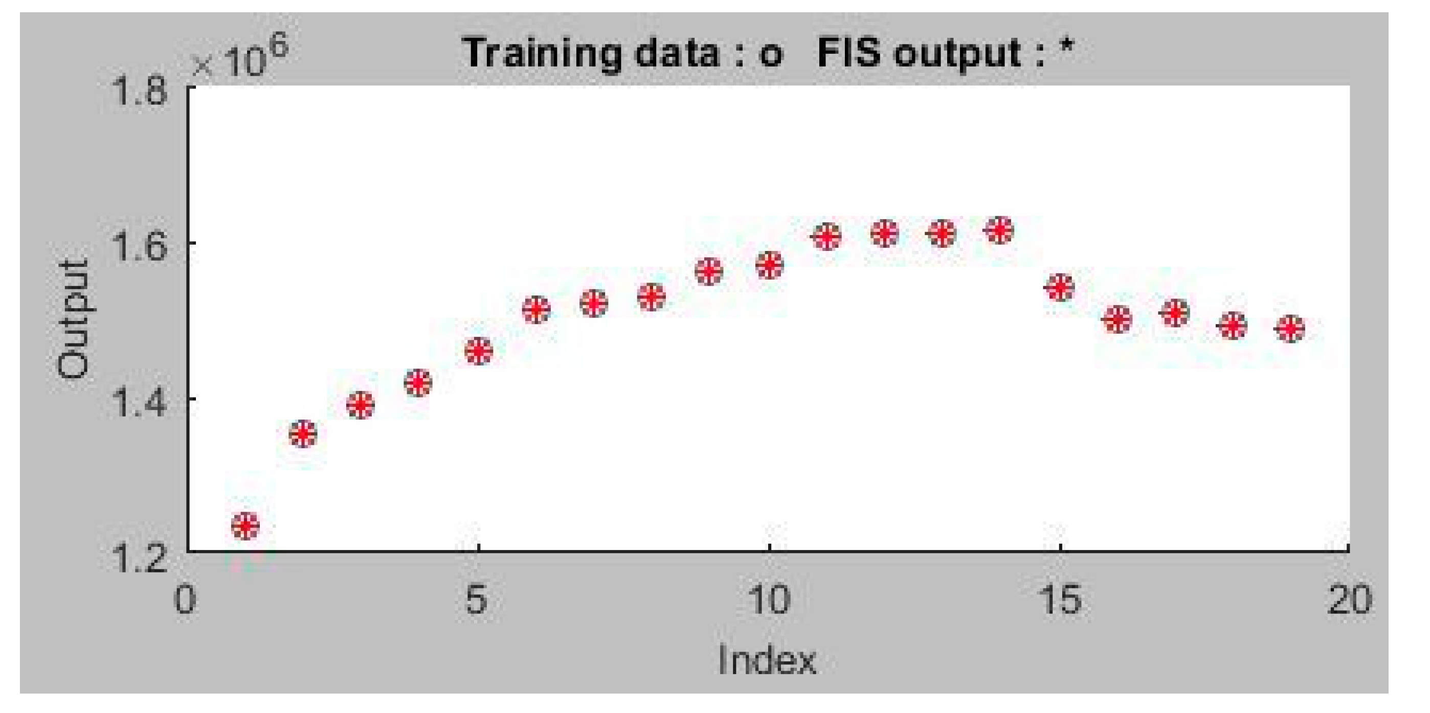
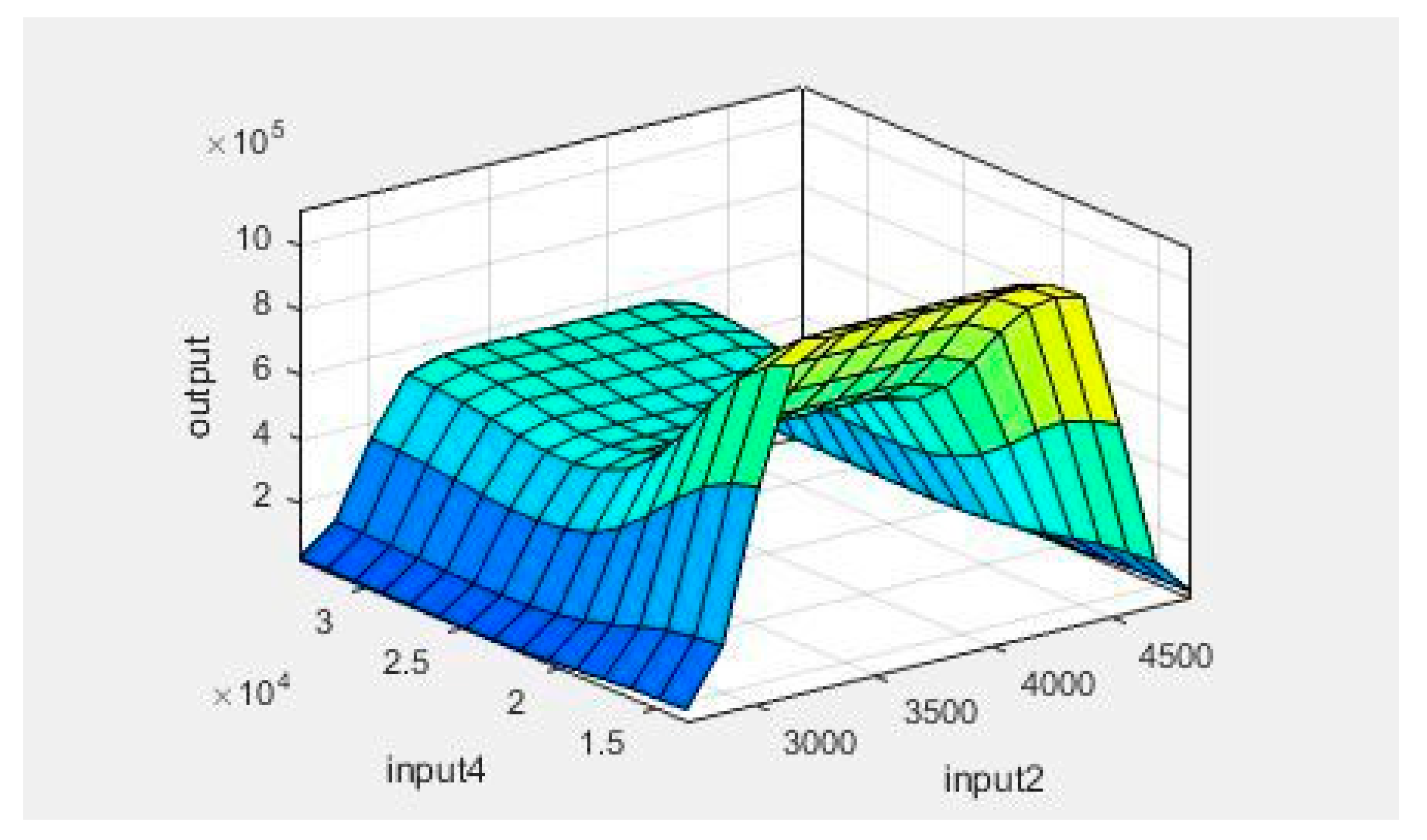
The NATS dataset was used to develop ANFIS modeling and the prediction of GHG emissions start by gaining a data set and dividing it into training and validating data. The training data is utilized to find the initial assumed parameters for the membership functions by a model with an actual system for validating purposes. Figure 2 shows the ANFIS training and modeling process.

The first step in the development of the FIS is defining the types and number of membership functions for the input and output variables for ANFIS [61].

4. Results

The fuzzy logic toolbox of MATLAB 7 was utilized for this task. A Gaussian function was used to optimize the parameters. In addition, a total number of 1503 nodes were utilized in the ANFIS system to develop the fuzzy systems for modeling and forecasting the greenhouse gas emissions for the road sector. Optimization was conducted on a total number of fuzzy rules with N number of inputs, which is determined as [5],

$$\text{Number of fuzzy rules}=M^N\times T$$

(8)

where N is the number of model inputs, M the number of fuzzy MFs (Membership Function) representing each input, and T is the number of fuzzy MF representing the model output [5]. For example, in this study, since the number of membership functions linked with the six input variables is three, the 6-dimensional input space can be divided into $3^6$ = 729 subspaces, which means the FIS for GHG emissions will contain 729 rules based on the algorithm of grid dividing.

FIS was created after completing the training process.

The structure of ANFIS for greenhouse gas emissions is shown in Figure 3 where the f(u) is the final output of ANFIS and the Sugeno is the fuzzy model.

The membership functions of the six inputs are in the form of a Gaussian function, and the number of membership functions of all inputs is three, as shown in Figure 3 (in yellow brackets). A three Gaussian-type MF for each input resulted in highly accurate modeling and minimum training and validation errors. This analysis shows that all the variables have the same effect on the model and there is no variable more important than the others. The final MFs were updated by the ANFIS model to achieve a good mapping of the input variables to the greenhouse gas emissions output. Figure 3 shows the final fuzzy inference system used to predict the greenhouse gas emissions.

729 Sugeno-type rules make up the rule base. Given this, there were 729 output values which were calculated using the 729 linear functions since there were 729 rules in the FIS for GHG emissions. Assuming the 6 coefficients for the 6 inputs were ${\alpha }_i$,${\beta }_i$,${\delta }_i$,${\gamma }_i$,${\rho }_i$,${\lambda }_i$, and the constant was ${\epsilon }_i$, the ith rule would be as follows:

If Passenger Cars ($PC$) is $A_l$, Motorcycles ($M$) is $B_l$, Light Trucks ($LT$) is $C_l$, Bus ($B$) is $D_l$, Single Unit Trucks ($SUT$) is $E_l$, and Tractors ($T$) is $F_l$, then

$$O_i={\mathsf{\alpha }}_i\times \left(PC\right)+{\mathsf{\beta }}_i\times \left(M\right)+{\mathsf{\delta }}_i\times \left(LT\right)+{\mathsf{\gamma }}_i\times \left(B\right)+{\mathsf{\rho }}_i\times \left(SUT\right)+{\mathsf{\lambda }}_i\times \left(T\right)+{\mathsf{\epsilon }}_i\left(i=1,2,\dots \right)$$

(9)

where $A_l,B_l,C_l,D_l,E_l,F_l$, arer the linguistic labels of membership and functions for each input variable and $Oi$ is the output in the ith rule.

There were 19 training data points and 300,000 learning epochs that were used to complete the neural network training for building a fuzzy model for predicting the greenhouse gas emissions. As shown in Figure 4, to evaluate the functionality of the model, a root mean square error (RMSE) analysis was used. The results show that with a total number of 300,000 iterations, the minimum value of the RMES (5.7743) was reached. A comparison between the actual and ANFIS-predicted greenhouse gas emissions values after training is shown in Figure 5, where the Index is the number of years and the output is the GHG emissions (actual and predicted values). It can be seen that the results of the presented model were in good agreement with the obtained data, which shows that the system is well-tested to model the actual GHG emissions. The ANFIS-predicted GHG emission is shown in Figure 6 as a surface plot (showing the relation between input 2 and 4 (Motorcycles and Buses, respectively) and output (GHG emissions) of fuzzy inference system of GHG emissions as a function of the ratio Vehicle-kilometres by Mode (VKM) and Number of Transportation Vehicle (NTV) for Motorcycles ($M$) and Buses ($B$).

5. Discussions and Conclusions

The economic and health impacts of air pollution have caused it to become a major concern in many countries. People have become more aware of this issue because of the available information on how it negatively affects human health and environmental sustainability [1].

In the majority of the developed nations such as the OECD countries, GHG emissions from the road transport industry constitute a large proportion of total GHG emissions from the transportation sector at large. In order to cut these emissions, coordinated efforts should be made to reduce emissions from the transport industry.

To date, models that forecast GHG emissions have a lot of constraints, particularly due to the unavailability of detailed data (e.g., fuel consumption per vehicle, average annual distance traveled). The use of numerous equations has also been reproached because of the need to satisfy many assumptions. In addition, the methodology and assumptions made are too rigid, which makes such equations difficult to be used in practice [58]. Recently, adaptive neuro-fuzzy inference systems (ANFIS) has been applied in different fields as a forecasting tool as it is more efficient and less time-consuming in modeling complex system compared to other mathematical models [62].

The proposed ANFIS method was applied to forecast GHG emissions from the road transportation sector in North America using over 20 years of data on GHG emissions, ratio of Vehicle-kilometers by Mode (VKM) and Number of Transportation Vehicle (NTV). The ratio considered the six modes of transport (passenger cars, motorcycle, light trucks, single-unit trucks, tractors, and buses).

The ANFIS analysis shows that all the variables (different modes of transport) have the same impact on the model, and there is no variable that is more important than the others. This attests to the reliability of the ANFIS model in optimizing the prediction of GHG emissions. In addition, this study shows how the ANFIS method can be utilized to model and predict GHG emissions from the road transportation sector. Here, we only used the data set from one country to test the model. In the future, similar data sets from other countries may be used (as they become available) to test the robustness of the method and average geographical bias. Furthermore, it is to be acknowledged that our forecasting was based on the results of historical data and may not include new technologies, processes, and systems that may be introduced in the future; hence, the model may need to be re-tested with newer sets of data which could further refine the model. Nevertheless, the generality of the approach should be applicable to forecast the GHG emissions.

Road vehicles are a considerable source of greenhouse gas emissions and therefore, many countries are aiming to reduce fuel consumption and tailpipe GHG emissions of vehicles. For example, the European Commission set out a 60% reduction of transport emissions from 1990 levels by 2050. Therefore, a predictive tool like ANFIS as proposed in this study could be a valuable resource for policymakers to use to forecast CO₂ emissions resulting from different road vehicles and the vehicle kilometers traveled. Those forecasts would then enable policymakers to develop a wide suite of policies or action plans to minimize the GHG emissions from the transport sectors. This could include stricter registration laws to promote the use of newer fuel-efficient vehicles, providing subsidies for fuel-efficient vehicles, or introducing surcharge/levy for older and polluting road vehicles.

In the future, further relations among the process parameters will be studied and the ANFIS method will be applied to an expanded set of parameters in a coordinated effort to fully clarify the relationships between a larger set of parameters for GHG emissions. The MFs and rules developed using the ANFIS method could also serve as useful reference that could be the basis for future studies to improve the prediction of GHG emissions.

References

1. Pauzi, H.M.; Abdullah, L. Performance comparison of two fuzzy based models in predicting carbon dioxide emissions. In Proceedings of the First International Conference on Advanced Data and Information Engineering DaEng-2013, Kuala Lumpur, Malaysia, 16–18 December 2013; pp. 203–211. [Google Scholar]
2. J.A.M. Association. Reducing CO2 Emissions in the Global Road Transport Sector; Japan Automobile Manufacturers Association, Inc.: Tokyo, Japan, 2008. [Google Scholar]
3. Loo, R.T. A methodology for calculating CO2 emissions from transport and an evaluation of the impact of European Union emission regulations. In Industrial Engineering and Management Science; Springer: Berlin, Germany, 2009; p. 66. [Google Scholar]
4. Pokrovsky, O.M.; Kwok, R.H.F.; Ng, C.N. Fuzzy logic approach for description of meteorological impacts on urban air pollution species: A Hong Kong case study. Comput. Geosci. 2002, 28, 119–127. [Google Scholar] [CrossRef]
5. Jain, S.; Khare, M. Adaptive neuro-fuzzy modeling for prediction of ambient CO concentration at urban intersections and roadways. Air Qual. Atmos. Health 2010, 3, 203–212. [Google Scholar] [CrossRef]
6. Morabito, F.C.; Versaci, M. Fuzzy neural identification and forecasting techniques to process experimental urban air pollution data. Neural Netw. 2003, 16, 493–506. [Google Scholar] [CrossRef]
7. Binh, N.T.; Tuan, V.A. Greenhouse gas emission from freight transport-accounting for the rice supply chain in Vietnam. Procedia CIRP 2016, 40, 46–49. [Google Scholar] [CrossRef]
8. Van der Zwaan, B.; Keppo, I.; Johnsson, F. How to decarbonize the transport sector? Energy Policy 2013, 61, 562–573. [Google Scholar] [CrossRef]
9. Bellasio, R.; Bianconi, R.; Corda, G.; Cucca, P. Emission inventory for the road transport sector in Sardinia (Italy). Atmos. Environ. 2007, 41, 677–691. [Google Scholar] [CrossRef]
10. He, L.-Y.; Chen, Y. Thou shalt drive electric and hybrid vehicles: Scenario analysis on energy saving and emission mitigation for road transportation sector in China. Transp. Policy 2013, 25, 30–40. [Google Scholar] [CrossRef]
11. Dallmann, T.R.; Kirchstetter, T.W.; DeMartini, S.J.; Harley, R.A. Quantifying on-road emissions from gasoline-powered motor vehicles: Accounting for the presence of medium- and heavy-duty diesel trucks. Environ. Sci. Technol. 2013, 47, 13873–13881. [Google Scholar] [CrossRef] [PubMed]
12. Sider, T.; Sider, T.; Alam, A.; Zukari, M.; Dugum, H.; Goldstein, N.; Eluru, N.; Hatzopoulou, M. Land-use and socio-economics as determinants of traffic emissions and individual exposure to air pollution. J. Transp. Geogr. 2013, 33, 230–239. [Google Scholar] [CrossRef]
13. Timilsina, G.R.; Shrestha, A. Transport sector CO2 emissions growth in Asia: Underlying factors and policy options. Energy Policy 2009, 37, 4523–4539. [Google Scholar] [CrossRef]
14. Chandran, V.G.R.; Tang, C.F. The impacts of transport energy consumption, foreign direct investment and income on CO2 emissions in ASEAN-5 economies. Renew. Sustain. Energy Rev. 2013, 24, 445–453. [Google Scholar] [CrossRef]
15. Andreoni, V.; Galmarini, S. European CO2 emission trends: A decomposition analysis for water and aviation transport sectors. Energy 2012, 45, 595–602. [Google Scholar] [CrossRef]
16. Lakshmanan, T.R.; Han, X. Factors underlying transportation CO2 emissions in the U.S.A.: A decomposition analysis. Transp. Res. Part D Transp. Environ. 1997, 2, 1–15. [Google Scholar] [CrossRef]
17. Li, W.; Li, H.; Zhang, H.; Sun, S. The analysis of CO2 emissions and reduction potential in China transport sector. Math. Probl. Eng. 2016, 2016, 12. [Google Scholar]
18. Fan, F.; Lei, Y. Decomposition analysis of energy-related carbon emissions from the transportation sector in Beijing. Transp. Res. Part D Transp. Environ. 2016, 42, 135–145. [Google Scholar] [CrossRef]
19. Si, B.; Zhong, M.; Yang, X.; Gao, Z. Modeling the congestion cost and vehicle emission within multimodal traffic network under the condition of equilibrium. J. Syst. Sci. Syst. Eng. 2012, 21, 385–402. [Google Scholar] [CrossRef]
20. Ahanchian, M.; Biona, J.B.M. Energy demand, emissions forecasts and mitigation strategies modeled over a medium-range horizon: The case of the land transportation sector in Metro Manila. Energy Policy 2014, 66, 615–629. [Google Scholar] [CrossRef]
21. Motasemi, F.; Afzal, M.T.; Salema, A.A.; Moghavvemi, M.; Shekarchian, M.; Zarifi, F.; Mohsin, R. Energy and exergy utilization efficiencies and emission performance of Canadian transportation sector, 1990–2035. Energy 2014, 64, 355–366. [Google Scholar] [CrossRef]
22. Kanzian, C.; Kühmaier, M.; Zazgornik, J.; Stampfer, K. Design of forest energy supply networks using multi-objective optimization. Biomass Bioenerg. 2013, 58, 294–302. [Google Scholar] [CrossRef]
23. Szendrő, G.; Török, Á. Theoretical investigation of environmental development pathways in the road transport sector in the European Region. Transport 2014, 29, 12–17. [Google Scholar] [CrossRef]
24. Börjesson, M.; Ahlgren, E.O. Assessment of transport fuel taxation strategies through integration of road transport in an energy system model—the case of Sweden. Int. J. Energy Res. 2012, 36, 648–669. [Google Scholar] [CrossRef]
25. Bai, H.; Wei, J.-H. The CO2 mitigation options for the electric sector. A case study of Taiwan. Energy Policy 1996, 24, 221–228. [Google Scholar] [CrossRef]
26. Wang, C.; Larsson, M.; Ryman, C.; Grip, C.E.; Wikström, J.O.; Johnsson, A.; Engdahl, J. A model on CO2 emission reduction in integrated steelmaking by optimization methods. Int. J. Energy Res. 2008, 32, 1092–1106. [Google Scholar] [CrossRef]
27. Saboori, B.; Sapri, M.; bin Baba, M. Economic growth, energy consumption and CO2 emissions in OECD’s transport sector: A fully modified bi-directional relationship approach. Energy 2014, 66, 150–161. [Google Scholar] [CrossRef]
28. Tan, S.T.; Hashim, H.; Ho, W.S.; Lee, C.T. Optimal planning of waste-to-energy through mixed integer linear programming. Int. J. Environ. Chem. Ecol. Geol. Geophys. Eng. 2013, 7, 372–379. [Google Scholar]
29. Lu, I.J.; Lewis, C.; Lin, S.J. The forecast of motor vehicle, energy demand and CO2 emission from Taiwan’s road transportation sector. Energy Policy 2009, 37, 2952–2961. [Google Scholar] [CrossRef]
30. Meyer, I.; Leimbach, M.; Jaeger, C.C. International passenger transport and climate change: A sector analysis in car demand and associated emissions from 2000 to 2050. Energy Policy 2007, 35, 6332–6345. [Google Scholar] [CrossRef]
31. Tokunaga, K.; Konan, D.E. Home grown or imported? Biofuels life cycle GHG emissions in electricity generation and transportation. Appl. Energy 2014, 125, 123–131. [Google Scholar] [CrossRef]
32. Konur, D. Carbon constrained integrated inventory control and truckload transportation with heterogeneous freight trucks. Int. J. Prod. Econ. 2014, 153, 268–279. [Google Scholar] [CrossRef]
33. Tolón-Becerra, A.; Pérez-Martínez, P.; Lastra-Bravo, X.; Otero-Pastor, I. A methodology for territorial distribution of CO2 emission reductions in transport sector. Int. J. Energy Res. 2012, 36, 1298–1313. [Google Scholar] [CrossRef]
34. Sultan, R. Short-run and long-run elasticities of gasoline demand in Mauritius: An ARDL bounds test approach. J. Emerg. Trends Econ. Manag. Sci. 2010, 1, 90–95. [Google Scholar]
35. Bekhet, H.; Yasmin, T. Disclosing the relationship among CO2 emissions, energy consumption, economic growth and bilateral trade between Singapore and Malaysia: An econometric analysis. Int. J. Soc. Behav. Educ. Econ. Bus. Ind. Eng. 2013, 7, 2529–2534. [Google Scholar]
36. Bekhet, H.A.; Yusop, N.Y.M. Assessing the relationship between oil prices, energy consumption and macroeconomic performance in Malaysia: Co-integration and vector error correction model (VECM) approach. Int. Bus. Res. 2009, 2, 152. [Google Scholar] [CrossRef]
37. Ang, J.B. Economic development, pollutant emissions and energy consumption in Malaysia. J. Policy Model. 2008, 30, 271–278. [Google Scholar] [CrossRef]
38. Ediger, V.Ş.; Akar, S. ARIMA forecasting of primary energy demand by fuel in Turkey. Energy Policy 2007, 35, 1701–1708. [Google Scholar] [CrossRef]
39. Wang, S.S.; Zhou, D.Q.; Zhou, P.; Wang, Q.W. CO2 emissions, energy consumption and economic growth in China: A panel data analysis. Energy Policy 2011, 39, 4870–4875. [Google Scholar] [CrossRef]
40. Begum, R.A.; Sohag, K.; Abdullah, S.M.S.; Jaafar, M. CO2 emissions, energy consumption, economic and population growth in Malaysia. Renew. Sustain. Energy Rev. 2015, 41, 594–601. [Google Scholar] [CrossRef]
41. Ivy-Yap, L.L.; Bekhet, H.A. Examining the feedback response of residential electricity consumption towards changes in its determinants: Evidence from Malaysia. Int. J. Energy Econ. Policy 2015, 5, 772–781. [Google Scholar]
42. Talbi, B. CO2 emissions reduction in road transport sector in Tunisia. Renew. Sustain. Energy Rev. 2017, 69, 232–238. [Google Scholar] [CrossRef]
43. Sadorsky, P. The effect of urbanization on CO2 emissions in emerging economies. Energy Econ. 2014, 41, 147–153. [Google Scholar] [CrossRef]
44. Shu, Y.; Lam, N.S.N. Spatial disaggregation of carbon dioxide emissions from road traffic based on multiple linear regression model. Atmos. Environ. 2011, 45, 634–640. [Google Scholar] [CrossRef]
45. Alhindawi, R.; Nahleh, Y.A.; Kumar, A.; Shiwakoti, N. A multivariate regression model for road sector greenhouse gas emission. In Proceedings of the 27th ARRB Conference, Melbourne, Australia, 16–18 November 2016. [Google Scholar]
46. Xu, S.-C.; He, Z.-X.; Long, R.-Y. Factors that influence carbon emissions due to energy consumption in China: Decomposition analysis using LMDI. Appl. Energy 2014, 127, 182–193. [Google Scholar] [CrossRef]
47. Friedrich, E.; Trois, C. Current and future greenhouse gas (GHG) emissions from the management of municipal solid waste in the eThekwini Municipality—South Africa. J. Clean. Prod. 2016, 112, 4071–4083. [Google Scholar] [CrossRef]
48. Alshehry, A.S.; Belloumi, M. Study of the environmental Kuznets curve for transport carbon dioxide emissions in Saudi Arabia. Renew. Sustain. Energy Rev. 2017, 75, 1339–1347. [Google Scholar] [CrossRef]
49. Lin, B.; Benjamin, N.I. Influencing factors on carbon emissions in China transport industry. A new evidence from quantile regression analysis. J. Clean. Prod. 2017, 150, 175–187. [Google Scholar] [CrossRef]
50. Baloch, M.A.; Suad, S. Modeling the impact of transport energy consumption on CO2 emission in Pakistan: Evidence from ARDL approach. Environ. Sci. Pollut. Res. 2018, 25, 9461–9473. [Google Scholar]
51. Khajeh, A.; Modarress, H.; Rezaee, B. Application of adaptive neuro-fuzzy inference system for solubility prediction of carbon dioxide in polymers. Expert Syst. Appl. 2009, 36, 5728–5732. [Google Scholar] [CrossRef]
52. Horikawa, S.-I.; Furuhashi, T.; Uchikawa, Y. On fuzzy modeling using fuzzy neural networks with the back-propagation algorithm. IEEE Trans. Neural Netw. 1992, 3, 801–806. [Google Scholar] [CrossRef] [PubMed]
53. Yeh, F.H.; Tsay, H.S.; Liang, S.H. Application of an adaptive-network-based fuzzy inference system for the optimal design of a chinese braille display. Biomed. Eng. Appl. Basis Commun. 2005, 17, 50–60. [Google Scholar] [CrossRef] [Green Version]
54. Zhou, Q.; Chan, C.W.; Tontiwachwuthikul, P. An application of neuro-fuzzy technology for analysis of the CO2 capture process. Fuzzy Sets Syst. 2010, 161, 2597–2611. [Google Scholar] [CrossRef]
55. Jang, J.S.R.; Chuen-Tsai, S. Neuro-fuzzy modeling and control. Proc. IEEE 1995, 83, 378–406. [Google Scholar] [CrossRef]
56. Al-Ghandoor, A.; Samhouri, M. Electricity consumption in the industrial sector of Jordan: Application of multivariate linear regression and adaptive neuro-fuzzy techniques. JJMIE 2009, 3, 69–76. [Google Scholar]
57. North American Transportation Statistics, N. Section 12: Transportation Vehicles. Available online: https://www144.statcan.gc.ca/nats-stna/index-eng.htm (accessed on 8 November 2015).
58. OECD. Strategies to Reduce Greenhouse Gas Emissions from Road Transport; OECD Publishing: Paris, France, 2002. [Google Scholar]
59. Jang, J.R. MATLAB: Fuzzy Logic Toolbox User’s Guide: Version 1; Math Works: Natick, MA, USA, 1997. [Google Scholar]
60. Bektas Ekici, B.; Aksoy, U.T. Prediction of building energy needs in early stage of design by using ANFIS. Expert Syst. Appl. 2011, 38, 5352–5358. [Google Scholar] [CrossRef]
61. Zhou, Q.; Wu, Y.; Chan, C.W.; Tontiwachwuthikul, P. From neural network to neuro-fuzzy modeling: Applications to the carbon dioxide capture process. Energy Procedia 2011, 4, 2066–2073. [Google Scholar] [CrossRef] [Green Version]
62. Khoshnevisan, B.; Rafiee, S.; Iqbal, J.; Shamshirband, S.; Omid, M.; Badrul, A.N.; Abdul, W.A. A comparative study between artificial neural networks and adaptive neuro-fuzzy inference systems for modeling energy consumption in greenhouse tomato production—A Case Study in Isfahan Province. J. Agr. Sci. Tech. 2015, 17, 49–62. [Google Scholar]
Figure 1. ANFIS Architecture.
Sustainability 11 06346 g001
Figure 2. ANFIS Flowchart.
Sustainability 11 06346 g002
Figure 3. Final fuzzy inference systems (FIS) for predicting GHG emissions.
Sustainability 11 06346 g003
Figure 4. Training curve of ANFIS.
Sustainability 11 06346 g004
Figure 5. Actual and predicted value of GHG emissions.
Sustainability 11 06346 g005
Figure 6. A model for predicting GHG emissions.
Sustainability 11 06346 g006